Flotherm教程2Build,SolveandAnalyseasamplecase
- 格式:ppt
- 大小:2.74 MB
- 文档页数:1

建立、、求解求解、、分析一简单的电子设备机箱练习题 2:建立本练习指导用户建立一个简单的电子设备机箱,步骤如下:1.创建和保存一个新的工程文件。
2.设定环境条件;3.创建一个带有通风孔的机箱;4.在机箱内增加热源;5.定义网格并求解;6.分析结果。
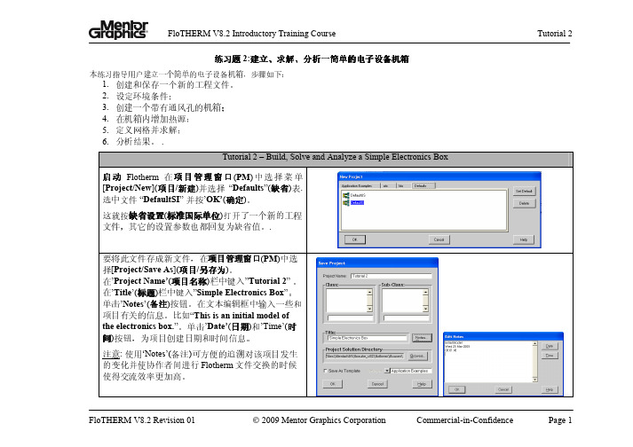
.Tutorial 2 – Build, Solve and Analyze a Simple Electronics Box启动Flotherm在项目管理窗口(PM)中选择菜单[Project/New](项目/新建)并选择“Defaults”(缺省)表.选中文件 “DefaultSI” 并按’OK’(确定)。
这就按缺省设置(标准国际单位)打开了一个新的工程文件,其它的设置参数也都回复为缺省值。
.要将此文件存成新文件,在项目管理窗口(PM)中选择[Project/Save As](项目/另存为)。
在’Project Name’(项目名称)栏中键入”Tutorial 2” 。
在’Title’(标题)栏中键入”Simple Electronics Box”。
单击’Notes’(备注)按钮。
在文本编辑框中输入一些和项目有关的信息。
比如“This is an initial model ofthe electronics box.”。
单击’Date’(日期)和’Time’(时间)按钮,为项目创建日期和时间信息。
注意: 使用‘Notes’(备注)可方便的追溯对该项目发生的变化并使协作者间进行Flotherm文件交换的时候使得交流效率更加高。
Tutorial 2 – Build, Solve and Analyze a Simple Electronics Box整体的缺省尺寸单位可在项目管理窗口(PM )中设置。
在菜单条上, 选择[Edit/Units ](编辑/单位)。
在 ‘Unit Class ’ (单位类型)下面选中 ‘LENGTH ’(长处) 并 在 ‘Use Units ’(使用单位) 中选择’ mm ’。


1. 引言随着电子设备向高集成度方向发展,系统的热功率密度越来越大,因此热设计技术在电子设备中显得越来越重要。
目前公司主要采用Flotherm商业热分析软件进行系统级、板级的热分析。
热分析过程主要分为建造模型、为模型添加物性、网格划分、求解与后处理几个过程。
在热分析的过程当中,准确的建造模型、添加物性固然重要,它将直接影响到结果的准确性,然而网格划分对于初学者来说也很重要,劣质的网格可能会导致求解发散,甚至会导致得到错误的结果。
所有的错误都会体现在残差曲线中,本文主要讲述各种有问题的残差曲线,并详细讲述处理的方法。
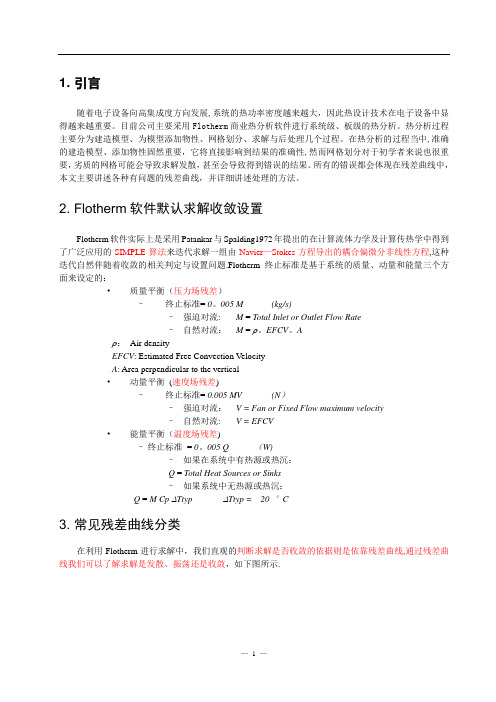
2. Flotherm软件默认求解收敛设置Flotherm软件实际上是采用Patankar与Spalding1972年提出的在计算流体力学及计算传热学中得到了广泛应用的SIMPLE算法来迭代求解一组由Navier—Stokes方程导出的耦合偏微分非线性方程,这种迭代自然伴随着收敛的相关判定与设置问题.Flotherm终止标准是基于系统的质量、动量和能量三个方面来设定的:•质量平衡(压力场残差)–终止标准= 0。
005M(kg/s)–强迫对流: M = Total Inlet or Outlet Flow Rate–自然对流:M = ρ。
EFCV。
Aρ:Air densityEFCV: Estimated Free Convection VelocityA: Area perpendicular to the vertical•动量平衡(速度场残差)–终止标准= 0.005MV(N)–强迫对流:V = Fan or Fixed Flow maximum velocity–自然对流: V = EFCV•能量平衡(温度场残差)–终止标准= 0。
005 Q (W)–如果在系统中有热源或热沉:Q = Total Heat Sources or Sinks–如果系统中无热源或热沉:Q = M Cp ∆Ttyp ∆Ttyp = 20 °C3. 常见残差曲线分类在利用Flotherm进行求解中,我们直观的判断求解是否收敛的依据则是依靠残差曲线,通过残差曲线我们可以了解求解是发散、振荡还是收敛,如下图所示.图一:残差曲线1) 对于大多数残差曲线收敛且监控点温度稳定的情况下,我们可以认为得到了稳定正确的数值 解,当然有时也会由于温度梯度较大的位置网格数量不足或者两种不同的物体划分到同一网格得到具有较大误差的结果。

Tutorial 2. Solid-Solid Heat ConductionIntroductionThis tutorial illustrates the setup and solution of a multi-domain problem. Distinct sets of equations are solved on non-overlapping subdomains. The problem involves a heat transfer calculation between two solids (heat conduction), with each solid having a different thermal conductivity.In this tutorial, you will learn how to:• Start POLYDATA from Workbench• Create a new task• Create multiple sub-tasks• Set material properties and boundary conditions for a solid-solid heat conduction problemPrerequisitesThis tutorial assumes that you are familiar with the menu structure in POLYDATA and Workbench, and that you have solved or read Tutorial 1. Some steps in the setup procedure will not be shown explicitly.Problem DescriptionThis tutorial examines the heat conduction in two solid square bodies, each of length 100 cm, as shown in Figure 2.1. A heat transfer calculation is performed between the solid bodies. To solve the fully coupled problem, we will define two sub-tasks, one each for solid 1 and solid 2. Each sub-task will contain a particular model, domain of definition, material properties, and boundary conditions, including interface conditions with the other sub-task.The two heat conduction problems are coupled because the global solution of the problem depends on the values of the solution variables at the intersection of the solid domains. The two subdomains are shown in Figure 2.2.Solid-Solid heat ConductionThe partial differential equation solved in both subdomains corresponds to the steady state heat conduction model:Figure 2.1: Schematic Diagram of the Solid Square BodiesFigure 2.2: Boundaries and Subdomains for the Solid-Solid Heat Conduction Problem()0T∇Tk(2.1))⋅(=∇where T∇ is the temperature gradient and k(T) is the thermal conductivity. solid 1 and solid 2 have thermal conductivity (k) of 10 W/m.°C and 35 W/m.°C, respectively.Solid-Solid heat Conduction The boundary sets for the problem are shown in Figure 2.2, and the conditions at the boundaries of the domains are as follows:• boundary 1: insulated• boundary 2: T = 100°C• boundary 3: insulated• boundary 4: T = 150°CAn interface is defined at the intersection of subdomain 1 and subdomain 2. Preparation1. Copy the file, heatcond/heatcond.msh from the POLYFLOW documentation CD or installation area to your working directory (as described in Tutorial 1).2. Start Workbench from startÆAll ProgramsÆAnsys13.0ÆWorkbench.Step 1: Project and Mesh1. Create a Polyflow Analysis system by drag and drop in workbench, import the mesh file (heatcond.msh), and double-click the Setup cell of the analysis to start POLYDATA.For detailed information on how to do this, refer to Tutorial 1.When POLYDATA starts, the Create a new task menu item is highlighted, and the geometry for the problem is displayed in the Graphics Display window.Step 2: Models, Material Data, and Boundary ConditionsIn this step, define a new task representing the solid-solid heat conduction problem. Since this example is focused on the heat transfer calculation between two solids with different thermal conductivities, the heat conduction problem for the solids is described in two different sub-tasks. However, the task attributes are the same for both the sub-tasks, so define a single task for the coupled problem.1. Create a task for the model.Create a new taskSolid-Solid heat Conduction(a) Retain the following (default) options:• F.E.M. task• Steady-state problem• 2D planar geometryAs seen in the Graphics Display window, this problem is geometrically defined ina 2D Cartesian reference frame (x,y). Hence, choose 2D planar geometry.A Steady-state condition is assumed for the problem.SelectAccept the current setup.(b)The Create a sub-task menu item is highlighted.At this point (i.e., when Create a sub-task is highlighted), if you realize that you have made a mistake in creating the task, you can return to the previous menu by doing the following:1. Select Upper level menu to return to the top-level POLYDATA menu.2. Select Redefine global parameters of a task and make the necessary changes.3. Select Accept the current setup when you are satisfied with the corrected settings.4. Select F.E.M. Task 1. The Create a sub-task menu item is highlighted.Step 2a: Definition of Sub-Task 1In this step, define the heat conduction problem, identify the domain of definition, set the relevant material properties for solid 1, and define boundary conditions along its boundaries.1. Create a sub-task for solid 1.Create a sub-taskHeat conduction problem.(a)SelectA panel appears, asking for the title of the problem.Solid-Solid heat ConductionEntersolid 1 as the New value and click OK.(b)The Domain of the sub-task menu item is highlighted.At this point (i.e., when Domain of the sub-task is highlighted), if you realize that you have made a mistake in creating the sub-task, you can return to the previous menu by doing the following:1. Select Upper level menu.2. Select Redefine global parameters of a sub-task and make the necessary changes.3. Select Upper level menu.4. Select solid 1 at the bottom of the existing menu.The Domain of the sub-task menu item is highlighted.2. Define the domain where the sub-task applies (subdomain 1).There are two subdomains in this problem. Each sub-task is defined with its own model, material properties, and boundary conditions. To solve the coupled problem, the domain is divided into two subdomains with a common intersection and a subtask is defined on each of the non-overlapping subdomains. Sub-task 1 is defined for subdomain 1, since subdomain 1 represents solid 1 (as shown in Figure 2.2).Domain of the sub-task(a) Select Subdomain 2 and click Remove.Solid-Solid heat Conduction(b) Click on Upper level menu at the top of the panel.The Material data menu item is highlighted.3. Specify the material properties for solid 1.POLYDATA indicates which material properties are relevant for your sub-task by graying out the irrelevant properties. For this model, define only the constant thermal conductivity (k) of the material.Material data(a) Select Thermal conductivity.As shown at the top of the menu, the thermal conductivity is defined as a non-linear function of temperature:k = a + bt + ct2 + dt3 (2.2)Solid-Solid heat Conduction In this problem, thermal conductivity is assumed to be a constant, so only the constant coefficient ‘a’ is modified.Modify a(b) Enter 10 as the New value and click OK.(c) Check if the value of the thermal conductivity is correct, and repeat theprevious steps if you need to modify it again.(d) Select Upper level menu two times to leave the material data specification.The Thermal boundary conditions menu item is highlighted.4. Specify the boundary conditions for subdomain 1.In this step, set the conditions at each of the boundaries of the domain. When a boundary set is selected, it is highlighted in red in the graphics window.Thermal boundary conditionsSolid-Solid heat Conduction(a) Set the conditions along the intersection of subdomain 1 and subdomain 2.Set an interface condition at the intersection of subdomain 1 and subdomain 2. This condition ensures the continuity of the temperature field and the heat flux along the interface. Since the problem is a coupled one, the condition of continuity is essential for the global solution of the temperature and heat flux variables.imposedalong subdomain 2 and click Modify.TemperatureSelecti.Interface.ii.SelectFor an interface condition, both the heat flux and the temperature areusually continuous along the interface. It is possible to specify a non-zerovalue for the heat flux jump (dq), but this is mainly used in problemswhere internal radiation is simulated. Here, accept the default value forthe definition of heat flux discontinuity, i.e., dq=0.iii. Select Upper level menu to accept the default option.Solid-Solid heat Conduction(b) Set the conditions at boundary 1.Impose a zero conductive heat flux along this boundary.imposed along boundary 1 and click Modify.Temperaturei.Selectii. Select Insulated boundary / symmetry.(c) Set the conditions at boundary 4.Impose a constant value for the temperature along this boundary.Temperatureimposed along boundary 4 and click Modify.Selecti.imposed.Temperatureii.SelectConstant.Selectiii.A panel appears, asking for the value of the constant temperature.iv. Enter 150 as the New value and click OK.v. Select Upper level menu.(d) Click on Upper level menu at the top of the Thermal boundary conditions panel.(e) Select Upper level menu at the top of the solid 1 sub-task menu.Step 2b: Definition of Sub-Task 2Solid-Solid heat ConductionIn this step, define the heat conduction problem, identify the domain of definition, set the relevant material properties for solid 2, and define boundary conditions along its boundaries.1. Create a sub-task for solid2.Create a sub-task(a) POLYDATA asks whether you want to copy data from an existing sub-task.(b) Click No, since this sub-task will have different parameters associated with it.(c) Select Heat conduction problem.A panel appears, asking for the title of the problem.i. Enter solid 2 as the New value and click OK.2. Define the domain where the sub-task applies (subdomain 2).Domain of the sub-task(a) Select Subdomain 1 and click Remove.(b) Click on Upper level menu at the top of the panel.The Material data menu item is highlighted.3. Specify the material properties for solid 2.Material dataIn this problem, specify a constant value for the thermal conductivity (k).(a) Select Thermal conductivity.In this problem, thermal conductivity is assumed to be a constant, so only the constant coefficient a is modified.Modifya(b) Enter 35 as the New value and click OK.(c) Check whether the value of the thermal conductivity is correct and repeat theprevious steps if you need to modify it again.(d) Select Upper level menu two times to leave the material data specification.The Thermal boundary conditions menu item is highlighted.4. Specify the boundary conditions for subdomain 2.In this step, set the conditions at each of the boundaries of the domain. When a boundary set is selected, it is highlighted in red in the graphics window.Thermal boundary conditions(a) Set the conditions at the intersection of subdomain 1 and subdomain 2.Set an interface condition at the intersection of the subdomains.imposedalong subdomain 1 and click Modify.TemperatureSelecti.Interface.Selectii.iii. Select Upper level menu to accept the default option for continuity offlux.temperatureandheat(b) Set the conditions at boundary 1.Impose a zero conductive heat flux along this boundary.imposed along boundary 1 and click Modify.SelectTemperaturei.ii. Select Insulated boundary / symmetry.(c) Set the conditions at boundary 2.Impose a constant value for the temperature along this boundary.imposed along boundary 2 and click Modify.TemperatureSelecti.imposed.TemperatureSelectii.SelectConstant.iii.A panel appears, asking for the value of the constant temperature.iv. Enter 100 as the New value and click OK.v. Select Upper level menu.(d) Set the conditions at boundary 3.Impose a zero conductive heat flux along this boundary.imposed along boundary 3 and click Modify.TemperatureSelecti.ii. Select Insulated boundary / symmetry.(e) Click on Upper level menu at the top of the Thermal boundary conditions panel.(f) Select Upper level menu two times to return to the top-level POLYDATA menu.Step 3: Save the Data and Exit POLYDATAAfter defining your model in POLYDATA, save the data file. In the next step, you will read this data file into POLYFLOW and calculate a solution.Save and exitPOLYDATA asks you to confirm the current system units and fields that are to be saved to the results file for post-processing.1. Select Upper level menuThis confirms that the default units are correct.2. Select Accept.This confirms that the default Current field(s) are correct.3. Select Continue.This accepts the default names for the graphical output files (cfx.res) that are to be saved for post-processing, and the POLYFLOW format results file (res).Step 4: SolutionIn this step, run POLYFLOW to calculate a solution for the model you just defined using POLYDATA.1. Run POLYFLOW by righ click on Solution cell of the simulation and click on Update button.This command executes POLYFLOW using the data file as standard input, and writes information about the problem description, calculations, and convergence to a listing file.2. Check for convergence in the listing file.Right click on Solution cell and click on Listing Viewer…Workbench opens View listing file panel, which displays the listing file.Step 5: Post-processingUse CFD-Post to view the results of the POLYFLOW simulation.1. Double click on Results cell in the workbench analysis and read the results files saved by POLYFLOW.CFD-Post reads the mesh information and the solution fields that were saved to the results file.2. Align the viewIn the graphical window, right-click, and select the option “Predefined Camera”(a) Select “View Towards –z”.The central-mouse button allows you to zoom in and zoom out.The left-mouse button allows to rotate the image.The right-mouse button allows you to translate the image.3. Display contours of temperature.Since the coupled problem analyzes the heat transport in solids, display contours of the temperature field to view the heat transfer between the solids.(a) Select the domain.→Unroll Mesh regionsOutlinetabi. under Mesh Regions, select SD_1 Hex and SD_2 Hex.(b) Select the variable and display the results.ii. In the graphic window, right-click on the left-hand subdomainiii. Under “Colour”, select the field “TEMPERATURE”.iv. Repeat the above operations ii and iii for the right-hand subdomain.Figure 2.3: Contours of Static TemperatureIn Figure 2.3, the temperature varies from the imposed value of 100 on the right-hand side of solid 2, to 150 on the left-hand side of solid 1. Also, the temperature isolines are perpendicular to the walls where the heat flux was set to zero (boundaries 1 and 3); a zero heat flux implies that the temperature gradient along a normal to the wall is zero. 4. Temperature profile along a horizontal line.Plot the temperature profile along a horizontal line in the middle of the domain. For this, we first create a line and subsequently ask a plot on that line.i. Under “Location”, select “Line”, enter a name.ii. Define the line by two points (0,50,0) and (200,50,0).“Apply”.iii.onClickiv. Click on the Chart button , enter a name, and click on OK.v. In the Details of chart, select the tab “Chart Line 1”vi. Select the location: the line defined above.vii. Select X along the X-axis and TEMPERATURE along the Y-axis.viii. Under the tab “Chart”, modify the title, if needed.Apply.ix.ClickonFigure 2.4: Temperature Along the Line y = 50In Figure 2.4, the slope of the curve for subdomain 1 is different from that forsubdomain 2. The slope of the curve corresponds to the temperature gradient.The gradient is smaller in subdomain 2 because solid 2 has a higher heatconductivity, i.e., the heat is more easily conducted in solid 2 than in solid 1. Aneven higher conductivity in solid 2 would lead to a flatter temperature curve forsolid 2.SummaryThis tutorial introduced the concept of a multi-domain calculation, where two distinct sets of equations were solved on non-overlapping subdomains. The creation of a single task for solving two coupled heat conduction problems has been demonstrated. Each heat conduction problem was defined in a sub-task, and then the two sub-tasks were solvedsimultaneously in the same task.。
教程4—利用FLOMCAD进行CAD几何模型导入该教程希望通过练习以下一些操作加深对FLOMCAD的理解:1. 导入一个在CAD工具里建立的2U的机箱(名为2U pizza box)。
2. 简化该模型,去除与EMC分析意义无关的部分3. 把几何模型转换为FLOEMC实体4. 将几何模型导入FLOEMC5. 在FLOEMC中检查确认导入的模型是否正确I"訓dUbl 他Us/rinjEzIwUij UnM教程4—利用FLOMCAD CAD几何模型导入从开始菜单[Start/Programs/Flomerics/FLOEMC 6.1/FLOEMC6.1]启动FLOEMC,或直接用桌面快捷方式窗口弹出,任务管理器P roject Ma nager (PM)即打开。
点击FLOMCAD快捷键同时打开,关闭Message窗口。
注意:也可以[Start/Programs/Flomerics/FLOEMC,FLOMCAD 和Message窗口会I IH I*舅ffl lUHJBTlCTT r- 2f .'Piceci 立)如fenriMF i曲加5A 垂^* Ffe^= H种站■H EU爭时v rfe /金亍芒并壬]唱-;:,O H r tdw以HQ I SvJan■ ft^gl^yp^bk令I" 11CifrV話易■rtwaiE Jl P pi教程4—利用FLOMCAD进行CAD几何模型导入FLOMCAD 启动后,操作External/lmport SAT,找到并打开Open 2UP izzaBox.SAT由于可能会报告出错信息,因此在模型简化过程中不要关闭窗口。
3DTipr-^TEPII .'I.I 鈕*t -V5'All||_&0&f.SAT* ]UJXM=*n^e« JA7Atii-Tfdiiiy S4TAhijti.5*T ^Apc-satA啊.皿ArilonriewMt在打开模型过程中会弹出MCAD Monitor Window的窗口,观察窗口中的信息,可以看到FLOMCAD正在转换已经在CAD 工具中命名过了的模型部件。