Hyper-Nastran接口视频教程之模态分析与瞬态分析
- 格式:pdf
- 大小:328.20 KB
- 文档页数:34
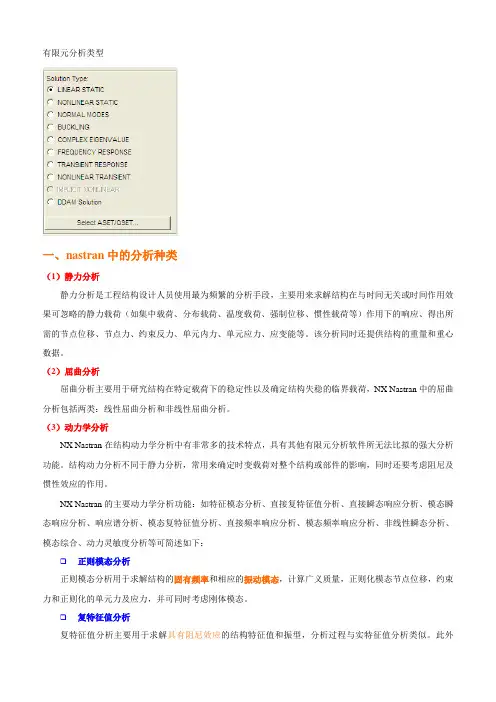
有限元分析类型一、nastran中的分析种类(1)静力分析静力分析是工程结构设计人员使用最为频繁的分析手段,主要用来求解结构在与时间无关或时间作用效果可忽略的静力载荷(如集中载荷、分布载荷、温度载荷、强制位移、惯性载荷等)作用下的响应、得出所需的节点位移、节点力、约束反力、单元内力、单元应力、应变能等。
该分析同时还提供结构的重量和重心数据。
(2)屈曲分析屈曲分析主要用于研究结构在特定载荷下的稳定性以及确定结构失稳的临界载荷,NX Nastran中的屈曲分析包括两类:线性屈曲分析和非线性屈曲分析。
(3)动力学分析NX Nastran在结构动力学分析中有非常多的技术特点,具有其他有限元分析软件所无法比拟的强大分析功能。
结构动力分析不同于静力分析,常用来确定时变载荷对整个结构或部件的影响,同时还要考虑阻尼及惯性效应的作用。
NX Nastran的主要动力学分析功能:如特征模态分析、直接复特征值分析、直接瞬态响应分析、模态瞬态响应分析、响应谱分析、模态复特征值分析、直接频率响应分析、模态频率响应分析、非线性瞬态分析、模态综合、动力灵敏度分析等可简述如下:❑正则模态分析正则模态分析用于求解结构的固有频率和相应的振动模态,计算广义质量,正则化模态节点位移,约束力和正则化的单元力及应力,并可同时考虑刚体模态。
❑复特征值分析复特征值分析主要用于求解具有阻尼效应的结构特征值和振型,分析过程与实特征值分析类似。
此外Nastran的复特征值计算还可考虑阻尼、质量及刚度矩阵的非对称性。
❑瞬态响应分析(时间-历程分析)瞬态响应分析在时域内计算结构在随时间变化的载荷作用下的动力响应,分为直接瞬态响应分析和模态瞬态响应分析。
两种方法均可考虑刚体位移作用。
直接瞬态响应分析该分析给出一个结构随时间变化的载荷的响应。
结构可以同时具有粘性阻尼和结构阻尼。
该分析在节点自由度上直接形成耦合的微分方程并对这些方程进行数值积分,直接瞬态响应分析求出随时间变化的位移、速度、加速度和约束力以及单元应力。
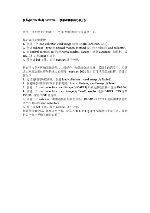
从hypermesh到nastran——模态和瞬态动力学分析鼓捣了几天终于行的通了,把自己的经验给大家分享一下。
模态分析关键步骤:1. 创建一个load collector, card image选择EIGRL(LANCZOS方法)。
2. 创建subcase,type为normal modes, method选中刚才创建的load collector。
3. 在control cards的sol选择nomal modes,param中选择autospec, 如果想生成op2文件,把post也选上4. 导出成bdf文件,启动nastran进行分析。
瞬态动力学分析如果激励是力比较好作,如果是强迫位移,老版本的需要用大质量或大刚度法把位移转换成力的载荷。
nastran 2001版以后可以直接加位移,关键步骤如下:1. 定义随时间历程曲线,创建load collectors,card image为Tabled12. 创建瞬态相应的时间步长和时间,load collectors, card image为Tstep3. 创建一个load collectors,card image为DAREA(如果是强迫位移不能用DAREA)4. 创建一个load collectors,card image为Tload1, excited选择DAREA,TID选择TSTEP,注意TYPE的选择。
5. 创建一个subcase,类型选择直接瞬态分析,DLOAD和TSTEP选择刚才创建的两个相对应的load collectors6. 导出成bdf文件,提交nastran进行分析。
如果是强迫位移,还要多两个卡,就是SPCD, LSEQ详细步骤跟以上差不多,只要把各个卡片弄懂了就很容易了。
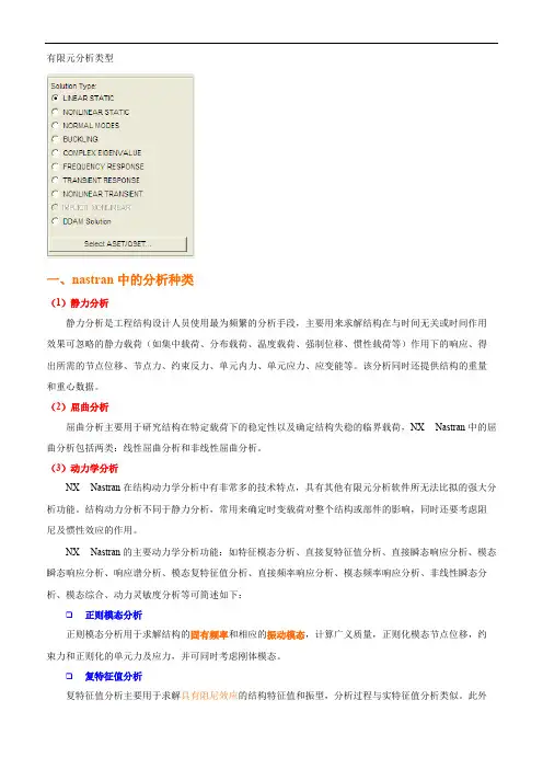
有限元分析类型一、nastran中的分析种类(1)静力分析静力分析是工程结构设计人员使用最为频繁的分析手段,主要用来求解结构在与时间无关或时间作用效果可忽略的静力载荷(如集中载荷、分布载荷、温度载荷、强制位移、惯性载荷等)作用下的响应、得出所需的节点位移、节点力、约束反力、单元内力、单元应力、应变能等。
该分析同时还提供结构的重量和重心数据。
(2)屈曲分析屈曲分析主要用于研究结构在特定载荷下的稳定性以及确定结构失稳的临界载荷,NX Nastran中的屈曲分析包括两类:线性屈曲分析和非线性屈曲分析。
(3)动力学分析NX Nastran在结构动力学分析中有非常多的技术特点,具有其他有限元分析软件所无法比拟的强大分析功能。
结构动力分析不同于静力分析,常用来确定时变载荷对整个结构或部件的影响,同时还要考虑阻尼及惯性效应的作用。
NX Nastran的主要动力学分析功能:如特征模态分析、直接复特征值分析、直接瞬态响应分析、模态瞬态响应分析、响应谱分析、模态复特征值分析、直接频率响应分析、模态频率响应分析、非线性瞬态分析、模态综合、动力灵敏度分析等可简述如下:❑正则模态分析正则模态分析用于求解结构的固有频率和相应的振动模态,计算广义质量,正则化模态节点位移,约束力和正则化的单元力及应力,并可同时考虑刚体模态。
❑复特征值分析复特征值分析主要用于求解具有阻尼效应的结构特征值和振型,分析过程与实特征值分析类似。
此外Nastran的复特征值计算还可考虑阻尼、质量及刚度矩阵的非对称性。
❑瞬态响应分析(时间-历程分析)瞬态响应分析在时域内计算结构在随时间变化的载荷作用下的动力响应,分为直接瞬态响应分析和模态瞬态响应分析。
两种方法均可考虑刚体位移作用。
直接瞬态响应分析该分析给出一个结构随时间变化的载荷的响应。
结构可以同时具有粘性阻尼和结构阻尼。
该分析在节点自由度上直接形成耦合的微分方程并对这些方程进行数值积分,直接瞬态响应分析求出随时间变化的位移、速度、加速度和约束力以及单元应力。
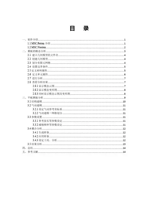
目录一、软件介绍 (1)1.1 MSC.Patran介绍 (1)1.2 MSC.Nastran (2)二、翼板的模态分析 (3)2.1 建立几何模型的文件名 (4)2.2 创建几何模型 (4)2.3 划分有限元网格 (4)2.4 设置边界条件 (5)2.5定义材料属性 (5)2.6 定义单元属性 (6)2.7 进行分析 (7)2.8 查看分析结果 (7)2.8.1显示模态云图 (7)2.8.2显示模态变形图 (8)2.8.3同时显示模态云图及变形图 (8)三、平板颤振分析 (9)3.1结构建模 (10)3.2气动建模 (11)3.2.1设定气动参考坐标系 (11)3.2.2气动建模-网格划分 (11)3.3参数设置 (11)3.3.1参考弦长等参数设定 (11)3.3.2减缩频率等参数设定 (11)3.4耦合分析 (12)3.4.1生成样条 (12)3.4.2应用样条 (12)3.4.3设定工况、分析 (12)3.5结果分析 (13)四、总结 (14)五、参考文献 (14)一、软件介绍1.1 MSC.Patran介绍MSC.Patran(后称Patran)是一个集成的并行框架式有限元前后处理及分析仿真系统。
Patran最早由美国宇航局(NASA)倡导开发, 是工业领域最著名的并行框架式有限元前后处理及分析系统, 其开放式、多功能的体系结构可将工程设计、工程分析、结果评估、用户化设计和交互图形界面集于一身, 构成一个完整的CAE集成环境。
使用Patran, 可以帮助产品开发用户实现从设计到制造全过程的产品性能仿真。
Patran拥有良好的用户界面, 既容易使用又方便记忆。
Patran作为一个优秀的前后处理器, 具有高度的集成能力和良好的适用性, 具体表现在:1.模型处理智能化。
为了节约宝贵的时间, 减少重复建模, 消除由此带来的不必要的错误, Patran应用直接几何访问技术(DGA), 能够使用户直接从一些世界先导的CAD/CAM系统中获取几何模型, 甚至参数和特征。

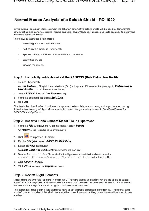
Normal Modes Analysis of a Splash Shield - RD-1020In this tutorial, an existing finite element model of an automotive splash shield will be used to demonstrate how to set up and perform a normal modes analysis. HyperMesh post-processing tools are used to determine mode shapes of the model.The following exercises are included:•Retrieving the RADIOSS input file•Setting up the model in HyperMesh•Applying Loads and Boundary Conditions to the Model•Submitting the job•Viewing the resultsStep 1: Launch HyperMesh and set the RADIOSS (Bulk Data) User Profileunch HyperMesh.A User Profiles… Graphic User Interface (GUI) will appear. If it does not appear, go to Preferences►User Profiles … from the menu on the top.2.Select RADIOSS in the User Profile dialog.3.From the extended list, select Bulk Data.4.Click OK.This loads the User Profile. It includes the appropriate template, macro menu, and import reader, paring down the functionality of HyperMesh to what is relevant for generating models in Bulk Data Format for RADIOSS and OptiStruct.Step 2: Import a Finite Element Model File in HyperMesh1.From the File pull-down menu on the toolbar, select Import….An Import… tab is added to your tab menu.2.Click to import an FE model.3.For the File type:, select RADIOSS (Bulk Data).4.Select the Files icon button.A Select RADIOSS (Bulk Data) file browser will pop up.5.Browse for sshield.fem file located in the HyperWorks installation directory under<install_directory>/tutorials/hwsolvers/radioss/ and select the file.6.Click Open►Import.7.Click Close to close the Import tab menu.Step 3: Review Rigid ElementsNotice there are two rigid "spiders" in the model. They are placed at locations where the shield is bolted down. This is a simplified representation of the interaction between the bolts and the shield. It is assumed that the bolts are significantly more rigid in comparison to the shield.The dependent nodes of the rigid elements have all six degrees of freedom constrained. Therefore, each "spider" connects nodes of the shell mesh together in such a way that they do not move with respect to one another.The following steps show how to review the properties of the rigid elements.1.From the 1D page, select the rigids.2.Click review.3.Select one of the rigid elements in the graphics region.In the graphics window, HyperMesh displays the IDs of the rigid element and the two end nodes and indicates the independent node with an 'I' and the dependent node with a 'D'. HyperMesh also indicates the constrained degrees of freedom for the selected element, through the dof checkboxes in the rigids panel. All rigid elements in this model should have all dofs constrained.4.Click return to go to the main menu.Step 4: Setting up the Material and Geometric PropertiesThe imported model has three component collectors with no materials. A material collector needs to be created and assigned to the shell component collectors. The rigid elements do not need to be assigned a material. Shell thickness values also need to be corrected.1.Select the Material Collectors toolbar button .2.Select the create subpanel using the radio buttons on the left-hand side of the panel.3.Click mat name = and enter steel.4.Select the desired color for the material steel by clicking on .5.Click card image = and select MAT1 from the pop-up menu.6.Click create/edit.The MAT1 card image pops up.7.For E, enter the value 2.0E5.8.For NU, enter the value 0.3.9.For RHO, enter the value 7.85E-9.If a quantity in brackets does not have a value below it, it is off. To change this, click the quantity in brackets and an entry field will appear below it. Click in the entry field, and a value can be entered.10.Click return.A new material, steel, has now been created. The material uses RADIOSS linear isotropic materialmodel, MAT1. This material has a Young's Modulus of 2E+05, a Poisson's Ratio of 0.3 and a material density of 7.85E-09. A material density is required for the normal modes solution sequence.At any time the card image for this collector can be modified using Card Editor.11.Click return to exit the Material Create panel.12.Select the Card Editor toolbar button .13.Click the down arrow on the right of the entity shown in the yellow box, select props from the extendedentity list.14.Click the yellow props button and then check the box next to design and nondesign.15.Click select.16.Make sure card image=is set to PSHELL.17.Click edit.The PSHELL card image for the design component collector pops up.18.Replace 0.300 in the T field with 0.25.19.Click return to save the changes to the card image.20.Click return to go to the main menu.Applying Loads and Boundary Conditions to the Model (Steps 5 - 7)The model is to be constrained using SPCs at the bolt locations, as shown in the following figure. The constraints will be organized into the load collector 'constraints'.To perform a normal modes analysis, a real eigenvalue extraction (EIGRL) card needs to be referenced in the subcase. The real eigenvalue extraction card is defined in HyperMesh as a load collector with an EIGRL card image. This load collector should not contain any other loads.Step 5: Create EIGRL card (to request the number of modes)If a quantity in brackets does not have a value below it, it is off. To change this, click on the quantity in brackets and an entry field will appear below it. Click on the entry field, and a value can be entered.Step 6: Create Constraints at Bolt LocationsSelecting nodes for constraining the bolt locations 1.Click the Load Collectors toolbar button .2.Select the create subpanel, using the radio buttons on the left-hand side of the panel.3.Click loadcol name = and enter EIGRL .4.Click card image= and select EIGRL from the pop-up menu.5.Click create/edit .6.For V2, enter the value 200.000.7.For ND , enter the value 6.8.Click return to save changes to the card image.1.Click loadcol name = and enter constraints .2.Click the switch next to card image and select no card image .3.Click create > return .4.From Analysis page, click the constraints panel and make sure that the createsubpanel is active.5.Select the two nodes, shown in the figure above, at the center of the rigid spiders, by clicking on them in the graphics window.6.Constrain all dofs with a value of 0.0.7.Click Load Type= and select SPC .8.Click createTwo constraints are created. Constraint symbols (triangles) appear in the graphics window at theselected nodes. The number 123456 is written beside the constraint symbol, if the label constraints is checked ‘ON’, indicating that all dofs are constrained.9.Click return to go the main menu.Step 7: Create a Load Step to perform Normal Modes Analysis1.From the Analysis page, enter the loadsteps panel.2.Click name = and enter bolted.3.Click the type: switch and select normal modes from the pop-up menu.4.Check the box preceding SPC.An entry field appears to the right of SPC.5.Click on the entry field and select constraints from the list of load collectors.6.Check the box preceding METHOD(STRUCT).An entry field appears to the right of METHOD.7.Click on the entry field and select EIGRL from the list of load collectors.8.Click create.A RADIOSS subcase has been created which references the constraints in the load collector constraintsand the real eigenvalue extraction data in the load collector EIGRL.9.Click return to go to the main menu.Submitting the JobStep 8: Running Normal Modes Analysis1.From the Analysis page, enter the RADIOSS panel.2.Click save as… following the input file:field.A Save file… browser window pops up.3.Select the directory where you would like to write the file and, in File name:, entersshield_complete.fem.4.Click Save.Note that the name and location of the sshield_complete.fem file shows in the input file: field.5.Set the export options:toggle to all.6.Click the run options: switch and select analysis.7.Set the memory options: toggle to memory default.8.Click Radioss.This launches the RADIOSS job.If the job was successful, new results files can be seen in the directory where the RADIOSS model file was written. The sshield_complete.out file is a good place to look for error messages that will help to debug the input deck if any errors are present.The default files written to your directory are:sshield_complete.html HTML report of the analysis, giving a summary of the problemformulation and the analysis results.sshield_complete.out RADIOSS output file containing specific information on the file setup, the set up of your optimization problem, estimates for the amountof RAM and disk space required for the run, information for eachoptimization iteration, and compute time information. Review this fileReview the Results using HyperViewEigenvector results are output by default, from RADIOSS for a normal modes analysis. This section describes how to view the results in HyperView.Step 9: Load the Model and Result Files into the Animation WindowIn this section, you will load a HyperView .h3d file into the HyperView animation window.HyperView is launched and the sshield_complete.h3d file is loaded.Step 10: View Eigen VectorsIt is helpful to view the deformed shape of a model to determine if the boundary conditions have been defined correctly and also to check if the model is deforming as expected. In this section, use the Deformed panel to review the deformed shape for last Mode .This means that the maximum displacement will be 10 modal units and all other displacements will be proportional.Using a scale factor higher than 1.0 amplifies the deformations while a scale factor smaller than 1.0 would reduce them. In this case, we are accentuating displacements in all directions.A deformed plot of the model overlaid on the original undeformed mesh is displayed in the graphics window. for warnings and errors.sshield_complete.h3dHyper 3D binary results file. sshield_complete.stat Summary of analysis process, providing CPU information for eachstep during analysis process. 1.Click the HyperView button in the RADIOSS panel. 2.Click Close to exit the Message Log menu that appears.1.Click on the switch next to the traffic light signaland select Modal .2.Select the Deformed toolbar button.3.Leave Result type:set to Eigen Mode (v).4.Set Scale: to Model units .5.Set Type: to Uniform and enter in a scale factor of 10 for Value:.6.Click Apply .7.Under Undeformed shape:, set Show: to Wireframe .8.From the Graphics pull-down menu, select Select Load Case to activate the Load Case andSimulation Selection dialog, as shown below.Step 11: A few points to be notedIn this analysis, it was assumed that the bolts were significantly stiffer than the shield. If the bolts needed to be made of aluminum and the shield was still made of steel, would the model need to be modified, and the analysis run again?It is necessary to push the natural frequencies of the splash shield above 50 Hz. With the current model, there should be one mode that violates this constraint: Mode 1. Design specifications allow the innerdisjointed circular rib to be modified such that no significant mass is added to the part. Is there a configuration for this rib within the above stated constraints that will push the first mode above 50 Hz? See tutorial OS-2020 to optimize rib locations for this part.Go ToRADIOSS, MotionSolve, and OptiStruct Tutorials9.Select Mode 6 - F=1.496557E+02 from the list and click OK to view Mode 6.10.To animate the mode shape, click the animation mode: modal.11.To control the animation speed, use the Animation Controls accessed with the director’s chair toolbar button .12.You could also review the rest of the mode shapes.。
基于HyperMesh与Nastran联合仿真引言随着科技的进步和工程领域的发展,仿真技术在工程设计和分析中扮演着越来越重要的角色。
HyperMesh和Nastran是两个在工程仿真中广泛应用的软件工具,它们的联合使用可以实现更精确和可靠的仿真结果。
本文将介绍基于HyperMesh与Nastran联合仿真的基本原理和使用方法,并通过案例分析来展示其在工程实践中的应用。
一、HyperMesh简介HyperMesh是由美国公司Altair Engineering开发的一款高性能有限元预处理软件。
它提供了一个功能强大而简洁的界面,能够帮助工程师快速准确地构建计算模型。
HyperMesh支持多种CAD格式的导入,并提供了丰富的网格划分和修改工具。
此外,HyperMesh还包含了一系列的仿真后处理功能,可以帮助用户对仿真结果进行可视化和分析。
二、Nastran简介Nastran是由美国公司NASA开发的一款经典的有限元分析软件。
它是目前工程仿真领域最常用的软件之一,可以广泛应用于结构、振动、热传导和流体力学等领域。
Nastran采用了成熟稳定的数值方法和高效快速的求解算法,能够准确地预测结构的运行和响应。
Nastran提供了一个强大的命令行界面,可以通过输入Nastran语句进行仿真模型的定义、材料属性的指定和边界条件的设置等。
三、HyperMesh与Nastran联合仿真原理HyperMesh与Nastran联合仿真的基本原理是将HyperMesh生成的几何模型转化为Nastran所需的有限元网格模型,并将该模型输入到Nastran求解器中进行仿真分析。
具体包括以下几个步骤:1.导入模型:将CAD模型导入HyperMesh中,并进行必要的几何处理和修正。
2.网格划分:使用HyperMesh提供的网格划分工具对模型进行网格划分,生成满足仿真要求的有限元网格。
3.材料属性和边界条件设置:通过HyperMesh进行材料属性的指定和边界条件的设置。
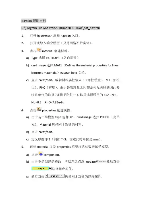
Nastran帮助文档D:\Program Files\nastran2010\md20101\Doc\pdf_nastran1、打开hypermesh选择nastran入口。
2、打开或导入响应模型(只是网格不带实体)。
3、点击material创建材料。
a)Type选择ISOTROPIC(各向同性)b)card image选择MAT1(Defines the material properties for linearisotropic materials.)nastran help文档。
c)点击creat/edit,编辑材料属性输入E(弹性模量)、NU(泊松比)、RHO(密度)。
由于各物理量之间都是相互关联的因此要注意单位的选择(详情见附件一)。
这里选择通用的E=2.07e5,NU=0.3,RHO=7.83e-9。
4、点击properties创建属性。
a)由于是二维模型type选择2D。
Card image选择PSHELL(壳单元)。
Material选择刚才新建的材料。
b)点击creat/edit。
c)定义厚度即T(例如T=3,注意此时单位是mm)。
5、创建material以及properties后要将这些数据赋予模型。
a)点击component。
b)由于不是创建是修改,所以左边点选update然后双击选择相应部件。
c)然后双击选择刚才新建的厚度属性。
d)最后点击update。
6、创建加载情况,点击。
a)加一个单位动态激励。
创建名为excite的激励,点击creat。
b)加载单位激励。
Analysis-constraints 确定加载力的方向。
例如X正方向加载激励,只需要勾选dof1,且值为1。
Load types选择DAREA。
然后在模型上选择一点,最后点击create。
c)创建激励频率范围。
创建名为tabled1,card image为TABLED1,点击creat/edit。
设置TABLED1_NUM=2,x(1)=0,y(1)=1,x(2)=1000,y(2)=1.d)创建rload2目的连接excite和tabled1.card image选择RLOAD2,点击creat/edit。
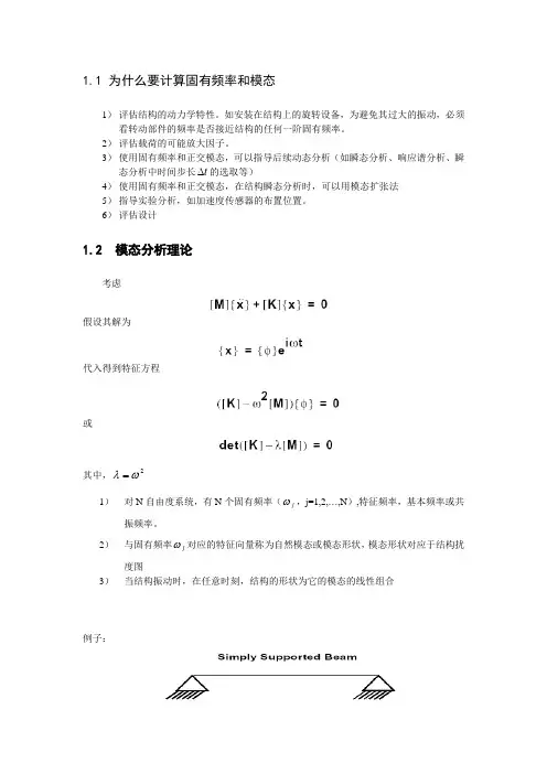
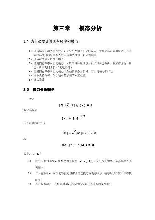
1.1 为什么要计算固有频率和模态1) 评估结构的动力学特性。
如安装在结构上的旋转设备,为避免其过大的振动,必须看转动部件的频率是否接近结构的任何一阶固有频率。
2) 评估载荷的可能放大因子。
3) 使用固有频率和正交模态,可以指导后续动态分析(如瞬态分析、响应谱分析、瞬态分析中时间步长t ∆的选取等)4) 使用固有频率和正交模态,在结构瞬态分析时,可以用模态扩张法 5) 指导实验分析,如加速度传感器的布置位置。
6) 评估设计1.2 模态分析理论考虑假设其解为代入得到特征方程或其中,2ωλ=1) 对N 自由度系统,有N 个固有频率(j ω,j=1,2,…,N ),特征频率,基本频率或共振频率。
2) 与固有频率j ω对应的特征向量称为自然模态或模态形状,模态形状对应于结构扰度图3) 当结构振动时,在任意时刻,结构的形状为它的模态的线性组合例子:1.3 自然模态与固有频率性质(1)正交性ω的单位(2)jω单位为rad/s, 也可以表示为Hz (cycles/seconds),二者换算关系为j(3)刚体模态图为一未约束结构,有刚体模态如果结构完全未约束,有刚体模态存在(应力-自由模态)或机构运动,至少有一固有频率为0。
(4)自然模态的倍数依然为自然模态如:代表相同的振动模态(5)模态的标准化1.4 模态能量(1)应变-位移关系(2)应力-应变关系(3)静力-位移关系(4)单元应变能因此,对给定的模态位移模态应变为模态应力为模态力为模态应变能为1.5 特征值解法对于方程MSC/NASTRAN提供三类解法a)跟踪法(Tracking method)b)变换法(Tromsformation method)c)兰索士法(Lamczos method)1.5.1 跟踪法跟踪法解特征值问题,实质是迭代法。
对仅求几个特征值(或固有频率)的问题是一种方便方法。
MSC/NASTRAN中,提供两种迭代解法,即为逆幂法(INV)和移位逆幂法(SINV)前者存在丢根现象;后者采用STRUM系列,避免丢根,改善收敛性。
模态分析流程
模态分析是研究结构动力特性一种近代方法,是系统辨别方法在工程振动领域中的应用。
模态是机械结构的固有振动特性,每一个模态具有特定的固有频率、阻尼比和模态振型。
这些模态参数可以由计算或试验分析取得,这样一个计算或试验分析过程称为模态分析。
利用hypermesh和nastran做模态分析简约流程如下:
1.打开hypermesh进入nastran模块
2.定义材料
注意:对于不同材料E,NU,RHO 取值不同
3.定义属性
4.定义component
5.定义力
注意:设置所需模态的阶数,注意前六阶为刚体模态。
6.定义load step
设置SPC和METHOD,类型选择模态
7.定义control card
选择AUTOSPC,BAILOUT为0,DORMM为0,PARAM为-1 8.保存文件,在nastran中进行计算。
Hypermesh & Nastran 模态分析教程摘要:本文将采用一个简单外伸梁的例子来讲述Hypemesh 与Nastran 联合仿真进行模态分析的全过程教程内容:1. 打开” Hypermesh 14.0 ”进入操作界面,在弹出的对话框上勾选nastran '模块,点‘ok ',1如.1 图所示。
图 1.1-hypermesh 主界面2. 梁结构网格模型的创建在主界面左侧模型树空白处右击选择‘Creat '–‘ Component ',重命名为‘ BEAM',然后创建尺寸为100*10*5mm 3的梁结构网格模型。
(一开始选择了Nastran 后,单位制默认为N, ton, MPa, mm. )。
本例子网格尺寸大小为 2.5*2.5*2.5mm 3,如图 2.1 所示:图 2.1- 梁结构网格模型3. 定义网格模型材料属性在主界面左侧模型树空白处右击选择‘Creat ' –‘Material ',如图3.1 所示:图 3.1- 材料创建在模型树内Material 下将出现新建的材料‘ Material 1',将其重命名为' BEAM'。
点击‘BEAM' , 将会出现材料参数设置对话框。
本例子采用铁作为梁结构材料,对于模态分析,我们只需要设定材料弹性模量,泊松比,密度即可。
故在参数设置对话框内填入一下数据:完整的材料参数设置如图 3.2 所示:图 3.2-Material 材料参数设置同理,按同样方式在主界面左侧模型树空白处右击选择‘Creat ' –‘Pro perty ',模型树上Property 下将出现新建的‘ Property1 ',同样将其重命名为‘BEAM ',点击Property 下的‘BEAM '出现如图所示属性参数设置对话框。
由于本例子使用的单元为三维体单元,因此点击对话框的‘card image '选择‘ PSOLID ',点击对话框内的Material 选项,选择上图 3.3-Property 属性设置最后,点击之前创建的在Component 下的‘ BEAM'模型话框(图 3.4 ),把Property 和Material 都选上对应的‘格模型材料属性的定义。
nastran 瞬态响应分析1 概述(1)计算时变激励的响应(2)激励在时间域中显式定义,所有作用的力在每时间点给定(3)计算的响应通常包括节点位移、速度、加速度、单元力和应力(4)计算瞬态响应有直接法(Direct)和模态法(modal)2 直接瞬态响应分析(1)过程动力学方程对固定时间段求出离散点的响应,用中心差分法使用Newmark-Beta方法转化为(可以选择Willson-Theta法、Hughes-Alpha Bathe)整理得到其中,(2)瞬态响应分析中的阻尼其中,B1 = 阻尼单元(VISC,DAMP) + B2GGB2 = B2PP 直接输入矩阵+传递函数G = 整体结构阻尼系数(PARAM,G)W3 = 感兴趣的整体结构阻尼转化为频率-弧度/秒(PARAM,W3)K1 = 整体刚度矩阵G E = 单元结构阻尼系数(GE 在MATi卡中定义)W4 =感兴趣的单元结构阻尼转化为频率-弧度/秒(PARAM,W4)K E = 单元刚度矩阵瞬态响应分析中的不允许复系数,因此结构阻尼转化为等效粘性阻尼进行计算W3,W4的缺省为0,这时不计阻尼3 模态瞬态响应分析(1)过程物理坐标与模态坐标变化无阻尼的动力学方程变换得到其中,解耦得到单自由度系统方程其中,当存在阻尼时其中,(2)模态瞬态响应分析中的阻尼使用模态阻尼,每阶模态都存在阻尼,方程变为解耦的方程或其中,利用Duhamel积分得到(3) Nastran中模态瞬态响应分析阻尼的输入a)TABDMP1卡用SDAMPING=ID 情况控制卡选择b)f i(Hz)和g i为频率和阻尼值,用线性内插值给定点间的频率 , 用线性外插值给定端点外的频率;如:c)定义非模态阻尼(4)模态瞬态响应分析数据的提取a)物理响应为模态响应的叠加b)计算量一般不如直接法大c)不必输出每个时间步的值(5)模态截断原因:a)不需要所有模态,仅须很少的低阶模态就可以得到满意的响应b)用PARAM,LFREQ 给出保留模态的频率下界c)PARAM,HFREQ给出保留模态的频率上界d)PARAM,LMODES给出保留模态的最小数目e)截断高频模态即截断了高频响应4 瞬态激励力定义为时间的函数Nastran中定义方法1)时变载荷a) TLOAD1定义的载荷其中,b) TLOAD2定义的载荷2)TLOAD1卡片其中,a)DELAY定义自由度及时间延迟量b)TABLEDi定义时间和力对c)由DLOAD情况控制卡选择d)TYPE定义为3) TLOAD2卡片其中,该卡片由情况控制卡DLOAD选取4)载荷的组合其中,注:a)TLOAD1和TLOAD2标号唯一b)用DLOAD组合TLOADsc)由情况控制卡DLOAD选取5)DAREA卡定义动态载荷作用的自由度,与其他卡片关系DAREA例子6)SLEQ卡片将静态载荷用为动态载荷由情况控制卡LOADSET选取包括含一个DAREA卡片,与其他卡片关系LSEQ例子7)初始条件a)瞬态响应分析中,初始位移与初始速度由TIC数据卡定义,在模态响应分析中无效b)由IC情况控制卡片选择c)未被约束的自由度为0d)由一个A-set DOFs.给定e)初始条件仅须在直接瞬态响应中给定,模态瞬态响应中为0f)初始条件用于计算{u 1 }时需要的{u 0 }, {u -1 },{P 0 }, {P -1 },所有点的初始加速度设置为0(t<0)建议对任何类型的动态激励至少取一个时间步为0g) TIC卡定义初始条件其中,8)TSTEP卡a)定义直接瞬态响应和模态瞬态响应分析中的积分时间步长b)积分误差随频率的增加而增加c)建议在响应的一个周期内至少取8个时间步d)TSTEP控制求解和输出,由情况控制卡TSTEP选取e)积分的代价与步长成正比f)对低频(长周期)响应用自适应方法更有效g)计算中可以改变积分步长,这时h) TSTEP卡片5直接瞬态响应与模态瞬态响应比较6瞬态响应求解控制例子1)DIRECT TRANSIENT RESPONSEINPUT FILEID SEMINAR, PROB4SOL 109TIME 30CENDTITLE= TRANSIENT RESOPONSE WITH TIME DEPENDENT PRESSURE AND POINT LOADS SUBTITLE= USE THE DIRECT METHODECHO= PUNCHSPC= 1SET 1= 11, 33, 55DISPLACEMENT= 1SUBCASE 1DLOAD= 700 $ SELECT TEMPORAL COMPONENT OF TRANSIENT LOADING LOADSET= 100 $ SELECT SPACIAL DISTRIBUTION OF TRANSIENT LOADING TSTEP= 100 $ SELECT INTERGRATION TIME STEPS$OUTPUT (XYPLOT)XGRID=YESYGRID=YESXTITLE = TIME (SEC)YTITLE- DISPLACEMENT RESPONSE AT CENTER TIPXYPLOT DISP RESONSE / 11(T3)YTITLE= DISPLACEMENT RESPONSE AT CENTER TIPXYPLOT DISP RESPONSE / 33 (T3)YTITLE= DISPLACEMENT RESPONSE AT OPPSITE CORNERXYPLOT DISP RESPONSE . 55 (T3)$BEGIN BULKPARAM, COUPMASS, 1PARAM, WTMASS, 0.00259$INCLUED ’plate.bdf’$$ SPECIFY STRUCTURAL DIAMPING$ 3 PERCENT AT 250 HZ. = 1571 RAD/SEC$PARAM, G, 0.06PARAM, W3, 1571.$$ APPLY UNTI PRESSURE LOAD TO PLATE$LSEQ, 100, 300, 400$PLOAD2, 400, 4., 4, THRU, 40$$ VARY PRESSURE LOAD (250HZ)$TLOAD2, 200, 300, , 0, 0., 8.E-3, 250., -90.$$ APPLY POINT LOAD OUT OF PAHSE WITH PRESSURE LOAD $TLOAD2, 500, 600, , 0, 0., 8.E-3, 250., -90.$DAREA, 600, 11, 3, 1.$$ COMBINE LOADS$DLOAD, 700, 1., 1., 200, 50., 500$$ SPECIFY INTERGRATION TIME STEPS$TSTEP, 100, 100, 4.0E-4, 1$ENDDATA结果2))MODAL TRANSIENT RESPONSEINPUT FILEID SEMINAR, PROB4SOL 112TIME 30CENDTITLE = TRANSIENT RESPONSE WITH TIME DEPENDENT PRESSURE AND POINT LOADS SUBTITLE = USE THE MODAL METHODECHO = UNSORTEDSPC = 1SET 111 = 11, 33, 55DISPLACEMENT(SORT2) = 111SDAMPING = 100SUBCASE 1METHOD = 100DLOAD = 700LOADSET = 100TSTEP = 100$OUTPUT (XYPLOT)XGRID=YESYGRID=YESXTITLE= TIME (SEC)YTITLE= DISPLACEMENT RESPONSE AT LOADED CORNERXYPLOT DISP RESPONSE / 11 (T3)YTITLE= DISPLACEMENT RESPONSE AT TIP CENTERXYPLOT DISP RESPONSE / 33 (T3)YTITLE= DISPLACEMENT RESPONSE AT OPPOSITE CORNERXYPLOT DISP RESPONSE / 55 (T3)$BEGIN BULKPARAM, COUPMASS, 1PARAM, WTMASS, 0.00259$$ PLATE MODEL DESCRIBED IN NORMAL MODES EXAMPLE PROBLEM$INCLUDE ’plate.bdf’$$ EIGENVALUE EXTRACTION PARAMETERS$EIGRL, 100, , ,5$$ SPECIFY MODAL DAMPING$TABDMP1, 100, CRIT,+, 0., .03, 10., .03, ENDT$$ APPLY UNIT PRESSURE LOAD TO PLATE$LSEQ, 100, 300, 400$PLOAD2, 400, 1., 1, THRU, 40$$ VARY PRESSURE LOAD (250 HZ)$TLOAD2, 200, 300, , 0, 0., 8.E-3, 250., -90. $$ APPLY POINT LOAD (250 HZ)$TLOAD2, 500, 600,610, 0, 0.0, 8.E-3, 250., -90. $DAREA, 600, 11, 3, 1.DELAY, 610, 11, 3, 0.004$$ COMBINE LOADS$DLOAD, 700, 1., 1., 200, 25., 500$$ SPECIFY INTERGRATION TIME STEPS$TSTEP, 100, 100, 4.0E-4, 1$ENDDATA。
解算器和解法类型概述下表显示了对每个受支持解算器支持的分析类型和解法类型。
如果您选择解算器,选项将包括上表中未列出的几种解算器类型:•NX Nastran Design —该解算器是适用于设计仿真用户的NX Nastran 解算器的流线型版本。
可以使用NX Nastran Design 来执行线性静态、振动(自然)模式、线性屈曲和热分析。
有关更多信息,请参见表中的NX Nastran 列。
•NX 热/流- 通过此解算器可以执行热传递和计算流体动力学(CFD) 分析。
可将两种解算器单独使用或结合使用来获得耦合的热流结果。
有关更多信息,请参见NX 热和流简介。
•NX Electronic System Cooling - 此解算器是一个综合的热传递和流仿真套件,它将热分析和计算流体动力学(CFD) 分析相结合。
可以使用此解算器来分析电子设计的复杂热问题。
有关更多信息,请参见NX 电子系统冷却简介。
•NX 空间系统热- 此解算器提供了用于空间和常规应用的热仿真工具的综合套件。
有关更多信息,请参见NX 空间系统热简介。
•LSDYNA —此版本的NX 中的LS-DYNA 解法类型用于将来扩展。
您可以创建FEM 并使用“导出仿真”来写入LS-DYNA 关键字文件,但仿真文件不支持边界条件和载荷,并且解算选项不起作用。
线性静态是一种用于解算线性和某些非线性问题(例如缝隙和接触单元)的结构解算。
线性静态分析用于确定结构或组件中因静态(稳态)载荷而导致的位移、应力、应变和各种力。
这些载荷可能是:•外部作用力和压力•稳态惯性力(重力和离心力)•强制(非零)位移•温度(热应变)受支持的环境高级仿真支持下列线性静态环境:•Nastran - SESTATICS 101,单个约束用解法类型单个约束创建解法时,可以创建具有唯一载荷的子工况,但每个子工况均使用相同约束。
•Nastran - SESTATICS 101,多个约束用解法类型多个约束创建解法时,可以创建多个子工况,每个子工况既包含唯一的载荷又包含唯一的约束。
NX NASTRAN 5.0NX NASTRAN 5.0装配体的模态分析方法UG NX 5.0NX NASTRAN 5.0解析用模型上下两个组件通过4个螺栓连接,底面完全固定;求解此装配体的模态(前10阶).(注:纯粹为了对比)NX NASTRAN 5.0NX NASTRAN 5.0装配体的模态分析方法NX NASTRAN 5.0NX NASTRAN 5.0装配体的模态分析方法装配体的模态分析方法NX NASTRAN 5.02. 设置Structural Output Requests1:输出Displacement, Stress, SPC Force, Contact Result.装配体的模态分析方法NX NASTRAN 5.03.右键点击solution Contact ÆCreate SubcaseNX NASTRAN 5.0装配体的模态分析方法NX NASTRAN 5.0ÆOK装配体的模态分析方法NX NASTRAN 5.0装配体的模态分析方法NX NASTRAN 5.0SOL 101SUBCASE 2STATSUB = 1METHOD = 3追加EIGRL 3 10装配体的模态分析方法装配体的模态分析方法NX NASTRAN 5.0Close .dat file Æ运算ÆPost-ProcessingNX NASTRAN 5.0装配体的模态分析方法装配体的模态分析方法NX NASTRAN 5.0装配体的模态分析方法UG NX 5.0NX NASTRAN 5.0固有频率比较装配体的模态分析方法UG NX 5.0NX NASTRAN 5.0结论不考虑接触的模态结果,振型中有穿透发生.粘合限制了两个组件相互远离的变形.不考虑接触的固有频率最小,设置接触次之,粘合的最大.(与实际情况相符合)进行模态分析的时候,如果模型不是太复杂的情况下,最好设置接触.。
nastran模态分析1.1 为什么要计算固有频率和模态1)评估结构的动力学特性。
如安装在结构上的旋转设备,为避免其过大的振动,必须看转动部件的频率是否接近结构的任何一阶固有频率。
2)评估载荷的可能放大因子。
3)使用固有频率和正交模态,可以指导后续动态分析(如瞬态分析、响应谱分析、瞬态分析中时间步长t ?的选取等)4)使用固有频率和正交模态,在结构瞬态分析时,可以用模态扩张法 5)指导实验分析,如加速度传感器的布置位置。
6)评估设计1.2 模态分析理论考虑假设其解为代入得到特征方程或其中,2ωλ=1)对N 自由度系统,有N 个固有频率(j ω,j=1,2,…,N ),特征频率,基本频率或共振频率。
2)与固有频率j ω对应的特征向量称为自然模态或模态形状,模态形状对应于结构扰度图3)当结构振动时,在任意时刻,结构的形状为它的模态的线性组合例子:1.3 自然模态与固有频率性质(1)正交性ω的单位(2)jω单位为rad/s, 也可以表示为Hz (cycles/seconds),二者换算关系为j(3)刚体模态图为一未约束结构,有刚体模态如果结构完全未约束,有刚体模态存在(应力-自由模态)或机构运动,至少有一固有频率为0。
(4)自然模态的倍数依然为自然模态如:代表相同的振动模态(5)模态的标准化1.4 模态能量(1)应变-位移关系(2)应力-应变关系(3)静力-位移关系(4)单元应变能因此,对给定的模态位移模态应变为模态应力为模态力为模态应变能为1.5 特征值解法对于方程MSC/NASTRAN提供三类解法a)跟踪法(Tracking method)b)变换法(Tromsformation method)c)兰索士法(Lamczos method)1.5.1 跟踪法跟踪法解特征值问题,实质是迭代法。
对仅求几个特征值(或固有频率)的问题是一种方便方法。
MSC/NASTRAN中,提供两种迭代解法,即为逆幂法(INV)和移位逆幂法(SINV)前者存在丢根现象;后者采用STRUM系列,避免丢根,改善收敛性。
hypermesh-nastran接口应用实例视频教程模态分析与瞬态动力学分析提供专业水平的有限元咨询和培训服务email:Simxpert@提供专业水平的有限元咨询和培训服务email:Simxpert@ 1.问题描述问题1:计算其振动模态,为下一步计算瞬态做准备. 问题2:在悬臂梁端部施加两个动态载荷。
第一个是垂直方向的按照给定的曲线变化的动态载荷。
第二个是扭矩,其变化规律为幅值A=200,角频率w=80的简谐波.对于如图所示的板(悬臂梁):提供专业水平的有限元咨询和培训服务email:Simxpert@ 2.模态分析1.板的尺寸为250x25x8.(Unit: mm)2.材料属性:弹性模量E=2.0e4MPa,泊松比系数v=0.28,密度d=7.8e -8.3.集中质量:质量大小m=1.0e -4,转动惯量Ixx =0.4,其余为0.实体单元表层蒙了一层壳单元,其厚度为1.0e -4mm. 约束条件:一端固定,一端自由.已知条件:提供专业水平的有限元咨询和培训服务email:Simxpert@ 分析流程1.分析流程中有很多截图,截图仅仅用于说明分析过程,图片中的部分数据和视频中的内容不一致,一切以视频中的数据为准.重要提醒:提供专业水平的有限元咨询和培训服务email:Simxpert@ 2.1.定义材料定义各向同性材料.(操作步骤见视频)提供专业水平的有限元咨询和培训服务email:Simxpert@ 2.2创建实体单元1. 创建component ,然后先创建面单元,20x4.2. 创建实体单元属性prop_solid .3.创建component 来保存实体单元.4.拉伸面单元得到实体单元,删除面单元.因为本模型比较简单,不必使用CAD 软件创建几何模型然后倒入,这里在hm 中创建面单元,然后拉伸得到实体单元。
提供专业水平的有限元咨询和培训服务email:Simxpert@1.创建壳单元属性prop_shell .2. 创建component 来保存壳单元.3.使用Find face 来生成表层的壳单元.4.创建一个set,把壳单元保存到set中备用.2.3.创建表面的蒙皮壳单元提供专业水平的有限元咨询和培训服务email:Simxpert@ 2.4.创建RBar 单元1.创建component 保存RBar 单元.2.通过spotweld菜单创建RBar 单元.提供专业水平的有限元咨询和培训服务email:Simxpert@ 2.5.创建集中质量单元CONM21.创建component 用于保存质量单元.2.生成质量单元.3.修改质量单元的Card Image ,编辑其转动惯量值.提供专业水平的有限元咨询和培训服务email:Simxpert@ 2.6.施加约束1.创建load collector 用于保存约束.2.把板的一端完全约束.提供专业水平的有限元咨询和培训服务email:Simxpert@ 2.7.设置模态分析1.创建load collector 用于保存模态分析.2.编辑其Card image ,设置模态分析参数.提供专业水平的有限元咨询和培训服务email:Simxpert@ 2.8.创建load case.1.创建load case ,在其中指定约束,模态分析.2.设置结果文件的格式,指定输出内容,指定输出对象.提供专业水平的有限元咨询和培训服务email:Simxpert@ 2.9.设置求解控制参数1.在control card 中设置求解控制参数.提供专业水平的有限元咨询和培训服务email:Simxpert@ 2.10.求解计算1.导出.bdf 文件.2.把.bdf文件提交给nastran 进行计算.提供专业水平的有限元咨询和培训服务email:Simxpert@ 2.11.查看计算结果.1.把nastran 计算得到的.pch 结果文件翻译成hypermesh 自己的格式.2.在hypermesh 的post 面板中的deformed 菜单中查看固有频率值以及对应的模态图.3.在.f06文件中查看固有频率值.提供专业水平的有限元咨询和培训服务email:Simxpert@ 模态分析完毕!提供专业水平的有限元咨询和培训服务email:Simxpert@ 3.瞬态分析1.瞬态分析有直接法和模态叠加法,一般都是采用模态叠加法,也就是在模态分析的基础上再进行瞬态分析。
2. 瞬态分析的有限元模型,需要在模态分析的基础上添加有关的内容.3.在模态分析的基础上添加激励载荷.提供专业水平的有限元咨询和培训服务email:Simxpert@ 3.1.载荷描述1.垂直方向的载荷.该载荷是一个离散时间-载荷序列,数值由b_vert.dac 给定,共计751个数据点,载荷持续时间为1s.2.交变扭矩.幅值为A=200,角频率w=80的谐波.提供专业水平的有限元咨询和培训服务email:Simxpert@垂直方向的激励载荷曲线提供专业水平的有限元咨询和培训服务email:Simxpert@ 分析流程1.分析流程中有很多截图,截图仅仅用于说明分析过程,图片中的部分数据和视频中的内容不一致,一切以视频中的数据为准.重要提醒:提供专业水平的有限元咨询和培训服务email:Simxpert@ 3.1定义Table ,导入垂直方向的载荷数据1. 把模特分析的hypermesh 文件拷贝一份过来,在此基础上进行瞬态分析.2.把b_vert.dac 中的载荷数据转换成用逗号隔开的两列数据。
第一列为时间点,第二列为时间点对应的载荷值.提供专业水平的有限元咨询和培训服务email:Simxpert@ 2.HM提供了用于从文件读取数据到Table 的专用工具.提供专业水平的有限元咨询和培训服务email:Simxpert@ 3.从文件导入载荷数据之后,自动生成一个Loadcollector ,将之命名为V_Data 。
提供专业水平的有限元咨询和培训服务email:Simxpert@ 3.2定义垂直方向的动态载荷1.在Nastran 中,通过Table 定义动态载荷的时候,需要先定义一个静态载荷,然后把静态载荷和Table 中的数据关联起来得到动态载荷.2.定义一个名字为V_unitLoad 的load collector,定义时选择no card image,并施加Z 方向的单位载荷.(静态载荷)提供专业水平的有限元咨询和培训服务email:Simxpert@ 3.使用TLOAD1定义垂直方向的动态载荷。
具体步骤:先创建名字为V_DynamicLoad 的load 把他与单位静态载荷,Table 数据关联起来.提供专业水平的有限元咨询和培训服务email:Simxpert@ 3.3 定义动态扭转载荷(绕X 轴)1.基本步骤:先定义静态单位扭矩载荷,然后用Tload2定义动态载荷,并把单位扭矩载荷与之关联.2.定义一个绕x 轴的单位扭矩载荷Unit_Torque,cardimage选择no card image.提供专业水平的有限元咨询和培训服务email:Simxpert@3.创建名为Dynamic_Torque 的load collector.4.编辑其属性,把单位扭矩静态载荷与之关联起来,并设置动态载荷的角频率w=80,时间常数T2=100.5.注意:动态载荷的幅值A=200没有定义, 将在后面定义.提供专业水平的有限元咨询和培训服务email:Simxpert@ 3.4 定义动态载荷的组合有两个动态载荷同时作用,需要把他们叠加起来. 1.创建一个名字为Dynamic_Total_Load 的load collector 2.编辑其属性,扭矩载荷的幅值A=200在此处定义.提供专业水平的有限元咨询和培训服务email:Simxpert@ 3.5 定义时间步1.创建名字为Time_Step 的load collector.2. 编辑其属性,指定步数为750,时间增量为1.3e -3.提供专业水平的有限元咨询和培训服务email:Simxpert@ 3.6 定义阻尼系数Nastran 中可以通过TABDMP1卡片来定义阻尼系数. 阻尼系数可以定义为自然频率的函数.1.创建一个名字为Damp_Table 的load2.编辑其属性,阻尼类型选择CRIT ,阻尼比系数为0.05,提供专业水平的有限元咨询和培训服务email:Simxpert@ 3.7定义载荷步1.删除模特分析时定义的载荷步.(Load case)2.创建名字为LS_Trans 的载荷步.指定约束,动态载荷,模特分析,时间步,阻尼系数,分析类型等参数.3.编辑载荷步,设置输出结果.(参考模特分析部分)提供专业水平的有限元咨询和培训服务email:Simxpert@ 3.8 定义Control card1.指定求解序列.2.指定输出.(仅仅输出壳单元上的应力结果.)提供专业水平的有限元咨询和培训服务email:Simxpert@ 3.9 求解计算1.导出.bdf 文件并提交给Nastran 进行计算.提供专业水平的有限元咨询和培训服务email:Simxpert@ 4.0 结果后处理1.把nastran 生成的.op2文件翻译成hyermesh/hyperview 能够识别的.res 格式.2.载入结果文件,查看计算结果.。