flac3d50结构单元教程

（新）Flac3D5.0笔记FLAC3D5.0导入dat、txt文件的方法FLAC3D5.0导入.sav文件的方法输入命令流：Restore 文件名.savFLAC3D5.0导入.f3prj文件的方法页脚内容1视图窗口关闭后，如何再次呈现？输入命令plot zone页脚内容2当命令流输错可从这里撤销页脚内容3点亮相应命令流后才可撤销透明度的调整保存项目文件页脚内容4保存文件的重命名做切片页脚内容5倾向和倾角法向和过一个点删除切片Ctrl+R为查看模型后还原显示接触面，双击I nterface显示接触面页脚内容6接触面属性项被激活后，可以更改属性隐藏网格显示输出网格页脚内容7如果点击了透明，将不显示Information 只要不点击透明，则显示Information 页脚内容8等同于点击显示节点坐标页脚内容9fish简介@之前要有（空格）之前加@是Flac3D3.0和5.0区别而在之间没有（空格）按下列步骤取消fish语言前要加@页脚内容10点击fish页脚内容11软件的刷新如何显示软件最终的安全系数显示软件节点.查看应力及最大剪应力的步骤页脚内容12查看位移云图的步骤页脚内容13输出云图页脚内容14设置出图边宽设置分辨率可设为1080 Reflect镜像restore调用之前的计算结果Origin原点normal法向量（该点与原点的坐标差）页脚内容15对于结构单元如桩，若点击Zone将不出现任何模型按如下步骤才可显示使用该命令后保存的文件与说建模的文件保存在同一文件夹页脚内容16查看约束反力的步骤查看分组的步骤位移云图的显示颜色相反如何调整页脚内容17连接两个不同尺寸的单元页脚内容18页脚内容19。

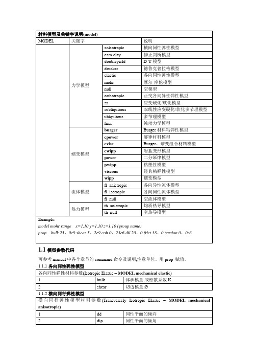
1.1模型参数代码可参考manual中各个章节的command命令及说明,注意单位。

用prop 赋值。

16 ttable 塑性拉应变-抗拉强度的表号下列参数可以显示、绘图与通过fish访问1 es_plastic 塑性切应变2 et_plastic 塑性拉应变3 ff_count 检测切应变反向的数4 ff_cvd 体应变,εvd经典粘弹性模型的材料参数(Classical Viscoelastic (Maxwell Substance) –MODEL mechanical viscous)1 bulk 弹性体积模量,K2 shear 弹性剪切模量,G3 viscosity 动力粘度,η粘弹性模型的材料参数(Burgers Model –MODEL mechanical burgers)1 bulk 弹性体积模量,K2 kshear Kelvin弹性剪切模量,G K3 kviscosity Kelvin动力粘度,ηK4 mkshear Maxwell切边模量,G M5 mviscosity Maxwell动力粘度,ηM二分幂律模型的材料参数(Power Law –MODEL mechanical power)1 a_1 常数,A12 a_2 常数,A23 bulk 弹性体积模量,K4 n_1 指数,n15 n_2 指数,n26 rs_1 参考应力,σ1ref7 rs_2 参考应力,σ2ref8 shear 弹性剪切模量,G蠕变模型材料参数(WIPP Model –MODEL mechanical wipp)1 act_energy 活化能,Q2 a_wipp 常数,A3 b_wipp 常数,B4 bulk 弹性体积模量,K5 d_wipp 常数,D6 e_dot_star临界稳定状态蠕变率,7 gas_c 气体常数,R8 n_wipp 指数,n9 shear 弹性剪切模量,G10 temp 温度,T下列参数可以显示、绘图与通过fish访问1 e_prime 累积主蠕变应变2 e_rate 累积主蠕变应变率Burger、蠕变组合材料模型的材料参数(Burgers-Creep Viscoplastic Model –MODEL mechanical cvisc)1 bulk 弹性体积模量,K2 cohesion 内聚力,c3 density 密度,ρ4 dilation 剪胀角,Ψ5 friction 内摩擦角,Φ6 kshear Kelvin弹性剪切模量,G K7 kviscosity Kelvin粘度,ηK8 shear 弹性剪切模量,G9 tension 抗拉强度,σt10 mviscosity Maxwell动力粘度,ηM下列计算参数可以显示、绘图与通过fish访问1 es_plastic 累积塑性切应变2 et_plastic 累积塑性拉应变幂律模型的材料参数(Power-Law Viscoplastic Model –MODEL mechanical cpower)1 a_1 常数,A12 a_2 常数,A23 bulk 弹性体积模量,K4 cohesion 内聚力,c5 dilation 剪胀角,Ψ6 friction 内摩擦角,Φ7 n_1 指数,n18 n_2 指数,n29 rs_1 参考应力,σ1ref10 rs_2 参考应力,σ2ref11 shear 弹性剪切模量,G12 tension 抗拉强度,σt粘塑形模型的材料参数(WIPP-Creep Viscoplastic Model –MODEL mechanical pwipp)1 act_energy 活化能,Q2 a_wipp 常数,A3 b_wipp 常数,B4 bulk 弹性体积模量,K5 d_wipp 常数,D6 e_dot_star临界稳定状态蠕变率,7 gas_c 气体常数,R8 kshear 材料参数,KΦ9 n_wipp 指数,n10 kdil 材料参数,q k11 kvol 材料参数,qΦ12 shear 弹性切变模量,G13 temp 温度,T14 tension 抗拉强度,σt以下计算参数可以显示、绘图与通过fish访问1 e_prime 累积主蠕变应变2 e_rate 累积主蠕变应变率3 es_plastic 累积塑性切应变4 et_plastic 累积塑性拉应变碎盐变形模型的材料参数(Crushed-Salt Model –MODEL mechanical cwipp)1 act_energy 活化能,Q2 a_wipp 常数,A3 b_f 最终体积模量,K f4 b_wipp 常数,B5 b0 蠕变压实系数,B06 b1 蠕变压实系数,B17 b2 蠕变压实系数,B28 bulk 弹性体积模量,K9 d_f 最终密度,ρf10 d_wipp 常数,D11 e_dot_star临界稳定状态蠕变率,12 gas_c 气体常数,R13 n_wipp 指数,n14 rho 密度,ρ15 s_f 最终切变模量,G f16 shear 弹性切变模量,G17 temp 温度,T以下计算参数可以显示、绘图与通过fish访问1 frac_d 当前碎片密度,ρd2 s_g1 蠕变压实参数,G3 s_k1 蠕变压实参数,K均质流体模型的材料参数1 permeability 等方向渗透性,k2 porosity 孔隙率,n(默认时,n=0、5)各向异性流体模型的材料参数1 fdd k1-k2的平面倾向2 fdip k1-k2的平面倾角1.2模型适用说明遍布节理模型适用于Mohr-Coulomb材料来明确显示力在各个方向上的差异性。

材料模型及关键字说明（model）MODEL关键字说明力学模型anisotropic横向同性弹性模型cam-clay修正剑桥模型doubleyield D-Y模型drucker德鲁克普拉格模型elactic各向同性弹性模型mohr摩尔-库伦模型null空模型orthotropic正交各向异性弹性模型ss应变硬化/软化模型subliquitous双线性应变硬化/软化多节理模型ubiquitous多节理模型finn纯动力学模型蠕变模型burger Burger材料粘弹性模型cpower幂律材料模型cvisc Burger、蠕变组合材料模型cwipp岩盐变形模型power二分幂律模型pwipp粘塑性模型viscous经典粘弹性模型wipp蠕变模型流体模型fl_anistropic各向异性流体模型fl_isotropic各向同性流体模型fl_null空流体模型热力模型th_anistropic均质热导模型th_null空热导模型Example:model mohr range x=1,10 y=1,10 z=1,10 （group name）prop bulk 25.0e9 shear 5.2e9 coh 0.23e6 dil 20.0 frict 38.0 tension 0.0e61.1模型参数代码可参考manual中各个章节的command命令及说明，注意单位。

用prop 赋值。

各向同性弹性材料参数（Isotropic Elastic – MODEL mechanical elastic）1bulk体积模量，或松散系数K2shear切边模量，G横向同行弹性模型材料参数（Transversely Isotropic Elastic – MODEL mechanical anisotropic）1dd同性平面的倾向2dip同性平面的倾角3e1同性平面的弹性模量4e3垂直同性平面的弹性模量5g12切变模量6nu12同性平面内施力时的泊松比7nu13垂直同性平面内施力时的泊松比正交各向异性弹性模型正交各向异性弹性模型材料参数（Orthotropic Elastic – MODEL mechanical orthotropic）1dd轴1-‘2’所定义平面的倾向2dip轴1-‘2’所定义平面的倾角3e11’方向弹性模量4e22’方向弹性模量5e33’方向弹性模量6g12平行于轴1-‘2’平面的切变模量7g13平行于轴1-‘3’平面的切变模量8g23平行于轴2-‘3’平面的切变模量9nu12沿2’方向施力，1’方向的泊松比10nu13沿3’方向施力，1’方向的泊松比11nu23沿3’方向施力，2’方向的泊松比12nx轴1-‘2’所定义平面单位法线x分量13ny轴1-‘2’所定义平面单位法线y分量14nz轴1-‘2’所定义平面单位法线z分量15rot旋转角德鲁克-普拉格模型德鲁克-普拉格模型的材料参数（Drucker-Prager – MODEL mechanical drucker）1bulk弹性体积模量，K2ksnear材料参数，kφ3qdil材料参数，qφ4qvol材料参数，qΨ5shear弹性切变模量，K6tension抗拉强度，σt摩尔-库伦模型摩尔-库伦模型的材料参数（Mohr-Coulomb – MODEL mechanical mohr）1bulk弹性体积模量，K2cohesion内聚力，c3dilation剪胀角，Ψ4friction内摩擦角，Φ5shear弹性切边模量，G6tension抗拉强度，σt多节理模型的材料参数（Ubiquitous-Joint – MODEL mechanical ubiquitous）1bulk弹性体积模量，K2cohesion内聚力，c3dilation剪胀角，Ψ4friction内摩擦角，Φ5jcohesion节理内聚力，c j6jddirection弱面dip方向（倾向）7jdilation节理剪胀角，Ψj8jdip弱面dip角度（倾角）9jfriction节理摩擦角，Φj10jnx弱面单位法线x分量11jny弱面单位法线y分量12jnz弱面单位法线z分量13jtension抗拉强度，σsj14shear弹性切边模量，G15tension抗拉强度，σt应变硬化/软化模型应变硬化/软化模型的材料参数（Strain-Hardening/Softening – MODEL mechanical ssoftening）1bulk弹性体积模量，K2cohesion内聚力，c3ctable塑性剪切应变-内聚力的表号4diation剪胀角，Ψ5dtable塑性剪切应变-剪胀角的表号6friction内摩擦角，Φ7ftable塑性剪切应变-摩擦角的表号8shear弹性切边模量，G9tension抗拉强度，σs10ttable塑性剪切应变-抗拉强度的表号双线性应变硬化/软化多节理模型的材料参数（Bilinear Strain-Hardening/Softening Ubiquitous-Joint –MODEL mechanical subiquitous）1bijoint=0，为线性节理，默认=1，为双线性节理2bimatrix=0，线性矩阵=1，双线性矩阵3bulk弹性体积模量，K4c2table塑性剪切应变-内聚力c2的表号5cjtable节理塑性剪切应变-节理内聚力c j1的表号6cj2table节理塑性剪切应变-节理内聚力c j2的表号7cohesion内聚力，c18co2内聚力，c29ctable塑性剪切应变-内聚力c1的表号10d2table塑性剪切应变-剪胀角Ψ2的表号11di2剪胀角，Ψ212dilation剪胀角，Ψ113djtable节理塑性剪切应变-节理剪胀角Ψj1的表号14dj2table节理塑性剪切应变-节理剪胀角Ψj2的表号15dtable塑性剪切应变-剪胀角Ψ1的表号16f2table塑性剪切应变-摩擦角Φ2的表号17fjtable节理塑性剪切应变-节理摩擦角Φj1的表号18fj2table节理塑性剪切应变-节理摩擦角Φj2的表号19fr2摩擦角Φ220friction摩擦角Φ121ftable塑性剪切应变-摩擦角Φ1表号22jc2节理内聚力c j123jcohesion节理内聚力c j224jddirection弱面dip方向（倾向）25jdilation节理剪胀角Ψj126jdip弱面dip角度（倾角）27jd2节理剪胀角，Ψj128jfriction节理摩擦角，Φj129jf2节理摩擦角，Φj230jnx弱面单位法线x分量31jny弱面单位法线y分量32jnz弱面单位法线z分量33jtension节理抗拉强度，σsj34shear弹性切边模量，G35tension抗拉强度，σs36tjtable节理塑性剪切应变-节理抗拉强度σtj的表号37ttable节理塑性剪切应变-节理抗拉强度σt的表号下列参数可以显示、绘图或者fish访问1es_plastic塑性切应变2et_plastic塑性拉应变3etj_plastic节理塑性拉应变4esj_plastic节理塑性切应变D-Y模型的材料参数（Double-Yield – MODEL mechanical doubleyield）1bulk弹性体积模量，K2cap_pressure cap压力，p c3cohesion内聚力，c4cptable塑性体应变-cap压力的表号5ctable塑性切应变-内聚力的表号6dilation剪胀角，Ψ7dtable塑性切应变-剪胀角的表号8ev_plastic塑性体应变总量9friction内摩擦角，Φ10ftable塑性切应变-摩擦角的表号11multiplier当前塑性-cap模量与弹性体积和切变模量的倍数，R12shear最大弹性切变模量，G13tension抗拉强度，σs14ttable塑性拉应变-抗拉强度的表号下列计算参数可以显示、绘图和通过fish访问1es_plastic累积塑性切应变2et_plastic累积塑性拉应变3ev_plastic累积塑性体应变修正剑桥模型修正剑桥模型的材料参数（Modified Cam-Clay – MODEL mechanical cam-clay）1bulk_bcund最大的弹性体积模量，K max2cv初始容积，v c3kappa弹性膨胀线斜率，k4lamda常态固结线斜率，λ5mm摩擦常数，M6mpc预固结压力，p c07mp1预固结压力，p18mv_1指定在参考压力常态固结线的容积v A 9poisson泊松比，ν10shear弹性剪切模量，G下列参数可以显示、绘图以及fish访问1bulk体积模量，K2cam_cp当前平均有效应力3cam_ev累积总容积应变4camev_cp累积塑性容积应变5cq当前平均差分应力纯动力学模型的材料参数（config dynamic, model mech finn）1bulk弹性体积模量，K2cohesion内聚力，c3ctable弹性切应变-内聚力的表号4dilation剪胀角，Ψ5dtable塑性切应变-剪胀角Ψ的表号6ff_c1常量，c17ff_c2常量，c28ff_c3常量，c39ff_c4常量，c410ff_latensy反向之间的最小时间步数11ff_switch=0：Martin（1995）公式=1：Byme（1991）公式12friction内摩擦角，Φ13ftable塑性切应变-摩擦角的表号14shear最大弹性切变模量，G15tension抗拉强度，σt16ttable塑性拉应变-抗拉强度的表号下列参数可以显示、绘图和通过fish访问1es_plastic塑性切应变2et_plastic塑性拉应变3ff_count检测切应变反向的数4ff_cvd体应变，εvd经典粘弹性模型经典粘弹性模型的材料参数（Classical Viscoelastic （Maxwell Substance）– MODEL mechanical viscous）1bulk弹性体积模量，K2shear弹性剪切模量，G3viscosity动力粘度，η粘弹性模型粘弹性模型的材料参数（Burgers Model – MODEL mechanical burgers）1bulk弹性体积模量，K2kshear Kelvin弹性剪切模量，G K3kviscosity Kelvin动力粘度，ηK4mkshear Maxwell切边模量，G M5mviscosity Maxwell动力粘度，ηM二分幂律模型二分幂律模型的材料参数（Power Law – MODEL mechanical power）1a_1常数，A12a_2常数，A23bulk弹性体积模量，K4n_1指数，n15n_2指数，n26rs_1参考应力，σ1ref7rs_2参考应力，σ2ref8shear弹性剪切模量，G蠕变模型材料参数（WIPP Model – MODEL mechanical wipp）1act_energy活化能，Q2a_wipp常数，A3b_wipp常数，B4bulk弹性体积模量，K5d_wipp常数，D6e_dot_star临界稳定状态蠕变率，ϵ̇ss∗7gas_c气体常数，R8n_wipp指数，n9shear弹性剪切模量，G10temp温度，T下列参数可以显示、绘图和通过fish访问1e_prime累积主蠕变应变2e_rate累积主蠕变应变率Burger、蠕变组合材料模型Burger、蠕变组合材料模型的材料参数（Burgers-Creep Viscoplastic Model – MODEL mechanical cvisc）1bulk弹性体积模量，K2cohesion内聚力，c3density密度，ρ4dilation剪胀角，Ψ5friction内摩擦角，Φ6kshear Kelvin弹性剪切模量，G K7kviscosity Kelvin粘度，ηK8shear弹性剪切模量，G9tension抗拉强度，σt10mviscosity Maxwell动力粘度，ηM下列计算参数可以显示、绘图和通过fish访问1es_plastic累积塑性切应变2et_plastic累积塑性拉应变幂律模型幂律模型的材料参数（Power-Law Viscoplastic Model – MODEL mechanical cpower）1a_1常数，A12a_2常数，A23bulk弹性体积模量，K4cohesion内聚力，c5dilation剪胀角，Ψ6friction内摩擦角，Φ7n_1指数，n18n_2指数，n29rs_1参考应力，σ1ref10rs_2参考应力，σ2ref11shear弹性剪切模量，G12tension抗拉强度，σt粘塑形模型的材料参数（WIPP-Creep Viscoplastic Model – MODEL mechanical pwipp）1act_energy活化能，Q2a_wipp常数，A3b_wipp常数，B4bulk弹性体积模量，K5d_wipp常数，D6e_dot_star临界稳定状态蠕变率，ϵ̇ss∗7gas_c气体常数，R8kshear材料参数，KΦ9n_wipp指数，n10kdil材料参数，q k11kvol材料参数，qΦ12shear弹性切变模量，G13temp温度，T14tension抗拉强度，σt以下计算参数可以显示、绘图和通过fish访问1e_prime累积主蠕变应变2e_rate累积主蠕变应变率3es_plastic累积塑性切应变4et_plastic累积塑性拉应变碎盐变形模型碎盐变形模型的材料参数（Crushed-Salt Model – MODEL mechanical cwipp）1act_energy活化能，Q2a_wipp常数，A3b_f最终体积模量，K f4b_wipp常数，B5b0蠕变压实系数，B06b1蠕变压实系数，B17b2蠕变压实系数，B28bulk弹性体积模量，K9d_f最终密度，ρf10d_wipp常数，D11e_dot_star临界稳定状态蠕变率，ϵ̇ss∗12gas_c气体常数，R13n_wipp指数，n14rho密度，ρ15s_f最终切变模量，G f16shear弹性切变模量，G17temp温度，T以下计算参数可以显示、绘图和通过fish访问1frac_d当前碎片密度，ρd2s_g1蠕变压实参数，G3s_k1蠕变压实参数，K均质流体模型均质流体模型的材料参数1permeability等方向渗透性，k2porosity孔隙率，n（默认时，n=0.5）各向异性流体模型的材料参数1fdd k1-k2的平面倾向2fdip k1-k2的平面倾角3frot k1轴和倾角矢量的转角4h1k1方向的渗透性5h2k2方向的渗透性6h3k3方向的渗透性均质热导模型的材料参数1conductivity等方向传热系数，K2spec_heat比热容，C v1.2模型适用说明遍布节理模型适用于Mohr-Coulomb材料来明确显示力在各个方向上的差异性。

Flac3D5.0教程第⼆章完成第⼀个简单分析计算样例by typing the commands from the keyboard, pressingat the end of each command line, and seeing the results directly.newgen zone brick size 6 8 8（This command will create an initial mesh that is six zones in the x-direction, eight zones in the y-direction and eight zones in the z-direction. For our model, the z-axis is oriented in the verticaldirection.）Plot（the Plot Base/0>prompt will appear. As long as this prompt appears, any subsequentcommands will be associated with the PLOT command. The plot view is identified as Base/0,which is the default view.）create Trenchadd surface yellowadd axes blackshowNow, give the zones a material model and properties. For this example, we use the Mohr-Coulombelastic-plastic model. Go back to the Flac3D>prompt in the command window andtype in thefollowing command:modelmohrThis will specify the Mohr-Coulomb model. Every zone in the grid could conceivably have adifferent material model and property. However, by not specifying a range of zonesafter the MODEL command, FLAC3D assumes that all zones are to be Mohr-Coulomb material.prop bulk = 1e8 shear = 0.3e8 fric = 35propcoh = 1e10 tens = 1e10You see that very high cohesion and tensile strength values are given. These areonlyinitial values that are used during the development of gravitational stresses within the body.In effect, we are forcing the body to behave elastically during the development of theinitial insitustress state.* This prevents any plastic yield during the initial loading phase of theanalysis.For this problem, loading is due to gravity. To apply gravity, use the commands setgrav 0, 0, -9.81ini dens = 1000In order to develop a gravitational body force, themass density must also be initialized. The INI command is used to initialize the mass density to1000 kg/m3 for all zones in the model.Next, the boundary conditions for the problem are set. At the Flac3D>prompt, type fix x range x -0.1 0.1fix x range x 5.9 6.1fix y range y -0.1 0.1fix y range y 7.9 8.1fix z range z -0.1 0.1With these commands, roller boundaries are placed on five sides of the model. The boundaries are “fixed” only in the specified direction (i.e., no displacement or velocity is allowed). The FIX commands perform the following functions.1. The gridpoints along the boundary planes at x = 0 and x = 6 are fixed in the x-direction. These two planes fall within the coordinate ranges specified by the range keywords for the first two FIX commands.2. The gridpoints along the boundary planes at y = 0 and y = 8 are fixed in the y-direction. These planes fall within the ranges specified for the third and fourth FIX commands.3. The gridpoints along the bottom boundary (z = 0) are fixed in the z-direction. This plane falls within the range for the fifth FIX command.We wish to monitor the change in the values of selected variables in the model during the calculational stepping. A HISTORY command can assist in helping us determinewhether a stable equilibrium solution or unstable collapse is occurring. We type the following commands:hist n = 5histunbalhistgpzdisp 4,4,8We choose to monitor the change in variables every five calculation steps. It is always a good idea to monitor the maximum unbalanced force in a model. If the unbalanced force approaches a very small value and displacement histories become constant, this indicates that an equilibrium state is reached.To allow gravitational stresses to develop within the body, we timestep the simulation to equilibrium.Here the SOLVE command is used to detect equilibrium automatically.setmech force=50solveWhen the unbalanced force falls below the limiting value (a limiting force of 50 N is specified with the SET command), the run will stop.* The plots are updated, since they are still visible on the screen. Shutting down the plots will cause the model to cycle faster.plothist 1hist 2The unbalanced force history approaches zero, andthe displacement history becomes constant; both are indicators that an equilibriumstate has beenreached.Note that each history is numbered sequentially from 1 as it is entered via the HIST command. Return to the Flac3D> prompt and typeprinthistfor a listing of the histories and their corresponding numbers.Plotcreat trenchadd contour dispadd axes blackshowclearaddbcontourszzadd axesplot create GravVplot set plane dip=90 dd=0 origin=3,4,0plot set rot 15 0 20plot set center 2.5 4.2 4.0plot add bound behindplot add bcontszz planeplot add axesplot showThis sequence will create a view, which we have called GravV, and make it the current view. We then set a plane for that view oriented at a dip angle of 90? (from the xy-plane, assuming that negative-z is “down”), a dip direction of 0?(measured clockwise from the positive y-axis in the xy-plane) and with one point on the plane at (x = 3, y = 4, z = 0). We add a wire-frame boundary plotted behind the plane and a block contour plot of the vertical stress component, σzz, on the plane. Finally, the model axes are added. The block contour plot, as opposed to an interpolated contour plot, displays the value of the stress calculated at each zone centroid. The color of each zone corresponds directly to the zone-based stress.It is wise to save the initial state so that you can restore it at any time to perform parameter studies.savetrench.savWe can change the current view from GravV to Trench with the commandplot current TrenchNow we can excavate a trench in the soil. First, typepropcoh=1e3 tens=1e3This will set the cohesion and tensile strength for all zones to 1000 Pa. These valuesfor strength arehigh enough to prevent failure in our initial state (i.e., unexcavated), but you shouldalways checkfor possible failure in the initial state by performing a few calculation steps. Toexcavate the trench,entermodel null range x=2,4 y=2,6 z=5,10With a low cohesion and vertical unsupported trench walls, collapse should occur. Because wewant to examine this process realistically, the large-strain logic is specified. This isdone by typingset largeFor plotting purposes, we wish to see only the change in displacements from the trench excavation, and not from the previous gravitational loading, so we zero out the x-, y- and z-displacement components:inixdis=0 ydis=0 zdis=0We purposely set the cohesion low enough to result in failure, so we do not want to use the SOLVE command with a limit for out-of-balance force (which checks for equilibrium). Oursimulation willnever converge to the equilibrium state. Instead, we can step through the simulationprocess onetimestep at a time, and plot and print the results of the collapse as it occurs. This is thereal powerof the explicit method. The model is not required to converge to equilibrium at eachcalculationcycle because we never have to solve a set of linear algebraic equationssimultaneously, as is thecase for implicit codes, with which many engineers are familiar.we use the STEP command: step 2000第三章FLAC 3D基础知识gridpointzonehorizontal boundary stressstructural cables(tiebacks)model boundaryinternal boundaries(excavation)roller bottom boundaryNamed ObjectsMacro Object—Typically, such an object contains a long, complex string that may be used repeatedly in the model. The pre-processor compares a string of command tokens to the list of defined macros and replaces any matching macro object with its fully expanded contents.macro Pt0 ’p0 0 0 0’macro Pt1 ’p1 add 10 0 0’macro Pt2 ’p2 add 0 10 0’macro Pt3 ’p3 add 0 0 10’macroModel_Size ’size 4 5 6’macroBig_Brick ’zone brick Pt0 Pt1 Pt2 Pt3 Model_Size’.genBig_Brick.macro ’Pt0’ ’p0 15 15 15’genBig_BrickThis pre-processing has two effects:(1) macro objects may be nested (but not recursively); and(2) the macro object name is removed from the command string.Model Object—Model objects, such as ranges in space, groups of zones in a model, or plot views, can be given userdefined names. Those objects can then be referred to by their names.gen zone brick size 6 6 6group Tunnel range x 1 5 y 0 6 z 1 5modelmohr..modelnul range group Tunnel.The named range and the named group are two very different model objects. The range pertains toa specified volume of space (or range of values), whereas the group identifies acollection of finitedifference zones in the model.Sign ConventionsDIRECT STRESS —Positive stresses indicate tension; negative stresses indicate compression.第四章初级实体建模技术Grid generation is performed via the GENERATE command and associated keywords that both define the number of zones in a model and shape the grid to fit a specified problem region.The number of zones is specified by the size keyword.It is best to start with a grid that has few zones (say, 1000 to 1500) to perform simple test runs andmake refinements to the grid. Then, increase the number of zones to improve theaccuracy.Using actual coordinatesgen zone brick size 6,8,8 p0 -10, -10, -20 &p1 10, -10, -20 &p2 -10, 10, -20 &p3 -10, -10, 0plot surfOnly four corners are required to define a parallelepiped-shaped mesh. More corners can be specifiedto define an irregular surface. Example 2.14 shows how to make a sloping surface atthe top of themesh.gen zone brick size 6,8,8 p0 -10, -10, -20 &p1 10, -10, -20 p2 -10, 10, -20 &p3 -10, -10, 0 p4 10, 10, -20 &p5 -10, 10, 10 p6 10, -10, 0 &p7 10, 10, 10plot surfIn the tutorial example, we noted that the boundaries of the model were influencing the results (see Figure 2.6). The boundary must be placed far enough away from the excavation to reduce these effects. A gradually graded mesh can be created in FLAC3D to move the model boundaries farther out without significantly increasingthe number of zones. For example, the command GEN zone radbrick creates a radially graded mesh around a brick-shaped mesh. The command in Example 2.15 creates a 3 ×5 ×5 zone brick-shaped mesh surrounded by a 7-zone radially graded mesh.gen zone radbrick&p0 (0,0,0) p1 (10,0,0) p2 (0,10,0) p3 (0,0,10) &size 3,5,5,7 &ratio 1,1,1,1.5 &dim 1 4 2 fillplot surfThe x,y,z coordinate system in FLAC3D is always right-handed and, as a default, the z-axis is drawn in the vertical direction on the screen. In Example 2.14 we assumed the z-axis was pointing in the vertical direction. However, we do not have to interpret the z-axis to mean the up direction. For Example 2.15, we will assume that the y-axis is the vertical direction. As long as we define the model in a right-handed system, we can create the grid in any direction we desire.The size keyword, as used in Example 2.15, specifies the number of zones in the brick and the number radially surrounding the brick (see Figure 2.11). The keyword ratio is given to manipulate the grid spacing. The four values that follow ratio are geometric ratios between successive zone sizes. The first three values are ratios for the zones in the brick, and the fourth value is the ratio for the zones surrounding the brick. In Example 2.15 above, the ratio is 1.0 for the brick zones and1.5 for the zones surrounding the brick. This causes each successive ring of zones surrounding the brick to be 1.5 times larger in the radial direction. The dim keyword defines the dimensions of the brick region (i.e., 1 m ×4 m ×2 m). The fill keyword fills the brick region with zones. If fill is omitted, no zones will be generated within the brick region.Notice that size, ratio and dim all refer to local axes as defined by p0, p1, p2, p3 in Figure 2.11, not to the global x,y,z-axes.Creating a model by reflecting elements on planes of symmetrygen zone radbrick&p0 (0,0,0) p1 (10,0,0) p2 (0,10,0) p3 (0,0,10) &size 3,5,5,7 &ratio 1,1,1,1.5 &dim 1 4 2 fillgen zone reflect dip 0 dd 90gen zone reflect dip 90 dd 90plot surfdip 为倾⾓的意思，其值⼤⼩为⾯与xy⾯所夹的倾⾓，dd为倾向，其值⼤⼩为⾯的法线在xy平⾯上的投影与y轴的夹⾓。