Q-方程,弹性散射运动学lec16

弹性散射与费弹性散射散射简介1、瑞利散射是一种由热力学涨落（如密度温度）所引起的弹性散射。

在固体中这种效应被缺陷和杂质的散射所掩盖，在流体中明显一些。

入射光在线度小于光波长的微粒上散射后散射光和入射光波长相同的现象。

由英国物理学家瑞利提出而得名。

分子散射光的强度与入射光的频率的四次方成正比。

瑞利散射公式为I (θ)2 =πd λ-4R -2V 2(1+cos2θ)(n -1) I 0其中d 为散射粒子数，V 是粒子的提及，n 是折射率，θ是入射线与散射线之间的夹角，称为散射角。

波长愈短的电磁波，散射愈强烈，当电磁波波长大于1毫米时，瑞利散射可以忽略不计。

瑞利，英国人，十九世纪最著名的物理学家之一，1904年，他因和拉姆塞同时发现了惰性元素氩（Ar ）而荣获了该年度的诺贝尔物理学奖。

非弹性散射射包括布里渊散射和拉曼散射。

2、布里渊散射它是由于声波通过介质时所引起的折射率不均匀而产生的当波长较短的压缩波(例如声波) 穿越固体或液体媒质时，引起的光的散射现象。

声波穿过媒质，将使媒质中存在以声速传播的压强起伏，引起媒质各处密度的起伏，从而产生对可见光的散射现象。

这种散射光的频率ν较入射光频率ν0有一个频移，ν-ν0，但其值很小，远小于喇曼散射的频移，且频移与散射角有关。

布里渊散射为美籍物理学家L. 布里渊1922年首先研究在不同条件下，布里渊散射又分自发散射和受激散射两种形式光纤中的布里渊散射在注入光功率不高的情况下，光纤材料分子的布朗运动将产生声学噪声，当这种声学噪声在光纤中传播时，其压力差将引起光纤材料折射率的变化，从而对传输光产生自发散射作用，同时声波在材料中的传播将使压力差及折射率变化呈现周期性，导致散射光频率相对于传输光有一个多普勒频移，这种散射称为自发布里渊散射。

自发布里渊散射可用量子物理学解释如下：一个泵浦光子（注入光纤中的信号光）转换成一个新的频率较低的斯托克斯光子并同时产生一个新的声子；同样地，一个泵浦光子吸收一个声子的能量转换成一个新的频率较高的反斯托克斯光子。

中子物理讲义（研究生讲座教材）兰州大学物理学院王学智目录绪言第一章Q方程及其应用§1 核反应和反应道§2 Q方程的推导§3 反应阈能和临界能量§4 Q方程的应用§5 L系和C系的出射角转换第二章中子源物理§1 中子产生§2 同位素中子源§3 加速器中子源§4 常用加速器中子源§5 反应堆中子源第三章中子与物质的相互作用§1 基本物理量§2 核反应机制§3 中子与物质相互作用的物理过程第四章中子测量技术§1 长中子计数器§2 伴随粒子法§3 望远镜§4 裂变室§5 活化探测器第五章中子剂量测量方法§1 基本概念§2 中子雷姆仪§3 （n，γ）混合场的吸收剂量测量第六章中子能谱测量§1 反冲质子法§2 特种核乳胶法§3 阈能探测器法§4 中子TOF谱仪§5 聚变中子测温第七章辐射防护问题§1 γ的屏蔽§2 中子屏蔽第八章宏观中子物理§1 中子减速和热化§2 中子在物质中的空间分布§3 多组理论绪言1932年英国人Chachwick 发现中子，这是20世纪物理学发展中的重大事件，它与人工放射性、带电粒子加速技术并列为30年代的原子核研究的三个里程碑。

中子应用于研究物质结构的各门学科中，不仅引起核物理研究的质的飞跃，而且因建立原子核有质子与中子通过强相互作用构成的量子多体体系的认识以及对介子场理论研究和实验研究的深入，并促进粒子物理学发展。

中子应用促进了一系列交叉学科的发展。

核裂变现象不仅为核物理开辟了一个重要分支领域，而且进一步促进核物理－化学的紧密结合－核化学分支。

中子作为改造自然界的工具，在工业、技术、材料、资源等方面的应用，对社会发展、经济增长产生极为广泛的影响。

弹性波散射现象的数值模拟与分析引言弹性波散射是指当弹性波在遇到不同介质或物体边界时发生的反射、折射和散射现象。

研究弹性波散射现象对于地震勘探、地质灾害预测以及材料科学等领域具有重要意义。

本文将介绍弹性波散射现象的数值模拟与分析方法，以及其在实际应用中的意义和挑战。

一、数值模拟方法1. 有限差分法有限差分法是一种常用的数值模拟方法，适用于求解弹性波方程。

该方法将连续的空间和时间离散化，通过有限差分近似来求解偏微分方程。

有限差分法简单易行，适用于各种边界条件和复杂介质情况。

然而，由于网格剖分的限制，有限差分法对于大尺度、高频率的问题计算量较大。

2. 有限元法有限元法是一种基于离散化方法的数值模拟方法，适用于求解各种复杂边界条件和非均匀介质情况下的弹性波散射问题。

该方法将连续的物理域分割成有限个小单元，通过插值函数和基函数来逼近解的形式。

有限元法具有较高的计算精度和灵活性，但对于大规模问题的计算量较大。

3. 边界元法边界元法是一种基于边界积分方程的数值模拟方法，适用于求解边界上的弹性波散射问题。

该方法通过将边界上的积分方程离散化，将问题转化为求解线性方程组的形式。

边界元法适用于各种复杂边界条件和介质情况，具有高效的计算速度和较小的存储需求。

二、数值模拟与实际应用1. 地震勘探地震勘探是一种通过观测地震波在地下传播和散射的信息来获取地下结构和物性的方法。

数值模拟可以帮助预测地震波在地下的传播路径和散射特性，从而指导地震勘探的设计和解释。

通过模拟不同介质和地下结构的散射现象，可以提高地震勘探的效率和准确性。

2. 地质灾害预测地质灾害预测是一种通过分析地下介质和构造的变化来预测地质灾害风险的方法。

数值模拟可以模拟地震波在地下的传播和散射过程，从而帮助预测地质灾害的发生概率和影响范围。

通过模拟不同地质条件下的散射现象，可以提高地质灾害预测的准确性和可靠性。

3. 材料科学材料科学是一门研究材料性质和结构的学科，对于材料的弹性波散射现象的研究具有重要意义。

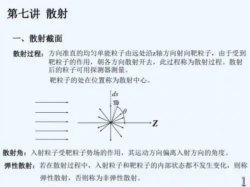
第七讲散射理论一、散射现象的一般描述1、什么是散射？简单地说，散射就是指粒子与粒子之间或粒子与力场之间的碰撞（相互作用）过程，是一种具有重要实际意义的现象，所以散射现象也称碰撞现象，其可以示意为：粒子流散射中心如：原子物理中的α粒子散射实验。

2、散射的分类：弹性散射：一粒子与另一粒子碰撞的过程中，只有动能的交换，粒子内部状态并无改变。

非弹性散射：两粒子碰撞中粒子的内部状态有所改变（例如原子被激发或电离）。

在这里我们只讨论弹性散射，即假设碰撞过程中粒子的内部状态未变，并假设散射中心质量很大、碰撞对其运动没有影响。

3、散射的经典力学描述从经典力学来看，在散射过程中，每个入射粒子都以一个确定的碰撞参数（瞄准距离）b 和方位角0ϕ射向靶子，由于靶子的作用，入射粒子的轨道将发生偏转，沿某方向(,)θϕ出射。

例如在α粒子的散射实验中，有22cot 422M b Ze θυπε= （偏转角θ与瞄准距离之间的关系） 那些瞄准距离在b b db -和之间的α粒子，散射后，必定向着d θθθ+和之间的角度射出，如下图所示：凡通过图中所示环形面积d σ的α粒子，必定散射到角度在d θθθ+和之间的一个空心圆锥体之中。

环形面积d σ称为有效散射截面，又称微分截面。

且2222401()()4sin 2Ze d d M σθπευΩ= 然而，在散射实验中，人们并不对每个粒子的轨道感兴趣，而是研究入射粒子束经过散射后沿不同方向出射的分布。

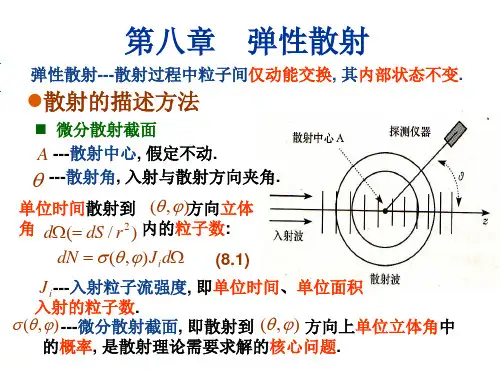
设一束粒子流以稳定的入射流强度沿Z 轴方向射向靶粒子A ，由于靶粒子的作用，设在单位时间内有dn 个粒子沿(,)θϕ方向的立体角d Ω中射出，显然，,(,)dn Nd dn q Nd θϕ∝Ω=Ω令，即1(,)()dn q N d θϕ=Ω显然，(,)q θϕ具有面积的量纲，称为微分散射截面。

微分散射截面),(ϕθq 表示单位时间内散射到单位立体角Ωd （面积/距离平方）的粒子数占总粒子数比率，即Ω=Nd q dn ),(ϕθ。

_______________________________________________________________________ ________________________________________________________________________22.101 Applied Nuclear Physics (Fall 2004)Lecture 16 (11/12/04)Neutron Interactions: Q-Equation, Elastic ScatteringReferences :R. D. Evan, Atomic Nucleus (McGraw-Hill New York, 1955), Chap. 12.W. E. Meyerhof, Elements of Nuclear Physics (McGraw-Hill, New York, 1967), Sec. 3.3. Since a neutron has no charge it can easily enter into a nucleus and cause reaction. Neutrons interact primarily with the nucleus of an atom, except in the special case of magnetic scattering where the interaction involves the neutron spin and the magnetic moment of the atomic. Since we will not consider magnetic scattering in this class we can neglect the interaction between neutrons and electrons and think of atoms and nuclei interchangeably. Neutron reactions can take place at any energy, so one has to payparticular attention to the energy dependence of the interaction cross section. In a nuclear reactor neutrons with energies from 10-3 ev (1 mev) to 107 ev (10 Mev) are of interest, this means we will be covering an energy of 1010.For a given energy region – thermal, epithermal, resonance, fast – not all thepossible reactions are equally important. What reaction is important depends on the target nucleus and the neutron energy. Generally speaking the important types of interactions, in the order of increasing complexity from the standpoint of theoretical understanding, are:(n,n) – elastic scattering. There are two processes, potential scattering which is neutron interaction at the surface of the nucleus (no penetration) as in billiard ball-like collision, and resonance scattering which involves the format and decay of a compound nucleus.(n,γ) --radiative capture.(n,n’) --inelastic scattering. This reaction involves the excitation of nuclearlevels.(n,p), (n,α), … -- charged particle emission.(n,f) --fission.If we were interested in fission reactors, the reactions in the order of importance would be fission, capture (in fuel and other reactor materials), scattering (elastic and inelastic), fission product decay by β-emission as in decay neutrons and heat production. In this chapter we will mostly study elastic (or potential) scattering. The other reactions all involve compound nucleus formation, a process we will discuss briefly around the end of the semester.The Q-EquationConsider the reaction, sketched in Fig. 15.1, where an incoming particle (labeled 1) collides with a target nucleus (2), resulting in the emission of an outgoing particle (3), with the residual nucleus (4) recoiling. For simplicity we assume the target nucleus to beFig. 15.1. A two-body collision between incident particle 1 and target particle 2, which is at rest, leading to the emission of particle 3 at an angle θ and a recoiling residual particle 4.at rest, E2 = 0. This is often a good approximation because the target is at room temperature, which means E2 is 0.025 ev, and unless the incoming neutron is in the thermal energy region, E1 typically will be much greater than E2. We will derive an equation relating the outgoing energy E3 to the outgoing angle θ using the conservation of total energy and linear momentum, and non-relativistic kinematics,2M 2 ) (15.1)M 2) +(E + cM =(E + c(E + cM 2) + c1 1 23 3 4 4p =p + p (15.2)13 4 Rewriting the momentum equation as2p 4 = ( p 1 − p 3)2 2= p + p 2 − 2 p p cos θ= 2 E M 4 (15.3)131 3 4 and recalling)2Q = (M + M 2 − M − c M 1 3 4 =E 3 + E 4 − E 1(15.4)we obtain ⎛ M 3 ⎞⎛ ⎞ 2Q = E 3 ⎜⎜ 1 + ⎟⎟− E 1 ⎜⎜ 1 − M 1 ⎟⎟ − E E M M 3 cos θ(15.5)⎝ M 4 ⎠⎝ M 4 ⎠ M 4 13 1 which is known as the Q-equation. Notice that the energies E i and angle θ are in the laboratory coordinate system (LCS), while Q is independent of coordinate system (since Q can be expressed in terms of masses which of course do not depend on coordinate system). A typical situation is when the incident energy E 1, the masses (and therefore Q-value) are all known, and one is interested in solving (15.5) for E 3 in terms of cos θ , or vice versa.Eq. (15.5) is actually not an equation for determining the Q-value, since this is already known in the sense that all four particles in the reaction and their rest masses are prescribed beforehand. This being the case, what then is the quantity that one would solve (15.5) to obtain? We can think of the Q-equation as a relation connecting the 12 degrees of freedom in any two-body collision problem, where two particles collide (asreactants) to give rise to two other particles (as products). The problem is said to be completely specified when the velocities of the fours particles, or 12 degrees of freedom (each velocity has 3 degrees of freedom), are determined. Clearly not every single degree of freedom is a variable in the situations of interest to us. First of all the direction oftravel and energy of the incoming particle are always given, thus eliminating 3 degrees of freedom. Secondly it is customary to take the target nucleus to be stationary, so another 3 degrees of freedom are removed. Since conservation of energy and momentum must hold in any collision (three conditions since momentum and energy are related), this leaves three degrees of freedom in the problem. If we further assume the emission of the outgoing particle (particle 3) is azimuthally symmetric (that is, emission is equally probably into a cone subtended by the angle θ ), only two degree of freedom are left. What this means is that the outcome of the collision is completely determined if we just specify another degree of freedom. What variable should we take? Because we are often interested in knowing the energy or direction of travel of the outgoing particle, we can choose this last variable to be either E 3 or the scattering angle θ . In other words, if we know either E 3 or θ , then everything else (energy and direction) about the collision is determined. Keeping this in mind, it should come as no surprise that what we will do with (15.5) is to turn it into a relation between E 3 and θ .Thus far we have used non-relativistic expressions for the kinematics. To turn (15.5) into the relativistic Q-equation we can simply replace the rest mass M i by aneff 22effective mass, M i = M i + T i /2c , and use the expression p 2 =2MT + T / c 2 instead2of p 2 = 2ME . For photons, we take M eff = h ν/2c . Inspection of (15.5) shows that it is a quadratic equation in the variable x = E 3. An equation of the form ax 2 + bx + c = 0 has two roots,x ±=[− b ± b 24ac ]/2a (15.6)which means there are in general two possible solutions to the Q-equation, ± E 3. For a solution to be physically acceptable, it must be real and positive. Thus there aresituations where the Q-equation gives one, two, or no physical solutions [cf. Evans, pp. 413-415, Meyerhof, p. 178]. For our purposes we will focus on neutron collisions, in particular the case of elastic (Q = 0) and inelastic (Q < 0) neutron scattering. We will examine these two processes briefly and then return to a more detailed discussion of elastic scattering in the laboratory and center-of-mass coordinate systems.Elastic vs. Inelastic ScatteringElastic scattering is the simplest process in neutron interactions; it can beanalyzed in complete detail. This is an important process because it is the primarymechanism by which neutrons lose energy in a reactor, from the instant they are emitted as fast neutrons as a result of a fission event to when they appear as thermal neutrons. In this case, there is no excitation of the nucleus, Q = 0, whatever energy is lost by the neutron is gained by the recoiling target nucleus. Let M 1 = M 3 = m (M n ), and M 2 = M 4 = M = Am. Then (15.5) becomes⎛ 1 ⎞⎛ 1 ⎞ 2E 3 ⎜ 1 + ⎟− E 1 ⎜ 1 − ⎟− E E 3 cos θ= 0 (15.7)⎝ A ⎠⎝ A ⎠ A 1 Suppose we ask under what condition is E 3 = E 1? We see that this can occur only when θ = 0, which corresponds to forward scattering (no interaction). For all finite θ , E 3 has to be less than E 1. One can show that maximum energy loss by the neutron occurs at θ=π , which corresponds to backward scattering,⎛ A − 1⎞ 2E 3 = α E 1, α=⎜ ⎟ (15.8)⎝ A + 1⎠ Eq.(15.7) is the starting point for the analysis of neutron slowing down in a moderator medium. We will return to it later in this chapter.Inelastic scattering is the process by which the incoming neutron excites thetarget nucleus so it leaves the ground state and goes to an excited state at an energy E* above the ground state. Thus Q = -E* (E* > 0). We again let the neutron mass be m andthe target nucleus mass be M (ground state) or M* (excited state), with M* = M + E*/c 2. Since this is a reaction with negative Q, it is an endothermic process requiring energy to be supplied before the reaction can take place. In the case of scattering the only way energy can be supplied is through the kinetic energy of the incoming particle (neutron). Suppose we ask what is minimum energy required for the reaction, the threshold energy? To find this, we look at the situation where no energy is given to the outgoing particle, E 3 ~0 and θ ~ 0. Then (15.5) gives− E * − = E th ⎛⎜⎜ M 4 − M 1 ⎞⎟⎟ , orE th ~ E *(1+1/ A ) (15.9)⎝ M 4 ⎠ where we have denoted the minimum value of E 1 as E th . Thus we see the minimum kinetic energy required for reaction is always greater than the excitation energy of the nucleus. Where does the difference between E th and E* go? The answer is that it goes into the center-of-mass energy, the fraction of the kinetic energy of the incoming neutron (in the laboratory coordinate) that is not available for reaction.Relations between Outgoing Energy and Scattering AngleWe return to the Q-equation for elastic scattering to obtain a relation between the energy of the outgoing neutron, E 3, and the angle of scattering, θ . Again regarding (15.5) as a quadratic equation for the variable E 3 , we have2 A − 1E3 −E E 3 cos θ− E 1 = 0 (15.10)A + 1 1 A + 1 with solution in the form, 1/ 2 )E 3 = 1 E 1 (cos θ+[A 2 − sin 2 θ] (15.11)A + 1 This is a perfectly good relation between E 3 and θ (with E 1 fixed), although it is not a simple one. Nonetheless, it shows a one-to-one correspondence between these twovariables. This is what we meant when we said that the problem is reduced to only degree of freedom. Whenever we are given either E3 or θ we can immediately determine the other variable. The reason we said that (15.11) is not a simple relation is that we can obtain another relation between energy and scattering angle, except in this case the scattering angle is the angle in the center-of-mass coordinate system (CMCS), whereas θis the scattering angle in the laboratory coordinate system (LCS). To find this simpler relation we first review the connection the two coordinate systems.Relation between LCS and CMCSSuppose we start with the velocities of the incoming neutron and target nucleus, and those of the outgoing neutron and recoiling nucleus as shown in the Fig. 15.2.Fig. 15.2. Elastic scattering in LCS (a) and CMCS (b), and the geometric relation between LCS and CMCS post-collision velocity vectors (c).In this diagram we denote the LCS and CMCS velocities by lower and upper cases respectively, so V i = v i – v o , where v o = [1/(A+1)]v 1 is the velocity of the center-of-mass. Notice that the scattering angle in CMCS is labeled as θ . We see that in LCS the center-c of-mass moves in the direction of the incoming neutron (with target nucleus at rest),whereas in CMCS the target nucleus moves toward the center-of-mass which is stationary by definition. One can show (in a problem set) that in CMCS the post-collision velocities have the same magnitude as the pre-collision velocities, the only effect of the collision being a rotation, from V 1 to V 3, and V 2 to V 4.Part (c) of Fig. 15.1 is particularly useful for deriving relations between LCS and CMCS velocities and angles. Perhaps the most important relation is that between the outgoing speed v 3 and the scattering angle in CMCS , θ . We can writec ( 21 mv 32 = 1 V m 3 + v )o 2 22= V m 3 +v 2 + 2v V cos θ) (15.12)12( o 3 o c orE 3 =1 E 1 [(1 +α)+ (1 −α)cos θ] (15.13)c 2 2where α= [( A − 1)/( A + 1)]. Compared to (15.11), (15.13) is clearly simpler to manipulate. The two relations must be equivalent since no approximations have been made in either derivation. Taking the square of (15.11) givesE 3 = ( A + 11)2 E 1 (cos 2 θ+ A 2 − sin 2 θ+ cos 2 θ[A 2 − sin 2 θ]1/2 ) (15.14)To demonstrate the equivalence of (15.13) and (15.14) one needs a relation between the two scattering angles, θ and θ. This can be obtained from Fig. 15.1(c) by writingccosθ=(v +V3 cosθ)/ vo c 31 +A c osθc= (15.15)A2 +1 +2A c osθcThe relations (15.13), (15.14), and (15.15) all demonstrate a one-to-one correspondence between energy and angle or angle and angle. They can be used to transform distributions from one variable to another, as we will demonstrate in the discussion of energy and angular distribution of elastically scattered neutrons in the following chapter.。

量子力学模型中的原子弹性散射量子力学是描述微观世界的一种物理理论，它在解释原子和分子的行为中发挥着重要作用。

原子弹性散射是量子力学的一个重要现象，它揭示了原子之间相互作用的本质。

本文将探讨量子力学模型中的原子弹性散射，并探讨其在实际应用中的意义。

首先，我们来了解一下什么是原子弹性散射。

原子弹性散射是指入射粒子与靶粒子发生碰撞后，保持其能量和动量守恒的过程。

在这个过程中，入射粒子的能量和动量会被传递给靶粒子，同时入射粒子的路径也会发生偏转。

量子力学模型中，原子弹性散射可以通过散射振幅来描述。

量子力学模型中的原子弹性散射可以用著名的薛定谔方程进行描述。

薛定谔方程是描述量子力学系统的波函数演化的方程。

在原子弹性散射中，入射粒子和靶粒子的波函数会发生相互作用，从而产生散射波函数。

通过求解薛定谔方程，可以得到散射振幅的表达式，从而揭示了原子弹性散射的特性。

在量子力学模型中，原子弹性散射的散射振幅与入射粒子和靶粒子的相互作用势能有关。

势能是描述粒子之间相互作用的物理量，它可以是吸引力或斥力。

在原子弹性散射中，势能的形式会影响散射振幅的大小和形状。

通过调整势能的参数，可以控制散射振幅的特性，从而实现对原子弹性散射的调控。

原子弹性散射在实际应用中具有广泛的意义。

首先，原子弹性散射是研究原子和分子结构的重要手段。

通过测量散射角度和散射截面，可以获得关于原子和分子内部结构的信息。

这对于理解化学反应、材料科学和生物物理学等领域具有重要意义。

其次，原子弹性散射在核物理研究中也发挥着重要作用。

核物理是研究原子核和核反应的学科，而原子弹性散射可以提供有关核反应截面和能级结构的信息。

这对于核能的开发和利用具有重要意义。

此外，原子弹性散射还在材料科学和纳米技术中有着广泛的应用。

通过控制入射粒子的能量和角度，可以改变散射振幅的特性，从而实现对材料表面的改性和纳米器件的制备。

这对于实现新型材料的设计和制造具有重要意义。

总之，量子力学模型中的原子弹性散射是研究原子和分子行为的重要现象。

粒子碰撞与弹性散射的动力学分析粒子碰撞与弹性散射是物理学中一项重要的研究课题。

它涉及到微观粒子的相互作用以及它们之间的能量转移和角动量守恒等基本物理原理。

本文将从动力学的角度对粒子碰撞与弹性散射进行分析，并探讨其在实际应用中的意义。

一、粒子碰撞的动力学过程粒子碰撞是指两个或多个粒子在空间中相互接触并发生相互作用的过程。

在碰撞过程中，粒子之间会发生能量的转移和角动量的守恒。

根据动量守恒定律，碰撞前后粒子的总动量保持不变。

而根据能量守恒定律，碰撞前后粒子的总能量也保持不变。

在弹性散射中，碰撞后的粒子仍然保持原有的能量和角动量，只是它们的运动方向和速度发生了改变。

这种碰撞过程可以用经典力学中的弹性碰撞模型来描述。

在弹性碰撞模型中，粒子之间的相互作用力可以看作是弹性势场的作用，粒子在势场中运动并发生弹性散射。

二、弹性散射的物理意义弹性散射在物理学中具有重要的意义。

首先，它可以帮助我们理解微观粒子之间的相互作用机制。

通过研究粒子碰撞和散射过程，我们可以揭示物质的内部结构和性质。

例如，通过研究电子与原子核的散射实验，我们可以了解原子核的大小和形状等信息。

其次，弹性散射在材料科学和工程领域中具有广泛的应用。

材料的力学性能和热学性能等都与粒子碰撞和散射有关。

通过研究材料中粒子的散射特性，我们可以优化材料的性能和制备工艺。

例如，通过控制金属中电子的散射过程，我们可以提高材料的导电性能。

此外，弹性散射还在核物理学和高能物理学中发挥着重要的作用。

通过粒子加速器和探测器，科学家们可以模拟和研究高能粒子的碰撞和散射过程。

这些实验有助于我们理解宇宙的起源和演化，以及基本粒子的性质和相互作用规律。

三、粒子碰撞与弹性散射的数学描述粒子碰撞和弹性散射可以通过数学模型进行描述和计算。

在经典力学中，我们可以使用牛顿力学的基本方程来推导和求解碰撞和散射过程。

而在量子力学中，我们则需要使用薛定谔方程或狄拉克方程等量子力学的基本方程。

在数学描述中，我们通常使用散射截面和散射角等物理量来描述碰撞和散射过程。

22.101 应用核物理学（2004年秋）第16讲 (11/12/04)中子与物质相互作用：Q方程，弹性散射参考书目：R. D. Evan, Atomic Nucleus (McGraw-Hill New York, 1955), Chap. 12.W. E. Meyerhof, Elements of Nuclear Physics (McGraw-Hill, New York, 1967), Sec. 3.3.由于中子不带电荷，所以它很容易进入到原子核内部并且发生反应。

中子主要与原子中的原子核发生相互作用，在特殊情况下会发生磁散射，磁散射过程所发生的相互作用与中子自旋以及原子磁矩有关。

由于本课程不涉及磁散射的内容，所以我们可以忽略中子与电子之间的相互作用，认为原子和原子核与中子的作用是相同的。

任何能量的中子都能与原子发生反应，所以我们必须对相互作用截面随能量的变化给予足够的重视。

核反应堆产生的中子所带有的能量3−710 数量级的跨度。

从10eV（1 meV）到10eV（10 MeV）不等，这就意味着中子的能量有10对于一个特定的能量区域，如热能区、超热能区、共振能区、快中子能区，并不是所有可能发生的反应都同等重要。

一个反应是否重要取决于靶核的种类以及中子的能量。

核反应种类很多，按照理论上从简单到复杂，重要的核反应一般包括：(n,n)——弹性散射。

其中包含两个过程：势散射和共振散射。

势散射是中子在原子核表面与其发生的相互作用（并未穿透原子核），类似于两个台球的碰撞。

而共振散射与复合核的形成与衰变有关。

(n,γ)——辐射俘获。

(n,n’)——非弹性散射。

这种反应涉及到核能级的激发。

(n,p)，(n,α)，……——发射带电粒子。

(n,f)——裂变。

如果我们对裂变反应堆感兴趣，那么反应堆中发生的反应按重要性大小的次序排列是裂变、俘获（在核燃料及其它反应堆材料中）、散射（弹性和非弹性）、裂变产物发生的β衰变，后者与中子发射以及热能的产生过程有关。