2014美赛赛题翻译MCM(非机器翻译)

PROBLEM B: College Coaching LegendsSports Illustrated, a magazine for sports enthusiasts, is looking for the “best all time college coach”male or female for the previous century. Build a mathematical model to choosethe best college coach or coaches (past or present) from among either male or female coaches in such sports as college hockey or field hockey, football, baseball or softball, basketball, or soccer. Does it make a difference which time line horizon that you use in your analysis, i.e., does coaching in 1913 differ from coaching in 2013? Clearly articulate your metrics for assessment. Discuss how your model can be applied in general across both genders and all possible sports. Present your model’s top 5 coaches in each of 3 different sports.In addition to the MCM format and requirements, prepare a 1-2 page article for Sports Illustrated that explains your results and includes a non-technical explanation of your mathematical model that sports fans will understand.问题B：大学教练的故事体育画报，为运动爱好者杂志，正在寻找上个世纪堪称“史上最优秀大学教练”的男性或女性。

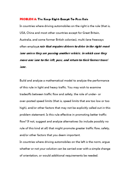
PROBLEM A: The Keep-Right-Except-To-Pass RuleIn countries where driving automobiles on the right is the rule (that is, USA, China and most other countries except for Great Britain, Australia, and some former British colonies), multi-lane freeways often employ a rule that requires drivers to drive in the right-most lane unless they are passing another vehicle, in which case they move one lane to the left, pass, and return to their former travel lane.Build and analyze a mathematical model to analyze the performance of this rule in light and heavy traffic. You may wish to examine tradeoffs between traffic flow and safety, the role of under- orover-posted speed limits (that is, speed limits that are too low or too high), and/or other factors that may not be explicitly called out in this problem statement. Is this rule effective in promoting better traffic flow? If not, suggest and analyze alternatives (to include possibly no rule of this kind at all) that might promote greater traffic flow, safety, and/or other factors that you deem important.In countries where driving automobiles on the left is the norm, argue whether or not your solution can be carried over with a simple change of orientation, or would additional requirements be needed.Lastly, the rule as stated above relies upon human judgment for compliance. If vehicle transportation on the same roadway was fully under the control of an intelligent system –either part of the road network or imbedded in the design of all vehicles using the roadway –to what extent would this change the results of your earlier analysis?PROBLEM B: College Coaching LegendsSports Illustrated, a magazine for sports enthusiasts, is looking for the “best all time college coach”male or female for the previous century. Build a mathematical model to choose the best college coach or coaches (past or present) from among either male or female coaches in such sports as college hockey or field hockey, football, baseball or softball, basketball, or soccer.Does it make a difference which time line horizon that you use in your analysis, i.e., does coaching in 1913 differ from coaching in 2013? Clearly articulate your metrics for assessment. Discuss how your model can be applied in general across both genders and all possible sports. Present your model’s top 5 coaches in each of 3 different sports.In addition to the MCM format and requirements, prepare a 1-2 page article for Sports Illustrated that explains your results and includes a non-technical explanation of your mathematical model that sports fans will understand.。

HIMCM 2014美国中学生数学建模竞赛试题Problem A: Unloading Commuter TrainsTrains arrive often at a central Station, the nexus for many commuter trains from suburbs of larger cities on a “commuter” line. Most trains are long (perhaps 10 or more cars long). The distance a passenger has to walk to exit the train area is quite long. Each train car has only two exits, one near each end so that the cars can carry as many people as possible. Each train car has a center aisle and there are two seats on one side and three seats on the other for each row of seats.To exit a typical station of interest, passengers must exit the car, and then make their way to a stairway to get to the next level to exit the station. Usually these trains are crowded so there is a “fan” of passengers from the train trying to get up the stairway. The stairway could accommodate two columns of people exiting to the top of the stairs.Most commuter train platforms have two tracks adjacent to the platform. In the worst case, if two fully occupied trains arrived at the same time, it might take a long time for all the passengers to get up to the main level of the station.Build a mathematical model to estimate the amount of time for a passenger to reach the street level of the station to exit the complex. Assume there are n cars to a train, each car has length d. The length of the platform is p, and the number of stairs in each staircase is q. Use your model to specifically optimize (minimize) the time traveled to reach street level to exit a station for the following:问题一:通勤列车的负载问题在中央车站,经常有许多的联系从大城市到郊区的通勤列车“通勤”线到达。

For office use onlyT1________________ T2________________ T3________________ T4________________ Team Control Number27820Problem ChosenBFor office use onlyF1________________F2________________F3________________F4________________ 2014Mathematical Contest in Modeling (MCM/ICM) Summary Sheet(Attach a copy of this page to your solution paper.)Research on Choosing the Best College Coaches Based on Data Envelopment AnalysisSummaryIn order to get the rank of coaches in differ ent sports and look for the ―best all time college coach‖ male or female for the previous century, in this paper, we build a comprehensive evaluation model for choosing the best college coaches based on data envelopment analysis. In the established model, we choose the length of coaching career, the number of participation in the NCAA Games, and the number of coaching session as the input indexes, and choose the victory ratio of games, the number of victory session and the number of equivalent champion as the output indexes. In addition, each coach is regarded as a decision making unit (DMU).First of all, with the example of basketball coaches, the relatively excellent basketball coaches are evaluated by the established model. By using LINGO software, the top 5 coaches are obtained as follows: Joe B. Hall, John Wooden, John Calipari, Adolph Rupp and Hank Iba.Secondly, the year 1938 is chosen as a time set apart to divide the time line into two parts. And then, basketball coaches are still taken as an example to evaluate the top 5 coaches used the constructed model in those two parts, respectively. The evaluated results are shown as: Doc Meanwell, Francis Schmidt, Ralph Jones, E.J. Mather, Harry Fisher before 1938, and Joe B. Hall, John Wooden, John Calipari, Adolph Rupp and Hank Iba after 1938. These results are accordant with those best coaches that were universally acknowledged by public. It suggests that the model is valid and effective. As a consequence, it can be applied in general across both genders and all possible sports.Thirdly, just the same as basketball coaches, football and field hockey coaches are also studied by using the model. After the calculation, the top 5 co aches of football’s results are as follows: Phillip Fulmer, Tom Osborne, Dan Devine, Bobby Bowden and Pat Dye, and field hockey’s are Fred Shero, Mike Babcock, Claude Julien, Joel Quenneville and Ken Hitchcock.Finally, although the top 5 coaches in each of 3 different sports have been chosen, the above-mentioned model failed to sort these coaches. Therefore, the super- efficiency DEA model is introduced to solve the problem. This model not only can evaluate the better coaches but also can rank them. As a result, we can choose the ―best all time college coach‖ from all the coaches easily.Type a summary of your results on this page. Do not includethe name of your school, advisor, or team members on this page.Research on Choosing the Best College Coaches Based on DataEnvelopment AnalysisSummaryI n order to get the rank of coaches in different sports and look for the ―best all time college coach‖ male or female for the previous century, in this paper, we build a comprehensive evaluation model for choosing the best college coaches based on data envelopment analysis. In the established model, we choose the length of coaching career, the number of participation in the NCAA Games, and the number of coaching session as the input indexes, and choose the victory ratio of games, the number of victory session and the number of equivalent champion as the output indexes. In addition, each coach is regarded as a decision making unit (DMU).First of all, with the example of basketball coaches, the relatively excellent basketball coaches are evaluated by the established model. By using LINGO software, the top 5 coaches are obtained as follows: Joe B. Hall, John Wooden, John Calipari, Adolph Rupp and Hank Iba.Secondly, the year 1938 is chosen as a time set apart to divide the time line into two parts. And then, basketball coaches are still taken as an example to evaluate the top 5 coaches used the constructed model in those two parts, respectively. The evaluated results are shown as: Doc Meanwell, Francis Schmidt, Ralph Jones, E.J. Mather, Harry Fisher before 1938, and Joe B. Hall, John Wooden, John Calipari, Adolph Rupp and Hank Iba after 1938. These results are accordant with those best coaches that were universally acknowledged by public. It suggests that the model is valid and effective. As a consequence, it can be applied in general across both genders and all possible sports.Thirdly, just the same as basketball coaches, football and field hockey coaches are also studied by using the model. After the calculation, the top 5 coaches of football’s results are as follows: Phillip Fulmer, Tom Osborne, Dan Devine, Bobby Bowden and Pat Dye, and field hockey’s are Fred Shero, Mike Babcock, Claude Julien, Joel Quenneville and Ken Hitchcock.Finally, although the top 5 coaches in each of 3 different sports have been chosen, the above-mentioned model failed to sort these coaches. Therefore, the super- efficiency DEA model is introduced to solve the problem. This model not only can evaluate the better coaches but also can rank them. As a result, we can choose the ―best all time college coach‖ from all the coaches easily.Key words: college coach；data envelopment analysis; decision making unit; comprehensive evaluationContents1. Introduction (4)2. The Description of Problem (4)3. Models (5)3.1Symbols and Definitions (5)3.2 GeneralAssumptions (6)3.3 Analysis of the Problem (6)3.4 The Foundation of Model (6)3.5 Solution and Result (8)3.6 sensitivity analysis (17)3.7 Analysis of the Result (19)3.8 Strength and Weakness (19)4.Improved Model............................................................................................................................ .. (20)4.1super- efficiency DEA model (20)4.2 Solution and Result (21)4.3Strength and Weakness (25)5. Conclusions (25)5.1 Conclusions of the problem...............................................................................,.25 5.2 Methods used in our models (26)5.3 Applications of our models (26)6.The article for Sports Illustrated (26)7.References (28)I. IntroductionAt present, the scientific evaluation index systems related to college coach abilities are limited, and the evaluation of coach abilities are mostly determined by the sports teams’game results, and it lacks of systematic, scientific and accurate evaluation with large subjectivity and one-sidedness, thus it can not objectively reflect the actual training level of coaches. In recent years, there appear many new performance evaluation methods, which mostly consider the integrity of the evaluation system. Thus they overcome a lot of weaknesses that purely based on the evaluation of game results. However, it is followed by the complexity of evaluation process and index system, as well as the great increase of the implementation cost. Data envelopment analysis is a non-parametric technique for evaluating the relative efficiency of a set of homogeneous decision-making units (DMUs) with multiple inputs and multiple outputs by using a ratio of the weighted sum of outputs to the weighted sum of inputs. Therefore, it not only simplifies the number of indexes, but also avoids the interference of subjective consciousness, thus makes the evaluation system more just and scientific.Based on the investigation and research of the US college basketball coach for the previous century, this paper aims at establishing a scientific and objective evaluation index system to assess their coaching abilities comprehensively. It provides reference for the relating sports management department to evaluate coaches and continuously optimize their coaching abilities. For this purpose, the DEA is successfully introduced into this article to establish a comprehensive evaluation model for choosing the best college coaches. It makes the assessment of the coaches in different time line horizon, different gender and different sports to testify the validity and the effectiveness of this approach.II. The Description of the Problem In order to find out the ―best all time college coach‖ for the previous century, a comprehensive evaluation model is needed to set up. Therefore, a set of scientific and objective evaluation index system should be established, which should meet the following principles or requirements:The principle of sufficiency and comprehensivenessThe index system should be sufficiently representative and comprehensivelycover the main contents of the coaches’ coaching abilities.The principle of independenceEach of the index should be clear and comparatively independent.The principle of operabilityThe data of index system comes from the existing statistics data, thus copying the unrealistic index system is not allowed.The principle of comparabilityThe comparative index should be used as far as possible to be convenientlycompared for each coach.After the establishment of evaluation index system, it requires the detailed model to make assessment and analysis for each coach. Currently, the comprehensive assessment is mostly widely used, but most of them need to be gave a weight. It is more subjective and not very scientific and objective. To avoid fixing the weight, the DEA method is adopted, which can figure out coaches’ rank eventually from the coach’s actual data.For the different time line horizon, the coaches’ rank is inevitably influenced by the team’s l evel and the sports, thus it requires discussion in different time line horizon to get the further results.Finally, the DEA model is applied to all coaches (either male or female) and all possible sports to get the rank, and then the model’s whole assessm ent basis and process should be explained to the readers in understandable words.III. Models3.1 Terms Definitions and Symbols Symbol ExplanationDMU k the k th DMU0DMU the target DMU, which is one of the nevaluated DMUs;ik x the i th input variable consumed0i x the i th input variable consumedjk y the j th output variable produced0j y the j th output variable produced1I The length of coaching career2I The number of taking part in NCAAtournament3I coaching session1Ovictory ratio of game3.2 General AssumptionsThe same level game difficulty in different regions and cities is equal for all teams.The value of the champion in different regions and cities is equal (without regard to team’s number in the region, the power and strength of the teams and other factors).The same game’s value is equal in different years (without regard to the team number in the year and other factors).The college’s level has no influence to the coach’s coaching performance.3.3 Analysis of the ProblemFor the current problem, first of all, a comprehensive evaluation model is needed to set up. Therefore, a set of scientific and objective evaluation index system should be established. The evaluation system of the coaches is comparatively mature, but it mainly based on the people’s subjective consciousness, thus the evaluation system we build requires more data to explain the problem, and it tries to assess each coach in a objective and just way without the interference of subjective factors.Secondly, the evaluation system we used is different due to the different games in different time periods. So the influence of different time periods to the evaluation results should be taken into account when we deal with the problem. Furthermore, it should be discussed in different cases.3.4 The Foundation of ModelData Envelopment Analysis (DEA), initially proposed by Charnes, Cooper and Rhodes [3], is a non-parametric technique for evaluating the relative efficiency of a set of homogeneous decision-making units (DMUs) with multiple inputs and multiple outputs by using a ratio of the weighted sum of outputs to the weighted sum of inputs. 2O the number of victory session3O The number of equivalent champion1Q the number of regular games champion2Q the number of league games champion3Qthe number of NCAA league gameschampionOne of the basic DEA models used to evaluate DMUs efficiency is the input-oriented CCR model, which was introduced by Charnes, Cooper and Rhodes [1]. Suppose that there are n comparatively homogenous DMUs (Here, we look upon each coach as a DMU), each of which consumes the same type of m inputs and produces the same type of s outputs. All inputs and outputs are assumed to be nonnegative, but at least one input and one output are positive.DMU k : the k th DMU, 1,2,,=k n ;0DMU : the target DMU, which is one of the n evaluated DMUs;ik x : the i th input variable consumed by DMU k , 1,2,,=i m ; 0i x : the i th input variable consumed by 0DMU , 1,2,,=i m ;jk y : the j th output variable produced by DMU k , 1,2,,=j s ;0j y : the j th output variable produced by 0DMU , 1,2,,=j s ; i u : the i th input weight, 1,2,,=i m ;In DEA model, the efficiency of 0DMU , which is one of the n DMUs, isobtained by using a ratio of the weighted sum of outputs to the weighted sum of inputs under the condition that the ratio of every entity is not larger than 1. The DEA model is formulated by using fractional programming as follows:()()000111112121,1,2,...,..,,,0,,,0max sr rj r m j i ij i sr rj r m i ij i T m T s j n s t v v v v u u u u y u hv x y u v x =====⎧⎪⎪≤=⎪⎪⎨⎪=≥⎪⎪=≥⎪⎩∑∑∑∑ （2）The above model is a fractional programming model, which is equivalent to the following linear programming model:00111010,1,2,...,..1,0,1,2,..;1,2,...,max s j r rj r sm i ij r rj r i m i ij i ir j n s t i m r sy h y w x w x w μμμ=====⎧-≤=⎪⎪⎪=⎨⎪⎪≥==⎪⎩∑∑∑∑ （3） Turned to another form is:101min ..0,1,2,,nj j j n j j j j x x s t j ny y θλθθλλ==⎧≤⎪⎪⎪⎪≥⎨⎪⎪≥=⎪⎪⎩∑∑无约束 3.5 Solution and Result3.5.1 Establishing the input and output index systemIn the DEA model, it requires defining a set of input index and a set of output index, and all the indexes should be the common data for each coach. Regarding the team as an unit, then the contribution that the coach made to the team can be regarded as input, while the achievement that the team made can be regarded as reward. In the following, we take the basketball coaches of NACC as an example to establish the input and output index system. These input indexes could be chosen as follows:1I :The length of coaching careerThe more game seasons a coach takes part in, the more abundant experience he has. This ki nd of coach’s achievement is easily affirmed by others. As the Figure 1 shows, the famous coach mostly experienced the long-time coaching career.Furthermore, the time the coach has contributed to the team is fundamental if they want to have a good result in the game. Thus the length of coaching career can be regarded as an index to evaluate the coach’s contribution to the team.Figure 1 The relationship between the length of coaching career and the number ofchampionsI: The number of taking part in NCAA tournament2Whether the coach takes the team to a higher level game has a direct influence on the team’s performance, and also it can reflect the coach’s coaching abilities, level and other factors.I: coaching session3For the reason of layers of elimination, the coaching session is not necessarily determined by the length of coaching career. It can be shown in the comparison between Figure 2 and Figure 3. Thus the number of coaching session can also be regarded as an index.Figure 2These output indexes could be chosen as follows:O: victory ratio of game1The index reflects the coach’s ability of command and control, and it a ttaches great importance to the evaluation of coach’s coaching abilities.O: the number of victory session2The case that the number of victory session reflected is different from that of victory ratio, only if get the enough number of victory session in a large number of coaching session, the acquired high victory ratio can reflect the coach’s high coaching level. If the victory occurs in a limited games, this kind of high victory ratio can not reflect the rules. It can be shown in the comparison between Figure 3 and Figure 4.Figure 3Figure 43O :The number of equivalent championThe honor that US college basketball teams acquired can be divided into three types: 1Q : the number of regular games champion; 2Q : the number of league games champion; 3Q : the number of NCAA league games champion. The threechampionship honor has different levels, and their importance is increasing in turn according to the reference. The weight 0.2、0.3、0.5 can be given respectively, and the number of equivalent champion can be figured out and used as an output index, as it shown in Table 1.5.0Q 3.0Q 2.0Q O 3213⨯+⨯+⨯=Table 1 Coach names Number of regular games champion (weight 0.2) Number of league games champion (weight 0.3) Number of NCAA league games championNumber of equivalent championAccording to Internet, the data of input and output are given by Table 2.Table 2(weight 0.5)Phog Allen 24 0 1 5.3 Fred Taylor 7 0 1 1.9 Hank Iba 15 0 2 4 Joe B. Hall 8 1 1 2.4 Billy Donovan 7 3 2 3.3 Steve Fisher 3 4 1 2.6 John Calipari 14 11 1 6.6 Tom Izzo 7 3 1 2.8 Nolan Richardso 9 6 1 3.9 John Wooden 16 0 10 8.2 Rick Pitino 9 11 2 6.1 Jerry Tarkanian 18 8 1 6.5 Adolph Rupp 28 13 4 11.5 John Thompson 7 6 1 3.7 Jim Calhoun 16 12 3 8.3 Denny Crum 15 11 2 7.3 Roy Williams 15 6 2 5.8 Dean Smith 17 13 2 8.3 Bob Knight 11 0 3 3.7 Lute Olson 13 4 1 4.3 Mike Krzyzewski 12 13 4 8.3 Jim Boeheim 11 5 1 4.2 Doc Meanwell 10 0 0 2 Ralph Jones 4 0 0 0.8 Francis Schmidt61.2Coach namesInput indexOutput index1I2I3I1O 2O3ONCAA tourament Thelength of coaching careerCoaching session Win-Lose %WinsNumber of equivalent championPhog Allen 4489780.735 719 5.3 Fred Taylor 5 18 455 0.653 297 1.9 Hank Iba84010850.6937524Since the opening of NACC tournament in 1938, thus the year 1938 is chosen as a time set apart. The finishing time point of coaching before 1938 is a period of time, while after 1938 is another period of time.For the time period before 1938, take the length of coaching career 1I , coaching session 3I as input indexes, and then take W-L %1O , victory session 2O , the number of regular games champion 1Q as output indexes. The results is shown in Table 3 after the data statistics of each index.For the time period after 1938, because they all take part in NACC, the input index and output index are just the same as that of all time period. The data statistics is just as shown in Table 3.Table 3Coach namesInput indexOutput index1I3I1O2O1QThe lengthof coachingcareerCoachingsessionW-L % WinsNumber of regular games championJoe B. Hall 10 16 463 0.721 334 2.4 Billy Donovan 13 20 658 0.714 470 3.3 Steve Fisher 13 24 739 0.658 486 2.6 John Calipari 14 22 756 0.774 585 6.6 Tom Izzo 16 19 639 0.717 458 2.8 Nolan Richardson 16 22 716 0.711 509 3.9 John Wooden 16 29 826 0.804 664 8.2 Rick Pitino 18 28 920 0.74 681 6.1 Jerry Tarkanian 18 30 963 0.79 761 6.5 Adolph Rupp 20 41 1066 0.822 876 11.5 John Thompson 20 27 835 0.714 596 3.7 Jim Calhoun 23 40 1259 0.697 877 8.3 Denny Crum 23 30 970 0.696 675 7.3 Roy Williams 23 26 902 0.793 715 5.8 Dean Smith 27 36 1133 0.776 879 8.3 Bob Knight 28 42 1273 0.706 899 3.7 Lute Olson 28 34 1061 0.731 776 4.3 Mike Krzyzewski 29 39 1277 0.764 975 8.3 Jim Boeheim303812560.759424.2Louis Cooke 27 380 0.654 248 5 Zora Clevenger 15 223 0.677 151 2 Harry Fisher 14 249 0.759 189 3 Ralph Jones 17 245 0.792 194 4 Doc Meanwell 22 381 0.735 280 10 Hugh McDermott 17 291 0.636 185 2 E.J. Mather 14 203 0.675 137 3 Craig Ruby 16 278 0.651 181 4 Francis Schmidt 17 330 0.782 258 6 Doc Stewart 15 291 0.663 193 2 James St. Clair162630.58215323.5.2 Solution and ResultIn this section, take Phog Allen as an example and make calculation as follows:Taking Phog Allen as 0DMU , then the input vector is 0x , the output vector is 0y , while the respective input and output weight vector are:From the Figure 2 it can be inferred thatT x )978,48,4(0= T y )3.5,719,735.0(0=After the calculation by LINGO then the efficiency value h 1 of DMU 1 is0.9999992.For other coaches, their efficiency value is figured out by the above calculation process as shown in Table 4.Table 4Coach namesInput indexOutput indexEfficiency value 1I2I3I1O 2O3ONCAA Tourna ment Thelength of coachin g careerCoachin g session W-L % Wins Number ofequivalent championJoe B. Hall 10 16 463 0.721 334 2.4 1John Wooden 16 29 826 0.804 664 8.2 1John Calipari 14 22 756 0.774 585 6.6 1Adolph Rupp 20 41 1066 0.822 876 11.5 1Hank Iba 8 40 1085 0.693 752 4 1Mike Krzyzewski 29 39 1277 0.764 975 8.3 1Roy Williams 23 26 902 0.793 715 5.8 1Jerry Tarkanian 18 30 963 0.79 761 6.5 0.9999997 Fred Taylor 5 18 455 0.653 297 1.9 0.9999996 Phog Allen 4 48 978 0.735 719 5.3 0.9999992 Tom Izzo 16 19 639 0.717 458 2.8 0.9785362 Dean Smith 27 36 1133 0.776 879 8.3 0.9678561 Jim Boeheim 30 38 1256 0.75 942 4.2 0.941031 Billy Donovan 13 20 658 0.714 470 3.3 0.9405422 Rick Pitino 18 28 920 0.74 681 6.1 0.9401934 Nolan Richardson 16 22 716 0.711 509 3.9 0.920282 Lute Olson 28 34 1061 0.731 776 4.3 0.9114966 John Thompson 20 27 835 0.714 596 3.7 0.8967647 Jim Calhoun 23 40 1259 0.697 877 8.3 0.8842854 Denny Crum 23 30 970 0.696 675 7.3 0.8823837 Bob Knight 28 42 1273 0.706 899 3.7 0.8769902 Steve Fisher 13 24 739 0.658 486 2.6 0.8543039For those coaches in the time period after 1938, the efficiency values, which is shown in Table 5, are figured out from the similar calculation process as Phog Allen.Table 5Coach namesInput index Output indexEfficiencyvalue 1I3I1O2O1QThelengthofcoaching careerCoaching sessionW-L % WinsNumberof regularchampionDoc Meanwell 22 381 0.735 280 10 1Francis Schmidt 17 330 0.782 258 6 1Ralph Jones 17 245 0.792 194 4 1E.J. Mather 14 203 0.675 137 3 0.9999999Harry Fisher 14 249 0.759 189 3 0.999999 Zora Clevenger 15 223 0.677 151 2 0.9328517 Doc Stewart 15 291 0.663 193 2 0.8910155 Craig Ruby 16 278 0.651 181 4 0.859112 Louis Cooke 27 380 0.654 248 5 0.8241993 Hugh McDermott 17 291 0.636 185 2 0.8091489 James St. Clair 16 263 0.582 153 2 0.7468237Choose basketball, football and field hockey and make calculationsThe calculation result statistics of basketball is shown in Table 4.The calculation result statistics of football is shown in Table 6.Table 6Coach NamesInput index Output indexEfficiencyvalue Total ofthe BowlThelength ofcoachingcareerCoachingsessionW-L % WinsNumberofchampionPhillip Fulmer 15 17 204 0.743 151 8 1 Tom Osborne 25 25 307 0.836 255 12 1 Dan Devine 10 22 238 0.742 172 7 1 Bobby Bowden 33 40 485 0.74 357 22 1 Pat Dye 10 19 220 0.707 153 7 1 Bobby Dodd 13 22 237 0.713 165 9 1Bo Schembechler 17 27 307 0.775 234 5 1 Woody Hayes 11 28 276 0.761 205 5 1.000001 Joe Paterno 37 46 548 0.749 409 24 1 Nick Saban 14 18 228 0.748 170 8 0.9999993 Darrell Royal 16 23 249 0.749 184 8 0.9653375 John Vaught 18 25 263 0.745 190 10 0.9648578 Steve Spurrier 19 24 300 0.733 219 9 0.9639218 Bear Bryant 29 38 425 0.78 323 15 0.9623039 LaVell Edwards 22 29 361 0.716 257 7 0.9493463 Terry Donahue 13 20 233 0.665 151 8 0.9485608 John Cooper 14 24 282 0.691 192 5 0.94494 Mack Brown 21 29 356 0.67 238 13 0.9399592 Bill Snyder 15 22 269 0.664 178 7 0.9028372 Ken Hatfield 10 27 312 0.545 168 4 0.9014634 Fisher DeBerry 12 23 279 0.608 169 6 0.9008829 Don James 15 22 257 0.687 175 10 0.8961777Bill Mallory 10 27 301 0.561 167 4 0.8960976 Ralph Jordan 12 25 265 0.674 175 5 0.8906943 Frank Beamer 21 27 335 0.672 224 9 0.8827047 Don Nehlen 13 30 338 0.609 202 4 0.8804766 Vince Dooley 20 25 288 0.715 201 8 0.8744984 Jerry Claiborne 11 28 309 0.592 179 3 0.8731701 Lou Holtz 22 33 388 0.651 249 12 0.8682463 Bill Dooley 10 26 293 0.558 161 3 0.8639017 Jackie Sherrill 14 26 304 0.595 179 8 0.8435327 Bill Yeoman 11 25 276 0.594 160 6 0.8328854 George Welsh 15 28 325 0.588 189 5 0.820513 Johnny Majors 16 29 332 0.572 185 9 0.807564 Hayden Fry 17 37 420 0.56 230 7 0.792591The calculation result statistics of field hockey is shown in Table 7.Table 7Coach namesInput index Output indexEfficiencyvalue Total ofthe BowlThelength ofcoachingcareerCoachingsessionW-L % WinsNumberofchampionFred Shero 110 10 734 0.612 390 2 1 Mike Babcock 131 11 842 0.63 470 1 1 Claude Julien 97 11 749 0.61 411 1 1 Joel Quenneville 163 17 1270 0.617 695 2 1 Ken Hitchcock 136 17 1213 0.602 642 1 1 Marc Crawford 83 15 1151 0.556 549 1 0.9999998 Scotty Bowman 353 30 2141 0.657 1244 9 0.9999996 Hap Day 80 10 546 0.549 259 5 0.9999995 Toe Blake 119 13 914 0.634 500 8 0.9999994 Eddie Gerard 21 11 421 0.486 174 1 0.999999 Art Ross 65 18 758 0.545 368 1 0.9854793 Peter Laviolette 82 12 759 0.57 389 1 0.9832692 Bob Hartley 84 11 754 0.56 369 1 0.9725678 Jacques Lemaire 117 17 1262 0.563 617 1 0.9706553 Glen Sather 127 13 932 0.602 497 4 0.9671556 John Tortorella 89 14 912 0.541 437 1 0.9415468 John Muckler 67 10 648 0.493 276 1 0.9379403 Lester Patrick 65 13 604 0.554 281 2 0.9246999 Mike Keenan 173 20 1386 0.551 672 1 0.8921282 Al Arbour 209 23 1607 0.564 782 4 0.8868355 Frank Boucher 27 11 527 0.422 181 1 0.8860263Pat Burns 149 14 1019 0.573 501 1 0.8803399 Punch Imlach 92 14 889 0.537 402 4 0.8795251Darryl Sutter 139 14 1015 0.559 491 1 0.8754745Dick Irvin 190 27 1449 0.557 692 4 0.8688287Jack Adams 105 20 964 0.512 413 3 0.8202896 Jacques Demers 98 14 1007 0.471 409 1 0.7982191 3.6 sensitivity analysisWhen determining the number of equivalent champion, the weight coefficient is artificially determined. During this process, different people has different confirming method.Consequently, we should consider that when the weight coefficient changes in a certain range, what would happen for the evaluation result?For the next step, we will take the basketball coaches as example to illustrate the above-mentioned case.The weight coefficient changes is given by Table 12. The changes of evaluation results is shown in Table 13.Table 12Coach names Number ofregulargameschampion(weight0.2)Number ofleaguegameschampion(weight 0.4)Number ofNCAA leaguegameschampion(weight0.4)Number ofequivalentchampionPhog Allen 24 0 1 5.2 Fred Taylor 7 0 1 1.8 Hank Iba 15 0 2 3.8 Joe B. Hall 8 1 1 2.4 Billy Donovan 7 3 2 3.4 Steve Fisher 3 4 1 2.9 John Calipari 14 11 1 7.6 Tom Izzo 7 3 1 3 NolanRichardso9 6 1 4.4 John Wooden 16 0 10 7.2 Rick Pitino 9 11 2 7 JerryTarkanian18 8 1 7.2 Adolph Rupp 28 13 4 12.4 JohnThompson7 6 1 4.2 Jim Calhoun 16 12 3 9.2 Denny Crum 15 11 2 8.2 Roy Williams 15 6 2 6.2Dean Smith 17 13 2 9.4 Bob Knight 11 0 3 3.4 Lute Olson 13 4 1 4.6 MikeKrzyzewski12 13 4 9.2 Jim Boeheim 11 5 1 4.6Table 13Coach namesI nput index O utput indexEfficiencyvalue 1I2I3I1O2O3ONCAATournamentThelength ofcoachingCareerCoachingsessionW-L %WinsNumber ofequivalentchampionJohn Wooden 16 29 826 0.804 664 7.2 1.395729 John Calipari 14 22 756 0.774 585 7.6 1.318495 Joe B. Hall 10 16 463 0.721 334 2.4 1.220644 Adolph Rupp 20 41 1066 0.822 876 12.4 1.157105Hank Iba 8 40 1085 0.693 752 3.8 1.078677 Roy Williams 23 26 902 0.793 715 6.2 1.034188 Fred Taylor 5 18 455 0.653 297 1.8 1.013679 Jerry Tarkanian 18 30 963 0.79 761 7.2 1.007097 Phog Allen 4 48 978 0.735 719 5.2 0.999999 Jim Boeheim 30 38 1256 0.75 942 4.6 0.984568Tom Izzo 16 19 639 0.717 458 3 0.978536 Dean Smith 27 36 1133 0.776 879 9.4 0.96963Mike Krzyzewski 29 39 1277 0.764 975 9.2 0.960445 Rick Pitino 18 28 920 0.74 681 7 0.940614 Billy Donovan 13 20 658 0.714 470 3.4 0.940542 Nolan Richardson 16 22 716 0.711 509 4.4 0.920282 Lute Olson 28 34 1061 0.731 776 4.6 0.911496 John Thompson 20 27 835 0.714 596 4.2 0.896765 Jim Calhoun 23 40 1259 0.697 877 9.2 0.884227 Denny Crum 23 30 970 0.696 675 8.2 0.882805 Bob Knight 28 42 1273 0.706 899 3.4 0.87699 Steve Fisher 13 24 739 0.658 486 2.9 0.854304From the Table 13, it can been seen that the top 5 coaches are: John Wooden, John Calipari, Joe B. Hall, Adolph Rupp, Hank Iba. The result is in accordance with。

2014 MCM ProblemsPROBLEM A: The Keep-Right-Except-To-Pass RuleIn countries where driving automobiles on the right is the rule (that is, USA, China and most other countries except for Great Britain, Australia, and some former British colonies), multi-lane freeways often employ a rule that requires drivers to drive in the right-most lane unless they are passing another vehicle, in which case they move one lane to the left, pass, and return to their former travel lane.在一些以行车靠右为规则的国家中（比如美国、中国以及除了大不列颠、澳大利亚和一些前英属殖民国家以外的其他国家），多行道的高速公路经常采用要求驾驶人在除超车以外时都靠右行驶的交通规则。

Build and analyze a mathematical model to analyze the performance of this rule in light and heavy traffic. You may wish to examine tradeoffs between traffic flow and safety, the role of under- or over-posted speed limits (that is, speed limits that are too low or too high), and/or other factors that may not be explicitly called out in this problem statement. Is this rule effective in promoting better traffic flow? If not, suggest and analyze alternatives (to include possibly no rule of this kind at all) that might promote greater traffic flow, safety, and/or other factors that you deem important.1、请你建立和分析一个数学模型来分析这个规则在交通畅通和交通堵塞条件下的表现。

PROBLEM A： The Keep—Right-Except-To-Pass Rule靠右除了超车规则In countries where driving automobiles on the right is the rule （that is， USA， China and most other countries except for Great Britain， Australia， and some former British colonies）， multi—lane freeways often employ a rule that requires drivers to drive in the right-most lane unless they are passing another vehicle， in which case they move one lane to the left， pass， and return to their former travel lane。

在一些开车靠右行驶的国家(美国,中国和大多数的其他国家，除了英国,澳大利亚和一些英国的殖民地），多车道高速公路通常采用一个规则，要求司机在大多数高速公路上开车时靠右行驶，除非他们在超车时，这种情况下，他们要移到左边的车道,超车然后回到他们从前的车道。

Build and analyze a mathematical model to analyze the performance of this rule in light and heavy traffic. You may wish to examine tradeoffs between traffic flow and safety，the role of under- or over-posted speed limits (that is， speed limits that are too low or too high）, and/or other factors that may not be explicitly called out in this problem statement。

1985 年美国大学生数学建模竞赛MCM 试题1985年MCM:动物种群选择合适的鱼类和哺乳动物数据准确模型。

模型动物的自然表达人口水平与环境相互作用的不同群体的环境的重要参数,然后调整账户获取表单模型符合实际的动物提取的方法。

包括任何食物或限制以外的空间限制,得到数据的支持。

考虑所涉及的各种数量的价值,收获数量和人口规模本身,为了设计一个数字量代表的整体价值收获。

找到一个收集政策的人口规模和时间优化的价值收获在很长一段时间。

检查政策优化价值在现实的环境条件。

1985年MCM B:战略储备管理钴、不产生在美国,许多行业至关重要。

(国防占17%的钴生产。

1979年)钴大部分来自非洲中部,一个政治上不稳定的地区。

1946年的战略和关键材料储备法案需要钴储备,将美国政府通过一项为期三年的战争。

建立了库存在1950年代,出售大部分在1970年代初,然后决定在1970年代末建立起来,与8540万磅。

大约一半的库存目标的储备已经在1982年收购了。

建立一个数学模型来管理储备的战略金属钴。

你需要考虑这样的问题:库存应该有多大?以什么速度应该被收购?一个合理的代价是什么金属?你也要考虑这样的问题:什么时候库存应该画下来吗?以什么速度应该是画下来吗?在金属价格是合理出售什么?它应该如何分配?有用的信息在钴政府计划在2500万年需要2500万磅的钴。

美国大约有1亿磅的钴矿床。

生产变得经济可行当价格达到22美元/磅(如发生在1981年)。

要花四年滚动操作,和thsn六百万英镑每年可以生产。

1980年,120万磅的钴回收,总消费的7%。

1986 年美国大学生数学建模竞赛MCM 试题1986年MCM A:水文数据下表给出了Z的水深度尺表面点的直角坐标X,Y在码(14数据点表省略)。

深度测量在退潮。

你的船有一个五英尺的草案。

你应该避免什么地区内的矩形(75200)X(-50、150)?1986年MCM B:Emergency-Facilities位置迄今为止,力拓的乡牧场没有自己的应急设施。

For office use onlyT1________________ T2________________ T3________________ T4________________Team Control Number27400Problem ChosenAFor office use onlyF1________________F2________________F3________________F4________________2014 Mathematical Contest in Modeling (MCM) Summary Sheet(Attach a copy of this page to your solution paper.)Type a summary of your results on this page. Do not includethe name of your school, advisor, or team members on this page.SummaryThe aim of this paper is to evaluate the performance of the changing lane rule named Keep-Right-Except-To-Pass and compare other rules we’ve constructed with the given one. The performance of changing lane rules mainly manifest in safety and traffic flow. Meanwhile, safety is influenced by posted speed limits and traffic density and traffic flow is influenced by average speed.First we construct Model 1 to describe the relationship between posted speed limits, traffic density and safety, noting that safety has negative correlation with collision times and can be fully expressed by it. Therefore we use Matlab to imitate the changing lane and collision process. Then we construct Model 2 to describe the relationship between traffic flow and average speed. Combining the result of Model 1and 2, we can conclude that the higher the posted speed limits and the lower the traffic density, the higher level safety an traffic flow could reach, and the Keep-To-Right-Except-To-Pass rule has the best performance.Then we construct Model 3 to compare some normal changing lane rules with the given one and with each other. Thus we imitate all the rules using algorithm given by model 1. We introduce a new concept named Standard Time to express traffic flow and still collision times to express safety. The result is that when a freeway road contains 2 lanes, the given rule shows the best performance. And when the number of lanes becomes 3, then the Choose-Speed rule, a very common traffic rule acts the best.As for the left-driving countries, we first choose the best rules and mirror symmetrically modify them. Then use the method of Model 2 to imitate performances of these rules. We have observed that these two best rules can be simply carried over.Finally, we have a short discussion about the intelligent system. Since speed can be fastest and changing lanes can be well planned, we regard this system as absolutely safe traffic which has the largest traffic flow.Team #27400 Page 1 of 161.Introduction1.1 Analysis to the problemThis problem can be divided into 4 requirements that we must meet, listed as follows:(1)Build a mathematical model to demonstrate the essence of Keep-Right-Except-To-Pass rule in light and heavy traffic;(2)Show the effects of other reasonable changing-lane rules or conditions by using themodified model built in the former requirement;(3)Determine whether the left-side-driving countries can use the same rule(s) withsimple mirror symmetric modification, or must add some requirements to guaranteethe safety or traffic flow;(4)Construct an intelligent traffic system which does not depend on humans’ compliance,and then compare the effects with earlier analysis.Therefore, this problem requires us to evaluate the performances of several changing-lane rules, especially the Keep-Right-Except-To-Pass rule while performances mainly manifest in traffic flow and safety. It is obvious that speed limit and the number of cars influent cars’ speed and then the performances of those rules.To solve requirement (2), we will use the same method as above. But all rules weconstructed should be discussed, imitated and compare with each other.To discuss the left-driving countries, we will conclude the best rules from requirement2 and apply to those countries. Then compare results with that of right-driving countries.If the results are totally the same, then those rules can be simply carried over with simple change. If not, additional requirement are needed.As for the intelligent system, we assume no collision will happen. So a simplediscussion is feasible.1.2 Crucial method for the problemTo imitate the process of changing lanes and collision, we will construct an algorithm named Changing-line and Collision. This will show the state of a number of car on the same stretch of freeway road, including going straight, changing lane to pass and traffic collision. The imitation process will be delivered on Matlab;2.Symbols and definitionSymbol Definition UnitσStandard Deviation of Speed miles/hmiles/hV85% Percentile of Normal85Distributionmiles/hV70% Percentile of Normal70DistributionDENS Traffic Density (Note: expressed by thenumber of cars) ST Standard Time \FLO Traffic Flow \CT Collision Times \3.General hypotheses for all models(1) All freeway roads contain either two or three lanes.(2) Overtaking Principle: the latter car must change lane and overtake the car right in front it if its speed is faster.(3) No violation of the rules.(4) The intelligent traffic system has no collision.(5) Road indicates one direction of the road.(6) Each cars remains constant speed no matter it goes straight or change lane.(7) Changing lane doesn’t cost time.(8) Given a traffic density, the average speed of cars is constant.(9) All discussions are confined to one stretch of road that is long enough to allow a series of cars to go across.4.Model establishment4.1 PreparationFirst, we must discuss what “changing-lane” is. For a two-lane road, if one car is going to change its lane to the left, then the right side lane “loses” one car and the left side lane “acquires” one, and vice versa. If the road contains three lanes, we can regard it as two “two-lane road”. This property also holds for an n-lane (n>2) road, which means we could regard it as (n-1) two-lane road. Therefore, changing-lane is the relation between two lanes. We just need to analyze a two-lane road to uncover the principle of changing lane and collision.Second, influence relationship figures are given below. In these figures, factors at lower level influence those at upper level. Safety will be expressed by collision times( ).Figure 1. General influence relationshipThird, we have constructed three additional changing-lane rules and shall describe these five rules in mathematical language. The original Keep-Right-Except-To-Pass rule is denoted Rule 1.Rule 1: Keep-Right-Except-To-Pass. If A B v v >, then car A goes left, overtakes car B and then gets back to the right lane.Figure 2. Rule one: Keep-Right-Except-To-PassRule 2: Free-Overtaking. If A B v v > and A C v v >, then car A changes lane to the left, passing B, and then to the right, passing C. And if there still exists a car D in front of A and A D v v >, car A will change to the left lane, pass D and then go straight. The following figure shows the case when the number of lanes is two, and it is identical for the case of 3 lanes.Figure 3. Rule 2: Free-OvertakingRule 3: Pass-Left. For a three-lane freeway road, if B A C v v v >>, then car A changes to the middle lane, and car B to the left lane, and finally they should get back to their original lane.Figure 4. Rule 3: Pass-LeftRule 4: Choose-Speed. Each lane of the road has a posted speed limit interval. We denote the left lane fast lane, right one slow lane and the middle one mid-lane. Drivers should choose lane according to their cars ’ speed.4.2 Model 1: Changing Lane and Collision Algorithm 4.2.1 Flow Diagram*To check Matlab code, please refer to Appendix 1. Note: we only use collision times to express safety.Figure 5. Flow Diagram of the Changing Lane and Collision Algorithm Comments:(1) The 1000*2 matrix stands for a stretch freeway road that contains two lanes;(2) Speed of cars is a series of random numbers which stands for the units they are to go forward each time;(3) Cars enter the road from the right lane.(4) If two cars collide, their speed will become zero but will not affect other cars. Accordingly, the position of collision will be valuated zero.To show how this algorithm works, we now give an example of a road, length 7 and five carswith different speed:Figure 6. An Example of the Algorithm4.2.2 Relationship between Average Speed, Standard Deviation of Speed and Posted Speed LimitsWe have mentioned in the last section that the speed of cars obeys normal distribution [3]. Now we deduce the relationship between ,μσ and PSL .Figure 7. Speed of cars obey normal distributionWe know from reference [4](page 15) that:857.6570.98V PSL =+⋅①The above foemula can be applied to all types of roads. Equation ② from reference [5](page 53):70-6.541+2.4V σ=⋅②Referring to the table of standard normal distribution, we have70V μσ-=0.52③ 85V μσ-=1.04④Considering formula ②③, we have=1.88-6.541μσ⑤Considering formula ①④, we have7.657+0.98=1.04PSL μσ-⑥Considering formula ⑤⑥, we have14.198+0.98=2.92PSLσ⑦0.98*=13.6012PSL μ-⑧Formula ⑦⑧ explains that the higher the posted speed limits, the greater the variance of speed and same to the average speed.0.9813.6012MU PSL =-⑨4.2.3 Process of ImitationWe now use control-variable method to describe the impact of traffic density and posted speed limits on safety. Therefore, we consider:(1) Traffic density being constant, the impact of variation of posted speed limits on safety; (2) Posted speed limits being constant, the impact of variation of traffic density on safety.When traffic density is constant:Table 1.Variation of Posted Speed LimitsPSL 50 60 70 80 90 100 μ 34.1481 40.4577 46.7673 53.0769 59.3865 65.6961 σ21.6432 24.9993 28.3555 31.7116 35.0678 38.424Figure 8. Variation of μ and σ along with Variation of PSLNote: SIGMA=σ, MU=μWhen posted speed limits is constant:Table 2.Variation of the number of carsThe number of cars 5 10 20 30 40 50Therefore we will acquire 6*6 groups of data when PSL is constant and 6*6 groups of data when traffic density is constant.4.3 Model 2: Relationship between Traffic Flow and Average SpeedIt is obvious that traffic flow is the function of average.We denote:=⋅+>FLO k MU c k(0)4.4 Model 3: Rules and Performances4.4.1 AnalysisIn section 4.1 we have listed four changing lane rules. Now we need to compare their effect and evaluate which rule has the best performance.According to the establishment of model 1, performances are fully expressed by safety and traffic flow, and safety has negative correlation with collision times. We can acquire the related data by imitation like model 1. However, since rules have changed, average speed of the road under different rules is different and is merely decided by PSL.Thus we introduce a new concept, namely, Standard Time(ST). Definition: time cost by each move of cars is called standard time. With this concept, we don’t need to calculate the real time cost by cars when going across a stretch of road, but count how many moves cars should make. Standard time has positive correlation with traffic flow, and we can denote:ST k FLO k=⋅>(0)4.4.2 Imitation ProcessConstruct a matrix. If the road contains two lanes, then the matrix size is 150*2; if it contains three lanes, then the size is 150*3. Arrange 40 random positions for each column vectors, and the numbers, as described before, obey normal distribution. Let other variables be constant, we discuss the impact of different rules on safety and traffic flow.Operations are as follows:(1) Distribute a series positions(40 for each column vector as described) for the matrix.(2) Valuate each position a number that obey normal distribution.(3) Apply one of the rules to the matrix. Those numbers will either “collide ” or “keep moving ” until all the position are valuated zero. (4) Record collision times and the spent standard time.(5) Apply another rule to the matrix, repeat steps (1) through (4).Statistically analyzing the data acquired and comparing the performances of different rules, we can decide advantages and disadvantages of each rule.4.4.3 Use the Method of 4.4.2 to Estimate Left-driving CountriesWe will conclude the best two rules and then apply the methods in section 4.4.2 to the left-driving country and estimate the performance of the two rules. Operation steps:(1) Mirror symmetrically modify the chosen rules; (2) Refer to the steps in section 4.4.2; (3) Compare with the results in 4.4.2.5. Model solution5.1 Model 1During the imitation process, we do the experiment for times for each case and then analyze all the results. We will show part of our statistical data. To view full data, please refer to Appendix 2.(1) Given DENS=30, the result is as follows:Table 3.Relationship between Changing Lane Times, Collision Times and PSL when DENS=30PSL Changing-lane times Average Collision TimesAverag-Line chart:Figure 9. Variation of Changing Lane Times and Collision Times along with Variation ofPSL(2) Given PSL=70, the result is as follows:Table 4.Relationship between Changing Lane Times, Collision Times and Number of Times whenPSL=70NumberChanging Lane Times Average Collision Time Average Line chart:Figure 10. Variation of Changing Lane Times and Collision Times along with Variation ofnumber of cars5.2 Model 2We know from formula ⑨, section 4.2.2 that0.9813.6012MU PSL =-Considering formula ⑨ and formula in 4.3, we have:0.9813.6012FLO k PSL k c =⋅-+5.3 Model 3The result of section 4.4.2 is given below:Table 5.Collision Times and Standard Time of each ruleRule →Rule 1 Rule 2(2Rule 3 Rule 2(3 Rule 4Extract the row of Average ST and Average CTTable 6.Average Collision Times and Average Standard Time of each rule The result of 4.4.3 is given below:Table 7.Collision Times and Standard Time of Rule 1 and Rule 4 Applied to Left-driving Countries6.Conclusion6.1 Conclusion of model 1 and 2We can conclude from model 1 that safety will decrease along with the growth oftraffic density. Safety will also decrease while the posted speed limits(PSL) is raised.However, comparing to PSL, traffic density has greater impact on safety while PSL can hardly influence safety.From model 2, we can conclude that traffic flow has liner growth along with the raise of PSL.The following table has summed up model 1 and 2.Table . 8Evaluation of Rule Performances in Different Road conditions6.2 Conclusion of model 3We can know from table 6 that when the number of lanes is 2, rule 1 is not very different from rule 2 in terms of traffic flow but is much safer than rule 2. When the number of lanes is 3, rule 3 is safest rule, but rule 4 will become both safe and efficient. Meanwhile, Free-Overtaking rule, actually meaning no rule, is most dangerous. Therefore, we have chosen rule 1 and rule 4 as the best rules.Result of section 4.4.3 is showed below. Note that original rules are listed on the left and modified on the right.Table .9Comparison between the Modified Rules and the OriginalFrom the table above, we can conclude that no difference between left-driving and right-driving countries. Therefore, those rules can be simply carried over with simple mirror symmetric modification.6.2 Conclusion of intelligent systemSince all the cars are controlled by a high-tech computer, we assume this system will never have an accident until the computer crashes. So every car reach their fastest speed, the order of overtaking can be calculated to avoid collision. Therefore, safety and traffic flow reach the highest level.7. References[1] Mark M. Meerschaert. Mathematical Modelling (Third Edition). Beijing: China Machine Press, 2008.12[2] Solomon. Accidents on Main Rural Highways Re la ted to Speed, Driver, and Vehicle[R]. Washing ton D. C: Federal Highway Administration, 1964[3] Lu Jian, Sun Xinglong, Daiyue. Regression analysis on speed distribution characteristics of ordinary road. Nanjing: Journal of Southeast University(Natural Science Edition), 2012.2 (in Chinese).[4] Wang Lijin. Research on Speed Limits and Operating Speed for Freeway. Beijing: Beijing University of Technology, 2011.5 (in Chinese).8. AppendixAppendix 1. Matlab Codeclear;clc;highway=zeros(1000,2);%define road%crash_times = 0;%define collition times%change_lane_times=0;%define change lane times%num_of_car=5; %definedefine number of car%MU=84.3898;SIGMA=20.4406;randspe=[];j=1;while j<=num_of_carx=round(normrnd(MU,SIGMA,1,1));if x>0randspe(j,1)=x; %define speed and gualentee %j=j+1;endx=0;endrandpla=[];for i=1:num_of_carx=ceil(rand(1)*1000);if find(randpla==x)x=ceil(rand(1)*1000); %define location and guarantee the car located in different place%endrandpla(i,1)=x;endfor i=1:num_of_carhighway(randpla(i,1),2)=randspe(i,1); %insert every car in different speed at diferent place %speed(i,1)=0;pla(i,1)=0;endinitialr_highway=highway; %record intialr-highway statement%disp(initialr_highway)disp('Aboveis the stateof initialr highway')while sum(sum(highway))~=0i=1;speed(1)=0; pla(1)=0;for j=1:length(highway) %Store the location and speed of each carif highway(j,2)~=0 ....to pla_matrix and speed_matrix separately%speed(i)=highway(j,2);pla(i)=j;i=i+1;endendcount=length(pla);while count>1 %When the differerce of two adjacent car's speed is greater than their distance,thenif speed(count)-speed(count-1)>=abs(pla(count)-pla(count-1)) ... the later car must change lane to the left% highway(pla(count),1)=highway(pla(count),2);highway(pla(count),2)=0;change_lane_times=change_lane_times+1;endcount=count-1;endlane_changed= highway; %record lane_changed highway statement%disp(lane_changed)disp('Aboveis the state of after-changed lane highway ')k=1;pas_spe(1)=0;pas_pla(1)=0;for j=1:length(highway)if highway(j,1)~=0pas_spe(k)=highway(j,1);pas_pla(k)=j;k=k+1;endendcount=length(pas_pla); %delete crashed car%while count>1if pas_spe(count)-pas_spe(count-1)>=abs(pas_pla(count)-pas_pla(count-1))highway(pas_pla(count),1)=0;highway(pas_pla(count-1),1)=0;crash_times=crash_times+1;endcount=count-1;endaft_adjust = highway;disp(aft_adjust)disp('Above is after adjusted highway')for i=1:length(highway)for j=1:2if i-highway(i,j)>0highway(i-highway(i,j),j)=highway(i,j);%move forward%endhighway(i,j)=0;endendfor i=1:length(highway)if highway(i,1)~=0&&highway(i,2)==0%back to right%highway(i,2)=highway(i,1);highway(i,1)=0;endendback_to_right = highway; %record lane_changed highway statement%disp(back_to_right);disp('Aboveis the state of back_to_right lane highway.');pla=0;speed=0;pas_pla=0;pas_spe=0;endfprintf('change_lane_time ','\n');disp(change_lane_times)fprintf('crash_time ','\n');disp(crash_times)Appendix 2. Data of ImitationPSL Change lane times Mean Crash times MeanNumberof cars=5 50 2 2 2 2.0 0 0 0 0.0 60 3 2 3 2.7 0 0 0 0.0 70 1 0 1 0.7 0 0 0 0.0 80 2 0 1 1.0 0 0 0 0.0 90 0 0 3 1.0 0 0 0 0.0 100 1 3 2 2.0 0 0 0 0.0Numberof 50 7 5 11 7.7 0 0 0 0.0 60 8 11 8 9.0 0 1 0 0.3cars=10 70 10 6 7 7.7 1 0 1 0.780 6 7 10 7.7 0 1 1 0.790 4 7 4 5.0 1 2 0 1.0100 6 3 3 4.0 1 1 1 1.0Numberof cars=20 50 47 29 38 38.0 1 2 2 1.7 60 30 34 20 28.0 2 0 1 1.0 70 15 17 22 18.0 0 2 3 1.7 80 18 22 16 18.7 0 2 1 1.0 90 20 10 22 17.3 1 1 2 1.3 100 21 15 13 16.3 2 2 1 1.7Numberof cars=30 50 61 60 48 56.3 5 4 2 3.7 60 46 42 45 44.3 4 1 2 2.3 70 42 38 48 42.7 4 5 3 4.0 80 43 32 47 40.7 2 5 5 4.0 90 32 41 33 35.3 3 4 5 4.0 100 26 27 24 25.7 2 2 4 2.7Numberof cars=40 50 65 100 74 79.7 8 4 8 6.7 60 56 77 75 69.3 5 8 3 5.3 70 53 64 62 59.7 4 5 5 4.7 80 52 60 60 57.3 3 7 3 4.3 90 44 53 48 48.3 5 4 4 4.3 100 43 50 38 43.7 1 7 0 2.7Numberof cars=50 50 82 86 106 91.3 12 12 10 11.3 60 80 68 72 73.3 10 9 13 10.7 70 82 75 81 79.3 8 7 10 8.3 80 61 72 58 63.7 9 7 11 9.0 90 57 54 54 55.0 6 7 11 8.0 100 64 50 51 55.0 7 9 8 8.0PSL=705 1 0 1 0.7 0 0 0 0.0 10 1067 7.7 1 0 1 0.7 20 15 17 22 18.0 0 2 3 1.7 30 42 38 48 42.7 4 5 3 4.0 40 53 64 62 59.7 4 5 5 4.7 50 82 75 81 79.3 8 7 10 8.3PSL Change lanetimescollisiontimesDensityChange lanetimescollisiontimes50 56.33333333 3.666666667 5.0 0.666666667 060 44.33333333 2.333333333 10.0 7.666666667 0.666666667 70 42.66666667 4 20.0 18 1.666666667 80 40.66666667 4 30.0 42.66666667 490 35.33333333 4 40.0 59.66666667 4.666666667 100 25.66666667 2.666666667 50.0 79.33333333 8.333333333。

2010 MCM ProblemsPROBLEM A: The Sweet SpotExplain the “sweet spot” on a baseball bat.Every hitter knows that there is a spot on the fat part of a baseball bat where maximum power is transferred to the ball when hit. Why isn’t this spot at the end of the bat? A simple explanation based on torque might seem to identify the end of the bat as the sweet spot, but this is known to be empirically incorrect. Develop a model that helps explain this empirical finding.Some players believe that “corking” a bat (hollowing out a cylinder in the head of the bat and filling it with cork or rubber, then replacing a wood cap) enhances the “sweet spot” effect. Augment your model to confirm or deny this effect. Does this explain why Major League Baseball prohibits “corking”?Does the material out of which the bat is constructed matter? That is, does this model predict different behavior for wood (usually ash) or metal (usually aluminum) bats? Is this why Major League Baseball prohibits metal bats?MCM 2010 A题：解释棒球棒上的“最佳击球点”每一个棒球手都知道在棒球棒比较粗的部分有一个击球点，这里可以把打击球的力量最大程度地转移到球上。

85-09历年美赛（MCM）中文试题校苑资源网整理历年美国大学生数学建模赛题目录MCM85问题-A 动物群体的管理.............................................................................................- 3 - MCM85问题-B 战购物资储备的管理.....................................................................................- 3 - MCM86问题-A 水道测量数据.................................................................................................- 4 - MCM86问题-B 应急设施的位置.............................................................................................- 4 - MCM87问题-A 盐的存贮.........................................................................................................- 5 - MCM87问题-B 停车场.............................................................................................................- 5 - MCM88问题-A 确定毒品走私船的位置.................................................................................- 5 - MCM88问题-B 两辆铁路平板车的装货问题.........................................................................- 6 - MCM89问题-A 蠓的分类.........................................................................................................- 6 - MCM89问题-B 飞机排队.........................................................................................................- 6 - MCM90问题 A 药物在脑内的分布.........................................................................................- 6 - MCM90问题-B 扫雪问题.........................................................................................................- 7 - MCM91问题-B 通讯网络的极小生成树.................................................................................- 7 - MCM 91问题-A估计水塔的水流量........................................................................................- 7 - MCM92问题-A 空中交通控制雷达的功率问题.....................................................................- 7 - MCM 92问题-B 应急电力修复系统的修复计划....................................................................- 7 - MCM93问题-A 加速餐厅剩菜堆肥的生成.............................................................................- 8 - MCM93问题-B 倒煤台的操作方案.........................................................................................- 8 - MCM94问题-A 住宅的保温.....................................................................................................- 9 - MCM 94问题-B 计算机网络的最短传输时间........................................................................- 9 - MCM-95问题-A 单一螺旋线..................................................................................................- 10 - MCM95问题-B A1uacha Balaclava 学院................................................................................- 10 - MCM96问题-A 噪音场中潜艇的探测...................................................................................- 11 - MCM96问题-B 竞赛评判问题...............................................................................................- 11 - MCM97问题-A Velociraptor(疾走龙属)问题..........................................................................- 11 - MCM97问题-B 为取得富有成果的讨论怎样搭配与会成员................................................- 12 - MCM98问题-A 磁共振成像扫描仪.......................................................................................- 12 - MCM98问题-B 成绩给分的通胀...........................................................................................- 13 - MCM99问题-A 大碰撞...........................................................................................................- 13 - MCM99问题-B “非法”聚会...............................................................................................- 14 - MCM2000问题-A 空间交通管制............................................................................................- 14 - MCM2000问题-B: 无线电信道分配......................................................................................- 14 -MCM2001问题- A: 选择自行车车轮.....................................................................................- 15 - MCM2001问题-B 逃避飓风怒吼（一场恶风…）...............................................................- 15 - MCM2001问题-C我们的水系-不确定的前景.......................................................................- 16 - MCM2002问题-A风和喷水池................................................................................................- 16 - MCM2002问题-B航空公司超员订票....................................................................................- 16 - MCM2002问题-C 蜥蜴问题...................................................................................................- 16 - MCM2003问题-A: 特技演员..................................................................................................- 18 - MCM2003问题-B: Gamma刀治疗方案.................................................................................- 18 - MCM2003问题-C航空行李的扫描对策................................................................................- 19 - MCM2004问题-A：指纹是独一无二的吗？.........................................................................- 19 - MCM2004问题-B：更快的快通系统.....................................................................................- 19 - MCM2004问题-C安全与否？................................................................................................- 19 - MCM2005问题 A.水灾计划....................................................................................................- 19 - MCM2005问题 B 收费站问题...............................................................................................- 19 - MCM2005问题C：不可再生的资源.....................................................................................- 20 - MCM2006问题A: 用于灌溉的自动洒水器的安置和移动调度..........................................- 20 - MCM2006问题B: 通过机场的轮椅......................................................................................- 20 - MCM2006问题C : 抗击艾滋病的协调.................................................................................-21 - MCM2007 问题A：不公正的选区划分................................................................................- 23 - MCM2007 问题B：飞机就座问题........................................................................................- 24 - ICM2007 问题C：器官移植：肾交换问题...........................................................................- 24 - MCM2008问题A:给大陆洗个澡............................................................................................- 27 - MCM2008问题B：建立数独拼图游戏.................................................................................- 27 - ICM 2008问题C：寻找好的卫生保健系统...........................................................................- 27 - MCM2009 问题 A 设计一个交通环岛..................................................................................- 28 - MCM2009问题B 能源和手机...............................................................................................- 28 - ICM2009问题C 构建食物系统: 重新平衡被人类影响的生态系统...................................- 29 -校苑数学建模论坛整理MCM85问题-A 动物群体的管理在一个资源有限，即有限的食物、空间、水等等的环境里发现天然存在的动物群体。

2014 Mathematical Contest in Modeling (MCM) Summary Sheet Methods of Measuring Influence Using Network ModelSummaryIn this paper, we build the network model to measure the impact of researchers, papers and so on.We first use the network model to evaluate the impact of researchers,considering researchers as the nodes, and using sides to describe collaboration among researchers. We then propose the concept of importance degree and influence degree. They are all the properties of nodes. Importance degree depicts a node's own weight in the network, while influence degree estimates a node' s total influence that mutual impact among nodes is included. Based on the comprehensive consideration of the clustering coefficient and degree, we put forward a new idea to measure a node's importance degree. Then combining with PageRank algorithm, we can evaluate the influence degree of every node in the network. We can find ALON, NOGA M is the most influential researcher. By analyzing the properties of nodes, we find that for a general researcher, she/he should extend its collaborative network as greatly as possible, especially partner researchers with high importance degree.Second, imitating previous methodology, we build the model to evaluate the impact of papers. We conclude that factors determining a paper's influence contain three indexes: the first author's H-value , the journal's Impact Factor and cited index which is the concept we define to depict the influence degree of a paper in the aspect of citation. Referring to the previous idea, we construct a new network reflecting citation relationship among papers, then we can obtain the cited index of every paper. After having collected the value of another two indexes, we use AHP to determine the weight of three factors, and finally evaluate the total influence of a paper successfully. We find that the paper Statistical mechanics of complex networks is most influential.After that we view the other fields instead of the academic area to extend our model. We apply our network model measure Chinese movie stars influence. We select a greatly influential movie star to replace the status of Erdös, and construct the cooperating network among movie stars. Having obtained influence degree of stars, the ranking of influence of movie stars maintained a highly consistent with reality. This is proof that our model is feasible. Then we discuss our model's application for academic, military and SNS fields roughly.Finally, we make a sensitivity analysis for our model, and discuss the impact of the changing of nodes and the papers' feedback of citation relationship on the results.Through previous analysis, we can see that our model can be applied to many files, so it has a relatively high generalization.。

clfclear all%build the GUI%define the plot buttonplotbutton=uicontrol('style','pushbutton',...'string','Run', ...'fontsize',12, ...'position',[100,400,50,20], ...'callback', 'run=1;');%define the stop buttonerasebutton=uicontrol('style','pushbutton',...'string','Stop', ...'fontsize',12, ...'position',[200,400,50,20], ...'callback','freeze=1;');%define the Quit buttonquitbutton=uicontrol('style','pushbutton',...'string','Quit', ...'fontsize',12, ...'position',[300,400,50,20], ...'callback','stop=1;close;');number = uicontrol('style','text', ...'string','1', ...'fontsize',12, ...'position',[20,400,50,20]);%CA setupn=100;%数据初始化z=zeros(1,n);%元胞个数z=roadstart(z,5);%道路状态初始化，路段上随机分布5辆cells=z;vmax=3;%最大速度v=speedstart(cells,vmax);%速度初始化x=1;%记录速度和车辆位置memor_cells=zeros(3600,n);memor_v=zeros(3600,n);imh=imshow(cells);%初始化图像白色有车，黑色空元胞set(imh, 'erasemode', 'none')axis equalaxis tightstop=0; %wait for a quit button pushrun=0; %wait for a drawfreeze=0; %wait for a freeze（冻结）while (stop==0)if(run==1)%边界条件处理，搜素首末车，控制进出，使用开口条件a=searchleadcar(cells);b=searchlastcar(cells);[cells,v]=border_control(cells,a,b,v,vmax); i=searchleadcar(cells);%搜索首车位置for j=1:iif i-j+1==n[z,v]=leadcarupdate(z,v);continue;else%======================================加速、减速、随机慢化 if cells(i-j+1)==0;%判断当前位置是否非空continue;else v(i-j+1)=min(v(i-j+1)+1,vmax);%加速%=================================减速k=searchfrontcar((i-j+1),cells);%搜素前方首个非空元胞位置if k==0;%确定于前车之间的元胞数d=n-(i-j+1);else d=k-(i-j+1)-1;endv(i-j+1)=min(v(i-j+1),d);%==============================%减速%随机慢化v(i-j+1)=randslow(v(i-j+1));new_v=v(i-j+1);%======================================加速、减速、随机慢化%更新车辆位置z(i-j+1)=0;z(i-j+1+new_v)=1;%更新速度v(i-j+1)=0;v(i-j+1+new_v)=new_v;endendendcells=z;memor_cells(x,:)=cells;%记录速度和车辆位置memor_v(x,:)=v;x=x+1;set(imh,'cdata',cells)%更新图像%update the step number diaplaypause(0.2);stepnumber = 1 + str2num(get(number,'string'));set(number,'string',num2str(stepnumber))endif (freeze==1)run = 0;freeze = 0;enddrawnowend///////////////////////////////////////////////////////////////////////Function[new_matrix_cells,new_v]=border_control(matrix_cells,a,b,v,vmax) %边界条件，开口边界，控制车辆出入%出口边界，若头车在道路边界，则以一定该路0.9离去n=length(matrix_cells);if a==nrand('state',sum(100*clock)*rand(1));%¶¨ÒåËæ»úÖÖ×Óp_1=rand(1);%产生随机概率if p_1<=1 %如果随机概率小于0.9，则车辆离开路段，否则不离口matrix_cells(n)=0;v(n)=0;endend%入口边界，泊松分布到达，1s内平均到达车辆数为q，t为1sif b>vmaxt=1;q=0.25;x=1;p=(q*t)^x*exp(-q*t)/prod(x);%1s内有1辆车到达的概率rand('state',sum(100*clock)*rand(1));p_2=rand(1);if p_2<=pm=min(b-vmax,vmax);matrix_cells(m)=1;v(m)=m;endendnew_matrix_cells=matrix_cells;new_v=v;///////////////////////////////////////////////////////////////////////function [new_matrix_cells,new_v]=leadcarupdate(matrix_cells,v)%第一辆车更新规则n=length(matrix_cells);if v(n)~=0matrix_cells(n)=0;v(n)=0;endnew_matrix_cells=matrix_cells;new_v=v;///////////////////////////////////////////////////////////////////////function [new_v]=randslow(v)p=0.3;%慢化概率rand('state',sum(100*clock)*rand(1));%¶¨ÒåËæ»úÖÖ×Óp_rand=rand;%产生随机概率if p_rand<=pv=max(v-1,0);endnew_v=v;///////////////////////////////////////////////////////////////////////function [matrix_cells_start]=roadstart(matrix_cells,n)%道路上的车辆初始化状态，元胞矩阵随机为0或1，matrix_cells初始矩阵，n初始车辆数k=length(matrix_cells);z=round(k*rand(1,n));for i=1:nj=z(i);if j==0matrix_cells(j)=0;elsematrix_cells(j)=1;endendmatrix_cells_start=matrix_cells;///////////////////////////////////////////////////////////////////////function[location_frontcar]=searchfrontcar(current_location,matrix_cells)i=length(matrix_cells);if current_location==ilocation_frontcar=0;elsefor j=current_location+1:iif matrix_cells(j)~=0location_frontcar=j;break;elselocation_frontcar=0;endendend///////////////////////////////////////////////////////////////////////function [location_lastcar]=searchlastcar(matrix_cells)%搜索尾车位置for i=1:length(matrix_cells)if matrix_cells(i)~=0location_lastcar=i;break;else %如果路上无车，则空元胞数设定为道路长度location_lastcar=length(matrix_cells);endend///////////////////////////////////////////////////////////////////////function [location_leadcar]=searchleadcar(matrix_cells)i=length(matrix_cells);for j=1:iif matrix_cells(i-j+1)~=0location_leadcar=i-j+1;break;elselocation_leadcar=0;endend///////////////////////////////////////////////////////////////////////function [v_matixcells]=speedstart(matrix_cells,vmax)%道路初始状态车辆速度初始化v_matixcells=zeros(1,length(matrix_cells));for i=1:length(matrix_cells)if matrix_cells(i)~=0v_matixcells(i)=round(vmax*rand(1));endend。

2014 ICM Problem使用网络来测量的影响和冲击Using Networks to Measure Influence and Impact确定学术研究的影响力的一种方法是构建和测量引文或合著者网络的属性.共同创作的文章通常意味着研究者之间的影响力有了重要的连接。

其中最有名的学术合著者是20世纪的数学家保罗·埃尔德什（Paul Erdös）他拥有超过500共同作者，并发表了超过1400的技术研究论文。

说埃尔德什（Erdös）是具有学科交叉特点的网络科学（science of networks）这一新兴研究的奠基人之一或许具有讽刺意味，或者也不。

特别是1959年，他和阿尔弗雷德的共同撰写的论文“关于随机图”（“On Random Graphs”）的发表，使得埃尔德什的作为合作者的角色在数学领域变得十分重要以至于数学家们经常会通过分析埃尔德什数量惊人的合作者来衡量自己与埃尔德什联系的紧密程度（their closeness to Erdös）。

(see the website http://www.oakla /enp/ )保罗.埃尔德什作为一个天才的数学家，天才的问题解决者，和著名合作者的不寻常和令人着迷的故事公布也在了许多书籍和在线网站上。

(例如,/Biographies/Erdos.html ).也许，他的生活方式就是经常和他的合作者待在一起或者住在一起。

或者把钱给他的学生作为解决问题的奖励，从而使他的合作蓬勃发展，并帮助他在数学的几个领域里建立了具有惊人影响力的网络。

为了衡量诸如埃尔德什等人产生的影响力，已经有了一些基于网络评价的工具（network-based evaluation tools）。

即是利用共同作者和引文数据来确定学者，出版物和学术期刊的影响因子，比如：科学文献索引（Science Citation Index，SCI的），H- factor（一种评价学术成就的新方法）Impact factor （期刊影响因子，SCI），Eigenfactor等等。

2014年数学建模美赛题目原文及翻译作者：Ternence Zhang转载注明出处：MCM原题PDF：PROBLEM A: The Keep-Right-Except-To-Pass RuleIn countries where driving automobiles on the right is the rule (that is, USA, China and most other countries except for Great Britain, Australia, and some former British colonies), multi-lane freeways often employ a rule that requires drivers to drive in the right-most lane unless they are passing another vehicle, in which case they move one lane to the left, pass, and return to their former travel lane.Build and analyze a mathematical model to analyze the performance of this rule in light and heavy traffic. You may wish to examine tradeoffs between traffic flow and safety, the role of under- or over-posted speed limits (that is, speed limits that are too low or too high), and/or other factors that may not be explicitly called out in this problem statement. Is this ruleeffective in promoting better traffic flow? If not, suggest and analyze alternatives (to include possibly no rule of this kind at all) that might promote greater traffic flow, safety, and/or other factors that you deem important.In countries where driving automobiles on the left is the norm, argue whether or not your solution can be carried over with a simple change of orientation, or would additional requirements be needed.Lastly, the rule as stated above relies upon human judgment for compliance. If vehicle transportation on the same roadway was fully under the control of an intelligent system –either part of the road network or imbedded in the design of all vehicles using the roadway –to what extent would this change the results of your earlier analysis?问题A：车辆右行在一些规定汽车靠右行驶的国家（即美国，中国和其他大多数国家，除了英国，澳大利亚和一些前英国殖民地），多车道的高速公路经常使用这样一条规则：要求司机开车时在最右侧车道行驶，除了在超车的情况下，他们应移动到左侧相邻的车道，超车，然后恢复到原来的行驶车道（即最右车道）。

2015年：A题一个国际性组织声称他们研发出了一种能够阻止埃博拉，并治愈隐性病毒携带者的新药。

建立一个实际、敏捷、有效的模型，不仅考虑到疾病的传播、药物的需求量、可能的给药措施、给药地点、疫苗或药物的生产速度，而且考虑你们队伍认为重要的、作为模型一部分的其他因素，用于优化埃博拉的根除，或至少缓解目前（治疗）的紧张压力。

除了竞赛需要的建模方案以外，为世界医学协会撰写一封1-2页的非技术性的发言稿，以便其公告使用。

B题回顾马航MH370失事事件。

建立一个通用的数学模型，用以帮助失联飞机的搜救者们规划一个有效的搜索方案。

失联飞机从A地飞往B地，可能坠毁在了大片水域（如大西洋、太平洋、印度洋、南印度洋、北冰洋）中。

假设被淹没的飞机无法发出信号。

你们的模型需要考虑到，有很多种不同型号的可选的飞机，并且有很多种搜救飞机，这些搜救飞机通常使用不同的电子设备和传感器。

此外，为航空公司撰写一份1-2页的文件，以便在其公布未来搜救进展的新闻发布会上发表。

2014美赛A题翻译问题一:通勤列车的负载问题在中央车站,经常有许多的联系从大城市到郊区的通勤列车“通勤”线到达。

大多数火车很长(也许10个或更多的汽车长)。

乘客走到出口的距离也很长，有整个火车区域。

每个火车车厢只有两个出口,一个靠近终端, 因此可以携带尽可能多的人。

每个火车车厢有一个中心过道和过道两边的座椅，一边每排有两个座椅，另一边每排有三个座椅。

走出这样一个典型车站,乘客必须先出火车车厢,然后走入楼梯再到下一个级别的出站口。

通常情况下这些列车都非常拥挤,有大量的火车上的乘客试图挤向楼梯，而楼梯可以容纳两列人退出。

大多数通勤列车站台有两个相邻的轨道平台。

在最坏的情况下,如果两个满载的列车同时到达,所有的乘客可能需要很长时间才能到达主站台。

建立一个数学模型来估计旅客退出这种复杂的状况到达出站口路上的时间。

假设一列火车有n个汽车那么长,每个汽车的长度为d。

站台的长度是p,每个楼梯间的楼梯数量是q。