Curious Variables Experiment (CURVE). CCD Photometry of V419 Lyr in its 2006 July Superoutb
- 格式:pdf
- 大小:496.22 KB
- 文档页数:11
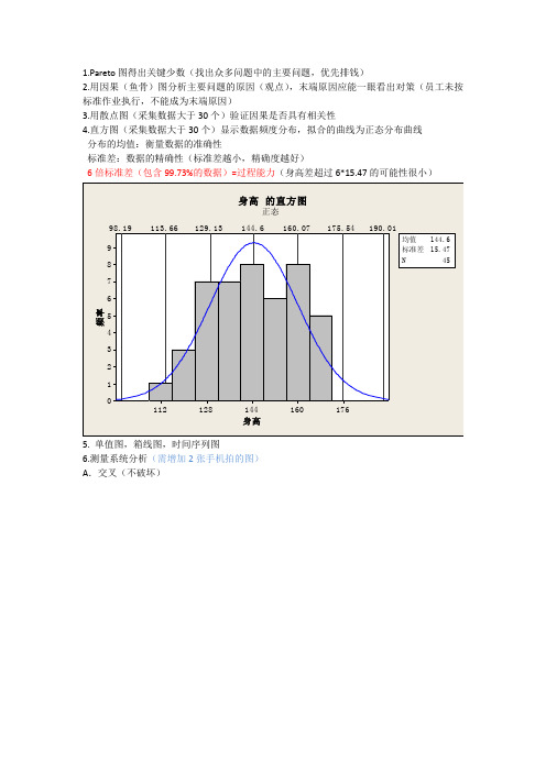
1.Pareto图得出关键少数(找出众多问题中的主要问题,优先排钱)2.用因果(鱼骨)图分析主要问题的原因(观点),末端原因应能一眼看出对策(员工未按标准作业执行,不能成为末端原因)3.用散点图(采集数据大于30个)验证因果是否具有相关性4.直方图(采集数据大于30个)显示数据频度分布,拟合的曲线为正态分布曲线分布的均值:衡量数据的准确性标准差:数据的精确性(标准差越小,精确度越好)6倍标准差(包含99.73%的数据)=过程能力(身高差超过6*15.47的可能性很小)5. 单值图,箱线图,时间序列图6.测量系统分析(需增加2张手机拍的图)A.交叉(不破坏)此图只具有参考意义测量值*测量员体现重复性来源标准差(SD) (6 * SD) 异 (%SV) (SV/Toler)合计量具 R&R 0.067596 0.40558 33.56 40.56(两者都小于10%,合格;10%~30%测量关键特性,任意一个大于30%,不合格)重复性 0.032592 0.19555 16.18 19.56再现性 0.059220 0.35532 29.40 35.53(再现性影响更大)测量员 0.028470 0.17082 14.13 17.08测量员*洗衣粉袋 0.051928 0.31157 25.78 31.16部件间 0.189745 1.13847 94.20 113.85合计变异 0.201426 1.20856 100.00 120.86产品过程可区分的类别数 = 3(可区分类别数>10,优秀;大于等于5,不合格;小于5,不及格)(衡量分辨力)综上红色字体,以上测量系统不合格B.嵌套(破坏性)嵌套式与交叉式相比,缺少再现性图过程公差 = 16研究变异 %研究变 %公差来源标准差(SD) (6 * SD) 异 (%SV) (SV/Toler)合计量具 R&R 1.59164 9.5499 42.86 59.69重复性 1.59164 9.5499 42.86 59.69 再现性 0.00000 0.0000 0.00 0.00 部件间 3.35534 20.1321 90.35 125.83 合计变异 3.71371 22.2823 100.00 139.26可区分的类别数 = 2分析同上,测量系统不合格7.测量线性研究偏倚——点线性——计数型测量系统分析评定值的属性一致性分析检验员自身(重复性)评估一致性# 检 # 相检验员验数符数百分比 95 % 置信区间钱 6 3 50.00 (11.81, 88.19)孙 6 4 66.67 (22.28, 95.67)赵 6 6 100.00 (60.70, 100.00)# 相符数: 检验员在多个试验之间,他/她自身标准一致。

Python中准确率曲线函数一、概述在机器学习中,评估模型的准确率是非常重要的一环。
准确率曲线函数能够帮助我们分析模型的性能,找出最佳的阈值,并且是一种非常直观的评估方式。
本文将介绍Python中的准确率曲线函数,包括其原理、用法和实际应用。
二、准确率曲线函数的原理准确率曲线函数是一种衡量二分类模型性能的工具,它通过绘制不同阈值下的真阳性率(True Positive Rate, TPR)和假阳性率(False Positive Rate, FPR)的变化曲线来展现模型的表现。
TPR和FPR的定义如下:TPR = TP / (TP + FN)FPR = FP / (FP + TN)其中,TP代表真阳性,FN代表假阴性,FP代表假阳性,TN代表真阴性。
通过计算不同阈值下的TPR和FPR,我们可以绘制出准确率曲线,从而分析模型的性能。
三、准确率曲线函数的用法在Python中,我们可以利用scikit-learn库中的roc_curve函数来计算准确率曲线。
该函数的使用方法如下:```pythonfrom sklearn.metrics import roc_curvefpr, tpr, thresholds = roc_curve(y_true, y_score)```其中,y_true代表真实标签,y_score代表模型的得分。
该函数将返回不同阈值下的FPR、TPR和阈值,我们可以利用这些数据来绘制准确率曲线。
四、准确率曲线函数的实际应用下面以一个实际案例来展示准确率曲线函数的应用。
假设我们有一个二分类模型,我们可以先使用该模型对测试集进行预测,然后利用roc_curve函数计算准确率曲线。
我们可以利用matplotlib库来绘制该曲线,并找出最佳阈值。
```pythonimport matplotlib.pyplot as pltplt.plot(fpr, tpr, label='ROC curve (area = 0.2f)' roc_auc)plt.plot([0, 1], [0, 1], 'k--')plt.xlim([0.0, 1.0])plt.ylim([0.0, 1.05])plt.xlabel('False Positive Rate')plt.ylabel('True Positive Rate')plt.title('Receiver Operating Characteristic')plt.legend(loc="lower right")plt.show()```通过观察准确率曲线,我们可以找出最佳阈值,从而提高模型的性能。


python的科赫曲线代码绘制三阶六边形科赫曲线是一种分形。
其形态似雪花,又称科赫雪花、雪花曲线。
它最早《关于一条连续而无切线,可由初等几何构作的曲线》科赫曲线是deRham曲线的特例。
1.给定线段AB,科赫曲线可以由以下步骤生成:
2.将线段分成三等份(AC,CD,DB)
3.以CD为底,向外(内外随意)画一个等边三角形DMC
4.将线段CD移去
分别对AC,CM,MD,DB重复1~3。
科赫雪花是以等边三角形三边生成的科赫曲线组成的。
科赫雪
花的面积是
,其中S是原来三角形的边长。
每条科赫曲线的长度是无限大,它是连续而无处可微的曲线。
画法:
1、任意画一个正三角形,并把每一边三等分;
2、取三等分后的一边中间一段为边向外作正三角形,并把这“中间一段”擦掉;
3、重复上述两步,画出更小的三角形。
4、一直重复,直到无穷,所画出的曲线叫做科赫曲线。
和皮亚诺类似:
1、曲线任何处不可导,即任何地点都是不平滑的
2、总长度趋向无穷大
3、曲线上任意两点沿边界路程无穷大
4、面积是有限的
5、产生一个匪夷所思的悖论:"无穷大"的边界,包围着有限的面积。

ROC曲线,也称为受试者工作特征曲线,主要用于评估二分类模型的性能。
绘制ROC曲线的原理主要是通过改变分类模型的判定阈值,计算各个阈值下的真正例率(TPR)和假正例率(FPR),并将这些点连接起来形成曲线。
在Python中,可以使用scikit-learn库中的roc_curve和auc函数来绘制和计算ROC曲线。
具体步骤如下:1. 准备数据:包括测试集的标签(真实值)和模型预测的概率得分。
2. 利用roc_curve函数计算FPR和TPR:该函数需要两个参数,分别是模型预测的概率得分和测试集标签。
返回的结果还包括阈值。
3. 计算AUC:使用auc函数,将FPR和TPR作为输入参数,得到ROC曲线下的面积(AUC)。
以下是一段示例代码:```pythonfrom sklearn.metrics import roc_curve, aucimport matplotlib.pyplot as plt# 假设y_test为测试集结果,scores为模型预测的得分y_test = [0, 0, 1, 1]scores = [0.1, 0.4, 0.35, 0.8]# 计算roc_curvefpr, tpr, thresholds = roc_curve(y_test, scores)# 计算aucroc_auc = auc(fpr, tpr)# 绘制roc曲线plt.figure()lw = 2plt.plot(fpr, tpr, color='darkorange', lw=lw, label='ROC curve (area = %0.2f)' % roc_auc)plt.plot([0, 1], [0, 1], color='navy', lw=lw, linestyle='--')plt.xlim([0.0, 1.0])plt.ylim([0.0, 1.05])plt.xlabel('False Positive Rate')plt.ylabel('True Positive Rate')plt.title('Receiver operating characteristic example')plt.legend(loc="lower right")plt.show()```这段代码将绘制出一个ROC曲线,并计算出AUC值。

我的一次实验记忆巧克力英语作文Chocolate, a delectable confectionery delight, has captivated the palates of countless individuals across the globe for centuries. Its rich, complex flavor and velvety texture evoke a symphony of sensations, leaving an unforgettable impression on the human gustatory experience.As a curious and eager student, I embarked on an experiment to delve into the intricate world of chocolate, unraveling its secrets and exploring its captivating allure. My objective was to conduct a memory experiment toascertain the extent to which the consumption of chocolate influenced my ability to recall information.I designed a rigorous experimental protocol, meticulously controlling all variables that couldpotentially confound the results. The experiment consistedof two phases: a study phase and a test phase. During the study phase, I presented participants with a series of unfamiliar words and paired them with either chocolate or aneutral control substance. The chocolate condition involved consuming a small piece of dark chocolate, approximately 10 grams, while the control condition involved consuming a piece of unsweetened cracker.After a brief interval, participants entered the test phase, where they were asked to recall as many words as possible from the study phase. The number of wordscorrectly recalled was recorded for each participant in both the chocolate and control conditions.The results of my experiment yielded intriguinginsights into the relationship between chocolate consumption and memory. Statistical analysis revealed that participants who consumed chocolate during the study phase exhibited a significant improvement in their ability to recall words compared to those who consumed the neutral control substance. This finding suggests that chocolate may possess memory-enhancing properties, potentially due to its high concentration of flavonoids, which have been associated with improved cognitive function.To further validate my findings, I conducted a comprehensive literature review, delving into the existing body of research on the effects of chocolate on memory. Numerous studies have reported similar positive outcomes, indicating that chocolate consumption can enhance both short-term and long-term memory performance.One particularly compelling study, published in the journal "Appetite," investigated the impact of chocolate on episodic memory, which refers to the ability to recall specific events and experiences. The researchers found that participants who consumed chocolate prior to a memory task performed significantly better than those who consumed a placebo. This study suggests that chocolate may improve the encoding and consolidation of memories, leading to enhanced recall later on.Another study, published in the journal "Neurology," examined the relationship between chocolate consumption and cognitive decline in older adults. The researchers followed a group of elderly participants for several years, tracking their chocolate consumption and cognitive function. Theyfound that participants who consumed chocolate regularly had a lower risk of developing cognitive impairment and dementia compared to those who did not consume chocolate. This finding suggests that chocolate may have neuroprotective properties that help to preserve cognitive function as we age.In addition to its potential memory-enhancing effects, chocolate has also been linked to a number of other health benefits. For instance, chocolate contains high levels of antioxidants, which can help to protect cells from damage caused by free radicals. Some studies have also suggested that chocolate may improve cardiovascular health by lowering blood pressure and reducing the risk of blood clots.Overall, the evidence suggests that chocolate, particularly dark chocolate with a high cocoa content, offers a unique combination of culinary delight and potential health benefits. While further research is needed to fully understand the mechanisms by which chocolate exerts its effects on memory and other cognitive functions,the current findings provide a tantalizing glimpse into the potential of this delectable treat to enhance our cognitive abilities.In conclusion, my experiment, coupled with the wider body of research, provides compelling evidence that chocolate consumption can enhance memory performance. Whether enjoyed as a sweet indulgence or incorporated into a healthy diet, chocolate appears to possess cognitive-boosting properties that make it a delectable and potentially beneficial addition to our daily lives.。
validation_curve()的用法在机器学习的模型调参过程中,我们经常会用到模型的验证曲线。
而scikit-learn库中的validation_curve()功能就是用于产生模型验证曲线的。
本文将围绕validation_curve()的用法进行详细的阐述。
1. validation_curve()函数的定义validation_curve()函数可以用于生成模型的验证曲线。
该函数最常用的参数是estimator,param_name和param_range,其含义如下:- estimator: 机器学习算法,能够直接应用于数据集并进行学习的对象。
- param_name: 算法可调整参数的名称。
- param_range:算法可调整参数的取值范围。
同时,validation_curve()函数也可以接受一系列其他的输入参数,如train_scores,test_scores和error_score等,这些参数的默认值由sklearn.model_selection.validation_curve提供。
2. validation_curve()函数的用法接下来我们通过一个例子来详细阐述validation_curve()函数的用法。
下面是一份用于分类任务的Iris数据集:```from sklearn.datasets import load_irisfrom sklearn.model_selection import validation_curvefrom sklearn.neighbors import KNeighborsClassifierimport matplotlib.pyplot as pltiris = load_iris()X, y = iris.data, iris.targetparam_range = range(1, 20, 2)train_scores, test_scores = validation_curve(KNeighborsClassifier(),X, y,param_name='n_neighbors',param_range=param_range,cv=10)train_mean = np.mean(train_scores, axis=1)test_mean = np.mean(test_scores, axis=1)plt.plot(param_range, train_mean, label='Training score', color='blue')plt.plot(param_range, test_mean, label='Cross Validationscore', color='red')plt.legend(loc='best')plt.xlabel('n_neighbors')plt.ylabel('Score')plt.show()```在上述代码中,我们首先引入了必需的模块,然后定义Iris数据集并加载数据。
题目:探究Python误差曲线与置信区间的相关性一、概述Python作为一种广泛应用的编程语言,在数据分析和统计学领域也有着重要的地位。
误差曲线和置信区间是统计学中常见的概念,对于数据分析和结果解释具有重要意义。
本文将探讨Python中误差曲线与置信区间的相关性,希望能够为相关领域的研究者和实践者提供参考。
二、Python中的误差曲线1. 误差曲线的定义误差曲线是指在统计数据中,用来表示平均值附近的变化范围的一条曲线。
在Python中,我们可以使用matplotlib库来绘制误差曲线,通过展示数据的波动范围,能够更直观地理解数据的分布特征。
2. Python绘制误差曲线的方法在Python中,我们可以使用matplotlib库的errorbar函数来绘制误差曲线,该函数能够展示数据点与其对应的误差范围,使得数据的波动情况一目了然。
3. 误差曲线的应用误差曲线在数据分析和统计学中具有重要的应用,能够帮助研究者对数据进行更全面的分析和解释。
在科研领域和实际应用中,误差曲线能够有效地辅助决策和结果评估。
三、Python中的置信区间1. 置信区间的定义置信区间是指用来估计总体参数的区间估计方法,它表示了参数估计的不确定性范围。
在Python中,我们可以使用scipy库来计算数据的置信区间,从而对数据的总体特征进行推断。
2. Python计算置信区间的方法使用scipy库中的stats模块,可以方便地计算数据的置信区间。
通过指定置信水平和样本数据,即可得到数据的置信区间范围,从而更准确地评估统计结论的可靠性。
3. 置信区间的应用置信区间是统计学中常用的工具,能够帮助研究者对样本数据进行推断,并对总体特征进行估计。
在实际应用中,置信区间的计算结果能够有效地指导决策和结论的推断。
四、Python中的误差曲线与置信区间的关联1. 误差曲线与置信区间的概念通联误差曲线和置信区间在统计学中都与数据的不确定性和可靠性有关。
python nrubs 曲线拟合-概述说明以及解释1.引言1.1 概述概述本文将介绍Python中NRubs曲线拟合的概念和应用。
在现实生活和工作中,我们经常需要通过一系列数据点来近似表示一个曲线。
NRubs 曲线拟合是一种数学方法,可用于找到一个平滑的曲线,以最佳地逼近给定的数据点。
Python作为一种高级编程语言,提供了许多强大的工具和资源,使我们能够轻松地进行数据处理和曲线拟合。
本文将首先介绍Python的基础知识,包括数据结构、变量和函数等方面的内容。
然后,我们将深入探讨NRubs曲线拟合的概念。
NRubs曲线拟合是一种基于样条函数的方法,通过将给定的数据点与多项式函数相连,生成一条平滑的曲线。
在理解NRubs曲线拟合的原理和数学模型之后,我们将学习如何在Python中应用这种方法。
在正文部分,我们将详细介绍Python中的NRubs曲线拟合的实现步骤和技巧。
通过使用Python的相关库和函数,我们可以轻松地进行数据处理、拟合曲线并可视化结果。
在结论部分,我们将总结本文的主要内容,并探讨NRubs曲线拟合在实际应用中的潜力和局限性。
我们将指出NRubs曲线拟合的优点和不足之处,并提出如何进一步改进和应用这种方法的建议。
通过本文的学习,读者将掌握Python中NRubs曲线拟合的基本原理和实践技巧。
有了这些知识,读者可以更好地应用NRubs曲线拟合解决实际问题,并在数据分析和科学研究领域中发挥更大的作用。
1.2 文章结构文章结构部分的内容可以包括以下内容:文章结构部分旨在介绍整篇文章的组织架构和内容安排,以便读者能够更好地理解文章的组成和流程。
下面将详细介绍本文的结构。
本文分为引言、正文和结论三个部分。
1. 引言部分(Introduction):主要对本文的主题进行概述,简要介绍Python和NRubs曲线拟合的基本概念和应用。
首先,通过引入Python 的基础知识,为读者提供了解Python编程语言的必要背景。
a r X i v :0710.1097v 1 [a s t r o -p h ] 4 O c t 2007Curious Variables Experiment (CURVE).CCD Photometry of V419Lyr in its 2006July Superoutburst.A.R u t k o w s k i 1, A.O l e c h 1,K.M u l a r c z y k 2, D.B o y d 3,R.K o f f 4and M.W i ´s n i e w s k i 11Nicolaus Copernicus Astronomical Center,Polish Academy of Sciences,ul.Bartycka 18,00-716Warszawa,Poland,e-mail:(rudy,olech,mwisniew)@.pl 2Warsaw University Observatory,Al.Ujazdowskie 4,00-476Warszawa,Poland,e-mail:kmularcz@.pl 3British Astronomical Association,Variable Star Section,West Challow OX129TX,England e-mail:drsboyd@ 4Antelope Hills Observatory,980Antelope Drive West,Bennett,CO 80102,USA e-mail:bob@ Abstract We report extensive photometry of the dwarf nova V419Lyr throughout its 2006July superoutburst till quiescence.The superoutburst with amplitude of ∼3.5magnitude lasted at least 15days and was characterized by the presence of clear superhumps with a mean period of P sh =0.089985(58)days (129.58±0.08min).According to the Stolz-Schoembs relation,this indicates that the orbital period of the binary should be around 0.086days i.e.within the period gap.During the superoutburst the superhump period was decreasing with the rate of ˙P/P sh =−24.8(2.2)×10−5,which is one of the highest values ever observed in SU UMa systems.At the end of the plateau phase,the superhump period stabilized at a value of 0.08983(8)days.The superhump amplitude decreased from 0.3mag at the beginning of the superoutburst to 0.1mag at its end.In the case of V419Lyr we have not observed clear secondary humps,which seems to be typical for long period systems.Key words:Stars:individual:V419Lyr –binaries:close –novae,cataclysmic variables1IntroductionDwarf novae –a subclass of Cataclysmic Variable stars –are quite well studied interacting binary systems composed of late-type red dwarf secondary and white dwarf primary stars (Warner 1995,Hellier 2001).Matter transferred from the red dwarf forms an accretion disc around the white dwarf.Although in the last decade significant progress has been made in explaining the behaviour of dwarf novae light curves,some physical pro-cesses ongoing in these systems are still not fully understood (see for example Smak 2000,Schreiber and Lasota 2007).In particular,the thermal-tidal instability model of Osaki (1996,2005)describing the phenomenon ofsuperoutbursts and superhumps may be tested by examination of SU UMa-type dwarf novae light curves.Ad-ditionally,objects near and inside the so called period gap are very important from an evolutionary point of view.Those systems give us an unprecedented opportunity to study the evolution of dwarf novae.V419Lyr is a poorly studied cataclysmic variable discovered by Kurochkin(1990)and originally classified as a Z Cam-type dwarf ter,Nogami et al.(1998)caught this object in outburst and found superhumps in its light curve.Detection of superhumps together with characteristic properties of the outburst allowed them to classify V419Lyr as a SU UMa-type dwarf nova,but short coverage of the eruption did not allow accurate determination of the superhump period.Nevertheless,there was a strong suggestion that V419Lyr has one of the longest orbital periods known among SU UMa variables.This object has been monitored at various photometric bands by the Variable Star Network(VSNET)(see for example Kato et al.2004a).The observations from that program enabled a tentative determination of the supercycle period to be about∼340days(Katysheva and Pavlenko2003).Moreover,Morales-Rueda and Marsh(2002)obtained a spectrum of V419Lyr during outburst showing a relatively broad absorption feature around430-440nm.In this work we present an analysis of photometric data collected during the2006July superoutburst of V419Lyr.The data are much richer than previous studies and provide us with an opportunity to determine parameters describing this system more precisely.2Observations and data reductionThe CURious Variable Experiment(CURVE)team(see for example Olech et al.2004,2006),alerted by the VSNET mailing list,found V419Lyr in a very bright state on2006July17/18.Subsequently the object was monitored on13consecutive nights(with a gap on July24/25)until its return to quiescence on August2/3. The observations were performed using a0.6-m Cassegrain telescope equipped with a Tektronix TK512CB back-illuminated CCD camera.The image scale was0′′.76/pixel providing a6′.5×6′.5field of view(Udalski and Pych,1992)Observations were made unfiltered for two reasons.First,due to lack of an autoguiding system,we wished to keep exposures short in order to minimize guiding errors.Second,because our main goal was analysis of the temporal behaviour of the light curve,the use offilters might cause the object to be too faint to observe in quiescence.Exposure times were90seconds during the bright state and100-150seconds at minimum light.All CURVE team data reductions were performed using a standard procedure based on IRAF1package and the profile photometry has been derived using the DAOphotII package(Stetson1987).During preliminary analysis of the data we found the AA VSO archive containing several CCD observations of the same superoutburst of V419Lyr made by observers from England(D.B.)and the United States(R.K.). Therefore we decided to combine our data to obtain better results.ed a0.35-m Meade Schmidt-Cassegrain telescope with a Starlight Xpress SXV-H9CCD camera. Data were taken unfiltered.Exposures were40,50or60sec depending on conditions.The AIP4WIN package (Berry and Burnell2000)was used to dark-subtract andflat-field all images before measuring them using aperture photometry.The magnitude of V419Lyr was determined by differential photometry with respect to an ensemble of two nearby comparison stars.ed0.25-m Meade LX-200Schmidt-Cassegrain telescope equipped with an Apogee AP-47CCD camera and clearfilter characterized by IR block at700nm.MPO Canopus software(Warner2007)was used for differential photometry of the variable with an average of four comparison stars.Table1presents a journal of our CCD observations of V419Lyr.In total,we observed the star for more than48hours on14nights and collected3179exposures.Table1:Observational journal for the V419Lyr campaign.O.Start and O.End correspond(for particular nights)to times forfirst and last CCD frame made in Ostrowik observatory.D.B./R.K.Start and D.B./R.K End correspond to data obtained by David Boyd and Robert Koff respectively."Dur."Gives the total duration of runs from all telescopes excluding the gaps.Date in O.Start O.End D.B.Start D.B.End R.K.Start R.K.End Dur.No.of<V> 20062453000+2453000+2453000+2453000+2453000+2453000+[hr]points[mag]3Global light curveFigure1presents the photometric behaviour of V419Lyr in2006July and August.Dots and open circles correspond to our CCD observations and visual estimates of AA VSO observers,respectively.14.515.51616.5V1717.51818.5935 940 945 950HJD-2453000Figure1:Global light curve of2006superoutburst of V419Lyr.Dots and open circles denote our observa-tions and AAVSO estimates,respectively.Solid line is a least squares linearfit to the plateau phase of the superoutburst.The shape of the light curve corresponds to the standard picture of a superoutburst.First,the star rose rapidly from its quiescent level to a peak magnitude of around14.5mag.Due to the lack of observations,theexact time of the rise is unknown.V419Lyr was seen by AA VSO observers in a bright state on July 16.Two nights later,during our first run,the star was still at the same brightness and showing fully developed super-humps with a peak-to-peak amplitude of 0.3mag -a feature characteristic of the beginning of a superoutburst.Thus we conclude that the July 2006superoutburst started around July 15.-0.2-0.10.1-0.2-0.10.1-0.2-0.10.1-0.2-0.10.1-0.2-0.10.1-0.2-0.10.1-0.2-0.10.10.350.400.450.500.55D e t r e n d e d r e l a t i v e m a g n i t u d e Fraction of the HJD0.350.400.450.500.55-0.2-0.10.1-0.2-0.10.10.600.700.800.90Fraction of the HJD0.600.700.800.90Figure 2:Superhumps observed each night during the 2006July superoutburst of V419Lyr.After reaching peak magnitude,V419Lyr entered the plateau stage lasting about 11days with an average decline rate of about 0.1mag d −1.The plateau stage ended rapidly on July 27and during the next two days we observed the final decline stage with a change of brightness of about 1mag d −1.On July 30the star was again in quiescence showing a mean brightness of 18.1mag.Thus the entire superoutburst lasted about 15days.The linear fit to the plateau stage in Figure 1is helpful in showing there was no rebrightening as has beenobserved in some SU UMa systems (Kato et al.2003a).4SuperhumpsFigure 2shows the light curves of V419Lyr during thirteen individual nights.Filled circles correspond to the Ostrowik Observatory data,while open circles and squares represent D.B.and R.K.measurements respectively.The magnitudes have been transformed to a common V system and detrended for purposes of Fourier power spectrum analysis.The superhumps are clearly visible and have an initial amplitude of ter the superhump amplitude gradually decreases and on August 2/3is practically indistinguishable from noise.4.1ANOV A statisticsAs we noted earlier,all light curves of V419Lyr in superoutburst were detrended by removing a fit based on a first or second order polynomial.Then we analyzed them using ANOVA statistics (Schwarzenberg-Czerny 1996).The resulting periodogram is shown in Figure 3.It shows a very clear and dominant peak at fre-quency f 0=11.107±0.010c/d,which we interpret as due to superhumps and corresponds to the period P sh =0.09033(81)days.1002003004005004 8 12 1620 24A N O V A s t a t .Frequency [c/d]f 0=11.107 c/d Figure 3:ANOVA power spectrum computed for data from nights July 17/18-July 27/28.The spectrum has almost no 1-day aliases due to good coverage and the use of data from three sites -two from Europe and one from the United States.A small peak is also observed around 22c/d,the first harmonic of the main frequency.We then prewhitened the light curve of V419Lyr during the superoutburst with the main period and its first harmonic.The power spectrum of the resulting light curve shows no other periodicities.4.2The O-C analysisTo check the stability of the superhump period and to better determine its value,we constructed an O −C diagram.Because the maxima in our case were almost always clearly visible and easier to measure than minima,we decided to use the timings of the former.Finally,we were able to determine 27times of maxima which are listed in Table 2together with associated errors,cycle numbers E ,and O −C values.Table2:Times of maxima observed in the light curve of V419Lyr during its2006superoutburstCycle HJD-2453000Error O-CA least-squares linearfit to the data taken during the plateau phase of superoutburst gives the following ephemeris for the maxima:HJD max=2453934.4326(41)+0.089983(58)·E(1) The above equation indicates that the mean superhump period was P sh=0.089983(58)days,which agrees within errors with the determination based on ANOVA bining these two measurements gives us ourfinal estimate of the mean superhump period of V419Lyr during its2006July superoutburst which is P sh=0.089985(58)days(129.58±0.08min).The O−C values computed according to the ephemeris(1)are listed in Table2and also shown in Figure4. It is clear that V419Lyr,during its2006superoutburst,showed clear changes of superhump period.In the cycle range0−70the period was quickly decreasing.A second-order polynomialfit to E vs.HJD max dependence in this range corresponds to the solid line in the bottom panel of Figure4and is expressed by the following ephemeris:HJD max=2453934.42496(117)+0.0908080(75)·E−1.125(97)·10−5·E2(2) This equation indicates that the period derivative has the large value˙P/P sh=−24.8(2.2)×10−5.This isthe second largest negative value detected in SU UMa stars.Figure 5,taken from Kato et al.(2003b)and Olech et al.(2003),shows the position of V419Lyr on the ˙P/P sh vs P sh diagram.Only KK Tel had a faster period decrease during its 2002June superoutburst (Kato et al.2003b).It is interesting that both V419Lyr and KK Tel are long superhump period dwarf novae with orbital periods very close or even within the period gap.-0.2-0.10 0.1 0.2 0.3 0 20 40 60 80 100 120 140 160O -C [c y c l e s ]E0.10.20.3A m p l i t u d e [m a g ]935938941944947HJD - 2453000Figure 4:Upper panel:Evolution of the amplitude of superhumps observed in the 2006July superoutburst of V419Lyr.Lower panel:O −C diagram for times of superhump maxima.Solid line corresponds to the quadratic ephemeris (2).Black and open squares denote normal and late superhump maxima respectively.Dashed line corresponds to the 5th order polynomial fit.Size of the squares is,on average,of the size of error bars.-40-200 200.04 0.06 0.08 0.1 0.12d P /d t (×10-5)Superhump period [d]It is worth commenting on the behaviour of the superhump period after cycle number E =70.At that moment,the star was still in the plateau phase of the superoutburst,three days before entering the final decline,and superhumps were still clearly visible in the light curve.The O −C values for cycle numbers from 70toFigure5:˙P/P sh versus P sh for SU UMa-type dwarf novae.Thefigure is taken from Kato et al.(2003b)and Olech et al.(2003).P min denotes the boundary for a hydrogen rich secondary.The range of the period gap is also plotted.1RXS is an abbreviation for1RXS J232953.9+062814.111can be roughlyfitted with a straight line,which indicates that the period decrease had stopped and its value stabilized at P sh=0.08983(8)days.The noisy maxima with cycle numbers above120are shifted by∼0.4cycle with respect to the superhump maxima from earlier nights.This indicates that they may be connected with late superhumps or even with the orbital wave.It is interesting that our O−C diagram could be also interpreted in diffrent way than"common superhump followed by transition to late superhump"scenario.Fitting a5th order polynomial to the moments of maxima appears to work with the data about as well as a quadratic followed by a linear trend as described previously. We are not arguing in favour of this interpretation,simply saying that there might be other interpretations of the data.4.3Amplitude and shapeThe upper panel of Figure4shows the evolution of the amplitude of superhumps through the entire super-outburst.In a typical SU UMa star,fully developed superhumps have an amplitude of about0.3mag and a characteristic tooth shape.Interestingly,these properties seem to be completely independent of the inclination of the orbit of the binary.As the outburst progresses,the amplitude gradually decreases and the profile of the humps changes.A few days after maximum,so called secondary humps or interpulses become visible.In the beginning they are small but with time they may become as high as the main maxima-most probably evolving towards late superhumps.V419Lyr is an interesting case because it seems not to follow this scenario.On the nights of July19/20 and20/21it clearly showed double maxima.However,these quickly disappeared.During subsequent nights there was hardly a trace of secondary humps.Very weak humps could be seen only on July23/24and25/26 and quite strong ones on July27/28.We were curious about the reason for such behaviour.The only property which strongly differs in V419Lyr from typical SU UMa stars is its long superhump/orbital period placing it within the period gap.We therefore reviewed the literature to investigate the occurrence of secondary humps among long period systems(i.e.with superhump period>0.08days).The summary of our review is given in Table3.Among21reviewed stars only four show clear secondary humps.The rest of them show no interpulses at all or only a weak trace of them.5ConclusionsThe orbital period of V419Lyr is unknown.However it is possible to estimate its value using the relation in Stolz and Schoembs(1984)connecting the period excessεdefined as P sh/P orb−1with the orbital period of the binary.This empirical relation is as follows:ε=0.858(11)·P orb−0.0282(2)(3) Using the definition ofεand knowing P sh for V419Lyr,we were able to estimate the orbital period as P orb≈0.086days.This is slightly longer than two hours which indicates that V419Lyr is a dwarf nova in the period gap.Table3:Occurrence of secondary humps in long period superhumpersStar P sh[days]Clear Poorly Invisible Ref1.Kato et al.(1998),2.Kato et al.(2001),3.Woudt&Warner(2001),4.Kato et al.(2002),5.Olech et al.(2005),6.Harvey et al.(1995),7.Mennickent&Sterken(1998),8.O’Donoghue(1987),9.Kato et al.(2003c),10.Kato et al.(2004b),11.Kato&Uemura(2001),12.Nogami et al.(1995),13.Kato(2002),14.Howell et al.(1993),15.Barwig et al.(1982),16.Warner et al.(1989),17.Kato et al.(2003c),18.Kato et al.(2003b),19.Nogami et al.(2001),20.Feline et al.(2004),21.Nogami et al.(1998),22.Kato&Uemura(2001),23.Kato(1993),24.Patterson(1979),25.Kato(2001),26.Nogami et al.(1998),27.Uemura et al.(2001),28.Antipin&Pavlenko(2002),29.Nogami et al.(2003)Many characteristics of V419Lyr are typical of SU UMa stars.It goes into superoutburst every year or so,the eruption lasts about two weeks and has an amplitude of∼3.5mag.Superhumps appear shortly after the beginning of the superoutburst and have a maximum amplitude of0.3mag,which decreases to0.1mag at the end of the outburst.In addition to its long orbital period,V419Lyr is unusual in two other properties.Its superhump period derivative has one of the largest negative values known and it shows only a weak trace of secondary humps in thefinal stages of the superoutburst.Acknowledgments.We acknowledge generous allocation of the Warsaw Observatory0.6-m telescope time. This work used the online service of the VSNET and AA VSO.We would like to thank Prof.Józef Smak for fruitful discussions.References[1]Antipin,S.V.,&Pavlenko,E.P.2002,Astron.Astrophys.,391,565[2]Barwig,H.,Kudritzki,R.P.,V ogt,N.,&Hunger,K.1982,Astron.Astrophys.,114,L11[3]Berry R.,Burnell J.2000,The Handbook of Astronomical Image Processing,Willmann-Bell[4]Feline,W.J.,Dhillon,V.S.,Marsh,T.R.,&Brinkworth,C.S.2004,MNRAS,355,1[5]Harvey,D.,Skillman,D.R.,Patterson,J.,&Ringwald,F.A.1995,PASP,107,551[6]Hellier,C.2001,Cataclysmic Variable Stars,Springer[7]Howell,S.B.,Schmidt,R.,Deyoung,J.A.,Fried,R.,Schmeer,P.,&Gritz,L.1993,PASP,105,579[8]Kato,T.1993,PASJ,45,L67[9]Kato,T.,Nogami,D.,Masuda,S.,&Baba,H.1998,PASP,110,1400[10]Kato,T.,Sekine,Y.,&Hirata,R.2001,PASJ,53,1191[11]Kato,T.,&Uemura,M.2001,Informational Bulletin on Variable Stars,5158,1[12]Kato,T.2001,Informational Bulletin on Variable Stars,5104,1[13]Kato,T.,et al.2002,Astron.Astrophys.,395,541[14]Kato,T.2002,PASJ,54,87[15]Kato,T.,Nogami,D.,Moilanen,M.,Yamaoka,H.2003a,PASJ,55,989[16]Kato,T.,et al.2003b,MNRAS,339,861[17]Kato,T.,Bolt,G.,Nelson,P.,Monard,B.,Stubbings,R.,Pearce,A.,Yamaoka,H.,Richards,T.2003c,MNRAS,341,901[18]Kato,T.,Uemura,M.,Ishioka,R.,Nogami,D.,Kunjaya,C,Baba,H.,Yamaoka,H.2004a,PASJ,56,1[19]Kato,T.,et al.2004b,MNRAS,347,861[20]Katysheva,N.A.,Pavlenko,E.P.2003,Astophysics,46,114[21]Kuroshkin,N.E.1990,Peremennye Zvezdy,17,186[22]Mennickent,R.E.,&Sterken,C.1998,PASP,110,1032[23]Nogami,D.,Kato,T.,Masuda,S.,&Hirata,R.1995,Informational Bulletin on Variable Stars,4163,1[24]Nogami,D.,Kato,T.,&Masuda,S.1998,PASJ,50,411[25]Nogami,D.,Kato,T.,Baba,H.,Novák,R.,Lockley,J.J.,Somers,M.2001,MNRAS,322,79[26]Nogami,D.,et al.2003,Astron.Astrophys.,404,1067[27]O’Donoghue,D.1987,Astrophys.Space Science,136,247[28]Olech,A.,Schwarzenberg-Czerny,A.,Kedzierski,P.,Zloczewski,K.,Mularczyk,K.,Wisniewski,M.2003,Acta Astron.,53,175[29]Olech,A.,Zloczewski,K.,Mularczyk,K.,Kedzierski,P.,Wisniewski,M.,Stachowski,G.2004,ActaAsron.,54,57[30]Olech,A.,Zloczewski,K.,Cook,L.M.,Mularczyk,K.,Kedzierski,P.,Wisniewski,M.2005,ActaAstron.,55,237[31]Olech,A.,Mularczyk,K.,Kedzierski,P.,Zloczewski,K.,Wisniewski,M.,Szaruga,K.2006,Astron.Astrophys.,452,933[32]Osaki,Y.1996,PASP,108,39[33]Osaki,Y.2005,Proc.of the Japan Academy,Seires B,81,291[34]Patterson,J.1979,Astron.J.,84,804[35]Schreiber,M.R,Lasota,J.-P.2007,arXiv:0706.3888[36]Schwarzenberg-Czerny,A.1996,ApJ Letters,460,L107[37]Smak,J.2000,New Astronomy,44,171[38]Stetson,P.B.1987,PASP,99,191[39]Stolz,B.,Schoembs,R.1984,Astron.Astrophys.,132,187[40]Udalski A.,Pych W.1992,Acta Astron.,42,285[41]Uemura,M.,Kato,T.,Pavlenko,E.,Baklanov,A.,&Pietz,J.2001,PASJ,53,539[42]Warner,B.,O’Donoghue,D.,&Wargau,W.1989,MNRAS,238,73[43]Warner B.1995,Cataclysmic Variable Stars,Cambridge University Press.[44]Warner B.2007,/MPOSoftware/MPOCanopus.htm[45]Woudt,P.A.,&Warner,B.2001,MNRAS,328,15911。