第十章小角激光散射
- 格式:ppt
- 大小:2.80 MB
- 文档页数:55


一、实验目的1. 理解小角激光散射的基本原理和实验方法;2. 通过实验观察和测量,了解聚合物球晶的形态和尺寸;3. 掌握数据处理和分析方法,对实验结果进行解释。
二、实验原理小角激光散射(Small Angle Laser Scattering,简称SALS)是一种研究材料微观结构的方法。
当一束激光照射到材料表面时,部分光会被散射。
散射光的角度与材料内部结构的尺寸和形态有关。
通过测量散射光的强度和角度,可以推断出材料内部结构的特征。
小角激光散射实验的基本原理如下:1. 当激光束照射到样品上时,部分光会被样品散射;2. 散射光经过透镜聚焦后,形成散射光斑;3. 通过测量散射光斑的直径和强度,可以计算样品内部结构的尺寸和形态。
三、实验仪器与材料1. 实验仪器:小角激光散射仪、样品台、计算机、数据采集卡等;2. 实验材料:聚合物球晶样品。
四、实验步骤1. 样品制备:将聚合物球晶样品切成薄片,厚度约为1mm;2. 样品安装:将样品放置在样品台上,调整样品位置,确保样品中心位于激光束照射范围内;3. 数据采集:打开小角激光散射仪,调整激光束照射角度和功率,采集散射光斑的直径和强度;4. 数据处理:将采集到的数据输入计算机,进行数据处理和分析;5. 结果分析:根据数据处理结果,分析聚合物球晶的形态和尺寸。
五、实验结果与分析1. 散射光斑直径:通过测量散射光斑的直径,可以计算出聚合物球晶的尺寸。
实验结果显示,聚合物球晶的尺寸约为50μm;2. 散射光斑强度:散射光斑的强度与聚合物球晶的形态有关。
通过分析散射光斑强度,可以推断出聚合物球晶的形态。
实验结果显示,聚合物球晶的形态为球形;3. 数据处理与分析:将实验数据输入计算机,进行数据处理和分析。
通过分析散射光斑的直径和强度,可以得出聚合物球晶的尺寸和形态。
六、实验结论1. 通过小角激光散射实验,成功观察和测量了聚合物球晶的形态和尺寸;2. 实验结果表明,聚合物球晶的尺寸约为50μm,形态为球形;3. 小角激光散射实验是一种有效的研究材料微观结构的方法,可以应用于聚合物、生物大分子、非晶合金等多种材料。
一、什么是X射线小角散射一种区别于X射线大角(2θ从5 ~165 )衍射的结构分析方法。
利用X射线照射样品,相应的散射角2θ小(5 ~7 ),即为X射线小角散射。
二、X射线小角散射的用途用于分析特大晶胞物质的结构分析以及测定粒度在几十个纳米以下超细粉末粒子(或固体物质中的超细空穴)的大小、形状及分布。
对于高分子材料,可测量高分子粒子或空隙大小和形状、共混的高聚物相结构分析、长周期、支链度、分子链长度的分析及玻璃化转变温度的测量。
三、X射线小角散射的原理小角散射效益来自物质内部1~l00nm量级范围内电子密度的起伏,当一束极细的x射线穿过一超细粉末层时,经粉末颗粒内电子的散射,X射线在原光束附近的极小角域内分散开来,其散射强度分布与粉末粒度及分布密切相关。
20世纪初,伦琴发现了比可见光波长小的辐射。
由于对该射线性质一无所知,伦琴将其命名为X射线(X-ray)。
到20世纪30年代,人们以固态纤维和胶态粉末为研究物质发现了小角度X射线散射现象。
当X射线照射到试样上时,如果试样内部存在纳米尺度的电子密度不均匀区,则会在入射光束周围的小角度范围内(一般2=<6º)出现散射X射线,这种现象称为X射线小角散射或小角X 射线散射(Small Angle X-ray Scattering),简写为SAXS 。
其物理实质在于散射体和周围介质的电子云密度的差异。
SAXS已成为研究亚微米级固态或液态结构的有力工具。
横坐标是散射峰的位置,纵坐标是散射峰的强度,这一点与XRD是类似的。
纵坐标的绝对数值没有意义,只是表示相对的强度。
而对于横坐标,XRD的位置通常用角度ө或2ө标示,而SAXS的位置是用q 标示的,q一般叫做散射矢量或者散射因子,q与ө有简单的换算关系q = 4πsinө/λ。
在SAXS中由于ө的数值变化范围很小,所以用q标示更方便。
在XRD中,衍射峰对应的ө可以换算出对应的晶面间距,实际上就是样品中一定范围内的周期性长度。


实验七 小角激光光散射法测定 全同立构聚丙烯球晶半径小角激光光散射(Small Angle Laser Scattering ,以下简称SALS )法被广泛地用来研究聚合物薄膜、纤维中的结构形态及其拉伸取向、热处理过程结构形态的变化、液晶的相态转变等,已成为研究聚合物结构与性能关系的重要方法。
SALS 表征的聚合物结构单元的大小在10-10m 到10-8m 之间。
一、实验目的:用小角激光光散射法研究聚合物的球晶,并了解有关原理。
二、基本原理:根据光散射理论,当光波进入物体时,在光波电场作用下,物体产生极化现象, 出现由外电场诱导而形成的偶极矩。
光波电场是一个随时间变化的量,因而诱导偶极矩也就随时间变化而形成一个电磁波的辐射源,由此产生散射光。
光波在物体中的散射,根据谱频的3个频段,可分为瑞利(Rayleigh )散射,拉曼(Raman )散射和布里渊(Brillouin )散射等。
而SALS 方法是可见光的瑞利散射。
它是由于物体内极化率或折射率的不均一性引起的弹性散射,即散射光的频率与入射光的频率完全相同(拉曼散射和布里渊散射都涉及到频率的改变)。
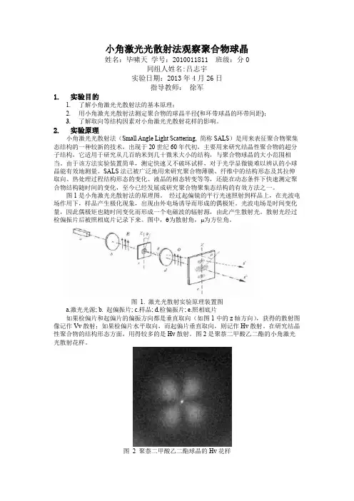
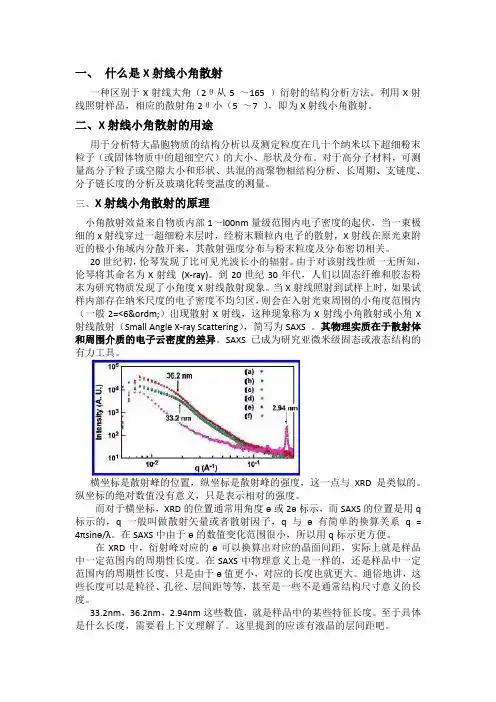
图7-1为SALS 法原理示意图。
当在起偏镜和检偏镜之间放入一个结晶聚合物样品时,入射偏振光将被样品散射成某种花样图。
图中的θ角为入射光方向与被样品散射的散射光方向之间的夹角,简称为散射角,μ角为散射光方向在YOZ 平面(底片平面)上的投影与Z 轴方向的夹角,简称方位角。
当起偏镜与检偏镜的偏振方向均为垂直方向时,得到的光散射图样叫做V V 散射,当两偏光镜正交时,得到的光散射图叫做V H 散射。
图7-1所示即V H 散射。
对SALS 散射图形的理论解释目前有模型法和统计法两种。
所谓模型法,是斯坦和罗兹(Rhodes )从处于各向同性介质中的均匀的各向异性球的模型出发来描述聚合物球晶的光散射,根据瑞利-德拜-甘斯(Rayleigh-Debye-Gans )散射的模型计算法可以得到如下的V V 和V H 散射强度公式:图7-1()()()()22033[2sin cos sin V V i s r s I AV a a U U U SiU a a SiU U U ⎛⎫=---+-- ⎪⎝⎭()()222cos cos 4sin cos 3]2r i a a U U U SiU θμ+-⨯-- ---------------(1)()()2222033[cos sin cos 4sin cos 3]2V H i r I AV a a U U U SiU U θμμ⎛⎫=-⨯-- ⎪⎝⎭(2)式中I 为散射光强度;V 0为球晶体积;i a 和r a 分别为球晶在切向和径向的极化率;s a 为环境介质的极化率;θ为散射角;μ为方位角;A 为比例常数。
实验2 小角激光光散射法测定 全同立构聚丙烯球晶半径小角激光光散射(Small Angle Laser Scattering ,以下简称SALS )法被广泛地用来研究聚合物薄膜、纤维中的结构形态及其拉伸取向、热处理过程结构形态的变化、液晶的相态转变等,已成为研究聚合物结构与性能关系的重要方法。
SALS 表征的聚合物结构单元的大小在10-10m 到10-8m 之间。
一、实验目的:用小角激光光散射法研究聚合物的球晶,并了解有关原理。
二、基本原理:根据光散射理论,当光波进入物体时,在光波电场作用下,物体产生极化现象, 出现由外电场诱导而形成的偶极矩。
光波电场是一个随时间变化的量,因而诱导偶极矩也就随时间变化而形成一个电磁波的辐射源,由此产生散射光。
光波在物体中的散射,根据谱频的3个频段,可分为瑞利(Rayleigh )散射,拉曼(Raman )散射和布里渊(Brillouin )散射等。
而SALS 方法是可见光的瑞利散射。
它是由于物体内极化率或折射率的不均一性引起的弹性散射,即散射光的频率与入射光的频率完全相同(拉曼散射和布里渊散射都涉及到频率的改变)。
图2-1为SALS 法原理示意图。
当在起偏镜和检偏镜之间放入一个结晶聚合物样品时,入射偏振光将被样品散射成某种花样图。
图中的θ角为入射光方向与被样品散射的散射光方向之间的夹角,简称为散射角,μ角为散射光方向在YOZ 平面(底片平面)上的投影与Z 轴方向的夹角,简称方位角。
当起偏镜与检偏镜的偏振方向均为垂直方向时,得到的光散射图样叫做V V 散射,当两偏光镜正交时,得到的光散射图叫做V H 散射。
图7-1所示即V H 散射。
对SALS 散射图形的理论解释目前有模型法和统计法两种。
所谓模型法,是斯坦和罗兹(Rhodes )从处于各向同性介质中的均匀的各向异性球的模型出发来描述聚合物球晶的光散射,根据瑞利-德拜-甘斯(Rayleigh-Debye-Gans )散射的模型计算法可以得到如下的V V 和V H 散射强度公式:图2-1()()()()22033[2sin cos sin V V i s r s I AV a a U U U SiU a a SiU U U ⎛⎫=---+-- ⎪⎝⎭()()222cos cos 4sin cos 3]2r i a a U U U SiU θμ+-⨯-- ---------------(1)()()2222033[cos sin cos 4sin cos 3]2V H i r I AV a a U U U SiU U θμμ⎛⎫=-⨯-- ⎪⎝⎭(2)式中I 为散射光强度;V 0为球晶体积;i a 和r a 分别为球晶在切向和径向的极化率;s a 为环境介质的极化率;θ为散射角;μ为方位角;A 为比例常数。

第10章X射线小角散射1. Introdu1ction2. Models3.Theoretical Background4. NanoFit Tutorial1. Introdu1ctionDIFFRAC plus NanoFit is an interactive graphics-based, non-linear least-squares data analysis programfor one-dimensional small angle X-ray scattering (SAXS)data.NanoFit is characterized by the following key properties: Set of built-in nano-particle models• Basic geometrical models (spherical, ellipsoidal,cylindrical)• Polymer models (flexible and semi-flexible chains, Gaussian star, spherical block copolymer micelle)• Polydispersity (Gaussian or Schultz size distribution)• Concentration effects (Hard Sphere or RPA structure factor)Graphical evaluation of one-dimensional data sets • Display and comparison of measured and simulated data • Simple, interactive evaluation of SAXS measurements • Easy interactive adjustment of all available model parameters.• Wide selection of commonly used axis scaling cally saved for later useEasy reporting• Report contains textual and graphic elements.• Output is customizable (address, company logo)• Reports can be printed or saved as PDF filesWindows 2000 or Windows XP are required for operation.Automatic Fitting• Refinement methods for automatic evaluation:o Levenberg-Marquardt o Simplex• Online display of intermediate results and changes of the χ2 cost function• Adjustable fit regionOutput and documentation of results• Graphics can be saved, printed or copied to other applications in a variety of file formats• Complete evaluation can be saved in a project file and continued at a later time• Common program settings are automati2.Theoretical Background1. Introduction•The small-angle x-ray scattering (SAXS) technique is a low-resolution method for determining structures on a length scalefrom several thousand Å to five to ten Å.•SAXS experiments result in an intensity distribution in reciprocal space. A considerable effort has to be invested in the data analysis in order to obtain the corresponding real-space structure.•This data evaluation software concerns modelling of small-angle scattering data from systems showing short-range order only and isotropic scattering spectra, so that the scattering intensity is onlya function of the modulus of the scattering vector.•The NanoSTAR provides a 2D intensity distribution in reciprocal space. It is assumed that these frames have been sphericallyaveraged and the background subtraction has been performedproperly.•Analysis of small-angle scattering data is usually performed by either model-independent approaches or by directmodelling.•Both approaches require the application of least-squares methods. A detailed discussion of these methods withemphasis on the application of small-angle scattering data can be found in Pedersen (1997).•For polydisperse systems, the aim of the analysis is to extract the size distribution of the particles when a particular shape of the particle is assumed. This analysis can be performed by choosing either a Gaussian or a Schultz distribution.•This manual describes the available model expressions for form factors and structure factors implemented in theNanoFit software.2. Models•The differential scattering cross section dσ(q)/dΩ of a sample can be defined as the number of scatteredphotons per unit time, relative to the incident flux ofphotons, per unit solid angle at q per unit volume of thesample. The flux is the number of photons per unit timeand per unit area.•This is a convenient method of expressing the scattering of a sample, since it does not depend on the form ortransmission of the sample. Further, this method isadvantageous since olecular constraints can beemployed. For a monodisperse collection of sphericallysymmetric particles the scattering crosssection can bewritten as•where n is the number density of particles,•Δρ is the difference in scattering length density between •the particles and the solvent/matrix,•V is the volume of the particles,•P(q) is the particle form factor and•S(q) is the structure factor.•An alternative approach is to express the excess scattering contrast as excess scattering length per unit mass, Δρm.Using this property, (1) becomes(2)where M is the molecular mass of a particle andc is the concentration of solute.Note that n = c/M.where D(R) is the number size distribution,V (R) is the volume of a particle with radius Rand form factor P(q, R).Polydispersity can be included for a fixed size distribution (as long as the integral is convergent) by performing the integration numerically. The normalized (0∫∞D(x)dx = 1) Schulz–Zimm distribution (Schulz, 1939; Zimm, 1948)allows polydispersity to be included analytically for many form factors (see, e.g., Sheu, 1992; Greschner,1973).•This size distribution has the further advantage of being a realistic approximation of theoretical size distributions as derived, for example, from thermodynamic theories. Note that the first moment of the distribution is xav and thevariance of the distribution is σ2/x2av = 1/(1+z). Highermoments of the distribution can be easily calculated.•The second available size distribution is the normalized Gauss distributionThe expressions (1) and (2) assume spherical symmetry of the particle shape and the interactions. For anisotropic identical particles the cross section iswhere the sums are over all particles in the sample and Fi (q, ei ) is the amplitude of the form factor for the i th particle with orientation given by the unit vector ei.The Si , j (q, ei , ej ) functions are the partial structure factors which depend on orientations.N is the number of particles.14and S(q) are the structure factors calculated for the average particle size defined as Rav = [3V/(4π)]1/3, where V is the particle volume.For particles with a random character, such as block copolymer micelles with a compact core surrounded by a corona of dissolved chains, an expression similar to (eq. 7) remains valid. (Pedersen, 2001).Note that for particles with a spherical core, the potential is to a very good approximation inde pendent of particle orientations. Thus, the structure factor refers to the effective interaction potential between the particles. The expression for random structures is (Pedersen, 2001):where P(q) is an ensemble average of the form factor over the conformations (and, therefore, also an average over orientations). A(q) is the normalized (A(q=0) = 1) Fourier transform of the ensembleaveraged radial excess scattering length density distribution. For polydisperse systems it is not possible to write the scattering crosswhere D(R) is the number size distribution, and V (R) the volume of a particle with radius R. F(q, R) is the form factor amplitude, and S(R, R’, q) are partial structure factors. N is the number of particles and is given by:For systems with small polydispersity, a decoupling approach similar to the one for anisotropic particles (Kotlarchyk and Chen, 1984) can be used. It is assumed that interactions are independent of size. Using this approach one obtains:Note that (eq. 10) and (eq. 12) can also be used for slightly anisotropic particles, if Fi (q, R) is replaced by 〈Fi(q,R)〉0 and Fi(q, R)2 is replaced by 〈Fi(q,R)2〉0. This approach can also be used for particles with randomness due to internal degrees of freedom, such as block copolymer micelles with Fi (q, R) replaced by A(q, R) and Fi(q, R)2 replaced by P(q, R), where the dependence of R is explicitly written. The opposite limit of the approximations as used for the decoupling approximation is used in the local monodisperse approximation (Pedersen, 1994). In this approach it is assumed that a particle of a certain size is always surrounded by particles with the same size. Following this approach the scattering is approximated by monodisperse sub-systems, which are weighted by the size distribution:in which it has been indicated that the structure factor is valid for particles of size R. This approach works better than the decoupling approximation (16) for systems with larger polydispersities and203. Form factorsIn the following it will be assumed that the particles are randomly oriented in the sample so that the theoretical formfactors for anisotropic particles must be averaged overorientation.Note that for spherically symmetrical objects the form factor can be written as P(q) = F2(q), where F(q) is theamplitude of the form factor.•Sphere The form factor amplitude of a homogeneous sphere was initially calculated in 1911 by Lord Rayleigh. For a sphere with radius R:•Ellipsoid This expression was determined by Guinier (1939). The averaging over orientations has to be done numerically. For the semi-axes R, R, εR:•Gaussian PolymerFlexible polymer chains are not self-avoiding and obey Gaussian statistics. Debye (1947) has calculated the form factor of such chains:with u=<Rg2>q2, where <Rg2> is the ensemble average radius of gyration squared: <Rg2> = (Lb)/6, where L is the contourlength and b is the statistical (Kuhn) segment length.•Semi-flexible polymers with self-avoidanceNumerical interpolation formulas have been given by Pedersen and Schurtenberger (1996a). The results aregiven for R/b = 0.1, where R is the cross section radius andb is the Kuhn length. This corresponds to a reduced binarycluster integral of 0.3, which is similar to the value found for polystyrene in a good solvent.•5.3.7 Flexible self-avoiding polymers:Empirical expressions have been given by Utiyama et al. (1971). The parameters should be taken as ε = 0.176, t = 2/(1− ε), and s = 2.90 (see Pedersen and Schurtenberger (1996a) which contain a simple approximation).•Semi-flexible polymers without self-avoidance: The formula for numerical interpolation has beeneveloped by Yoshizaki and Yamakawa (1981) for the Kratky–Porod model (1949b). The model has beencorrected recently using results from Monte Carlosimulations (Pedersen and Schurtenberger, 1996a).•5.3.9 Spherical Block Copolymer Micelle:The expressions have been derived by Pedersen and Gerstenberg (1996) (see also Pedersen, 2000, 2001).For a sphere with radius R and total excess scattering length ρs with Nc attached chainswithWhere Rg is the root-mean-square radius of gyration of a chain. The scattering mass is: Mmic = ρs + Ncρc, where4. NanoFit Tutorial•IntroductionThis chapter describes the user operation of NanoFit. Asimple example has been evaluated to show the typicalsoftware performance.NanoFit includes a number of calculated demonstration data which is located in the “Data” subfolder of theinstallation folder.•LayoutThe program begins by displaying the main window (shown below). The window contains a menu and a toolbar on top.The main area below the toolbar is covered by a frame for displaying the data to be analyzed (main chart). An overview of the layout is shown in the next figure.third area with a smaller chart to display the Χ² valuesdependent on the iteration step number (chichart) on the right hand side.•First StepsA modeling process begins with importing the measured data.Click the “Import” button (3rd from left: ) on the toolbar and select the data file to be analyzed (here “SphereSharpNoSFNoPD.ped” from the tutorial data set):Fig. 3-2: NanoFit’s main window after raw data import.The display is not informative due to the linear scale ofthe Y axis.To get a better display of the data fine structure,switch to logarithmic Y axis ( ):Fig. 3-3: NanoFit’s main window after switching to a logarithmic y-axis.The curve displays its fine structure with well defined minima and maxima. In the next step the model function must be selected. There is a combo box with all available model functions on the right hand side of the toolbar. The sphere model is selected by default. Therefore, no action is required because the loaded data belong to spherical particles.After selecting the model the parameters to be refined must to be selected. All available parameters, which are dependent on the model, are displayed in the lower frame on the left hand side of the program window.The form parameters such as radius or length and scale and background parameters are selected for refinement by default.If the range of a parameter is already known its mean value can be entered as a start value (first edit field) and the lower and upper limits can be entered in the following two fields.The lowest possible parameter value (usually zero) is automatically entered into the “min” field. If all parameter start values are correctly entered, the refinement can be started. There are two possibilities for performing a refinement: running all steps automatically (Start: ) and running the refinementstep by step (Step: ). These buttons are part of the main toolbar on top of the program window and are also part of the fit toolbar at the bottom of the program window on the right hand side. Above the fit toolbar a chart is displayed with the Χ² values over the iteration step number. This diagram is empty before a calculation is made but it displays a stylized picture of the currently selected particle model.A click on the start button performs the calculation. While the calculation is running its status is displayed in the status bar at the bottom of the program window. The iteration step, the current Χ² value, the actual status of the refinement and the refinement method, is displayed. Between the refinement status and the method display the current x and y values of the mouse position are shown.While the data is being calculated, the changed parameter values and the actual calculated diagram (in red) are being displayed:During the calculation the status of the fit buttons is changed. The Start and Step buttons are disabled but the Stop button ( ) becomes active. By pressing Stop the refinement can be cancelled.Due to the positioning of the mouse over the main chart during the screenshot process, the text is displayed on the right of the status bar.The diagram as well as the Χ² diagram is displayed in red while being calculated. The refinement can be accelerated by off the live diagram display with a button on the fit toolbar ( ).After the refinement has been finished the program window displays the final calculation of the curve and the refined parameters:。
小角激光散射法研究LLDPE/BR、LLDPE/PP的结晶杨其刘钰馨任科秘冯彦龙李光宪(四川大学高分子科学与工程学院;高分子材料工程国家重点实验室,四川,成都,610065)聚合物共混改性是高分子科学发展中的一个热点。
近年来国内外对聚合物共混改性理论和实验的研究十分活跃,研究主要集中在聚合物共混的体系形态结构、界面作用、以及聚合物的相容性等问题上,并取得了一定的进展。
而对结晶型共混物体系的结晶研究较少,本文利用小角激光散射仪首次研究了线性低密度聚乙烯(LLDPE)/顺丁橡胶(BR)、LLDPE/聚丙烯(PP)的结晶,发现了一些有趣的现象,并进行了总结分析,从而可以为结晶/非晶、结晶/结晶体系的形态、性能的研究提供了理论意义和实践指导意义。
本文研究了LLDPE/BR、LLDPE/PP共混体系结晶过程中诱导期、球晶尺寸以及散射图样的变化情况。
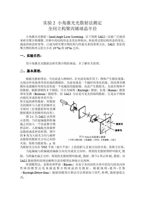
得到如下结论:1、球晶大小LLDPE/BR在室温冷却均能形成四叶瓣,但四叶瓣大小差别较大。
BR的加入改变了LLDPE球晶的大小:随着BR的增加体系的球晶出现由小到大变化的过程,当LLDPE/BR=60/40时,体系的球晶最大,球晶半径远大于纯LLDPE的球晶半径。
这是因为BR加入少时,即LLDPE/BR=90/10时,BR起到异相成核的作用,因而体系球晶有所较小;当BR增加时,妨碍了LLDPE分子链在结晶过程中的运动,因而形成的球晶变大。
2、结晶诱导期PP含量的改变对LLDPE/PP体系的结晶诱导期几乎没有影响,但对结晶温度敏感:在58℃等温结晶时,结晶诱导期为16秒;当结晶温度为85℃时,结晶诱导期变为20秒;98℃时为24秒,这是因为PP和LLDPE都为结晶型聚合物,而且结晶速率都较快,相对作为结晶驱动力的过冷度而言,LLDPE/PP用量的变化是微弱的;而与此同时,我们发现BR含量对LLDPE/BR体系的结晶诱导期影响较大,尤其是在较高结晶温度下时,随着BR含量的增加, LLDPE/PP体系的结晶诱导期明显缩短。
实验七小角激光光散射法测定全同立构聚丙烯球晶半径小角激光光散射(Small Angle Laser Scattering,以下简称SALS)法被广泛地用来研究聚合物薄膜、纤维中的结构形态及其拉伸取向、热处理过程结构形态的变化、液晶的相态转变等,已成为研究聚合物结构与性能关系的重要方法。
SALS表征的聚合物结构单元的大小在10-10m到10-8m之间。
一、实验目的:用小角激光光散射法研究聚合物的球晶,并了解有关原理。
二、基本原理:根据光散射理论,当光波进入物体时,在光波电场作用下,物体产生极化现象,出现由外电场诱导而形成的偶极矩。
光波电场是一个随时间变化的量,因而诱导偶极矩也就随时间变化而形成一个电磁波的辐射源,由此产生散射光。
光波在物体中的散射,根据谱频的3个频段,可分为瑞利(Rayleigh)散射,拉曼(Raman)散射和布里渊(Brillouin)散射等。
而SALS方法是可见光的瑞利散射。
它是由于物体内极化率或折射率的不均一性引起的弹性散射,即散射光的频率与入射光的频率完全相同(拉曼散射和布里渊散射都涉及到频率的改变)。
图7-1为SALS 法原理示意图。
当在起偏镜和检偏镜之间放入一个结晶聚合物样品时,入射偏振光将被样品散射成某种花样图。
图中的θ角为入射光方向与被样品散射的散射光方向之间的夹角,简称为散射角,μYOZ 平面(底片平面)上的投影与Z当起偏镜与检偏镜的偏振方向均为垂直方向时,得到的光散射图样叫做V V 散射,当两偏光镜正交时,得到的光散射图叫做V H 散射。
图7-1所示即V H 散射。
对SALS 散射图形的理论解释目前有模型法和统计法两种。
所谓模型法,是斯坦和罗兹(Rhodes )从处于各向同性介质中的均匀的各向异性球的模型出发来描述聚合物球晶的光散射,根据瑞利-德拜-甘斯(Rayleigh-Debye-Gans )散射的模型计算法可以得到如下的V V 和V H 散射强度公式:()()()()22033[2sin cos sin VV i s r s I AV a a U U U SiU a a SiU U U ⎛⎫=---+-- ⎪⎝⎭()()222cos cos 4sin cos 3]2r i a a U U U SiU θμ+-⨯-- ---------------(1)()()2222033[cos sin cos 4sin cos 3]2VH i r I AV a a U U U SiU U θμμ⎛⎫=-⨯-- ⎪⎝⎭(2)式中I 为散射光强度;V 0为球晶体积;i a 和r a 分别为球晶在切向和径向的极化率;s a 为环境介质的极化率;θ为散射角;μ为方位角;A 为比例常数。
小角x射线散射公式小角 X 射线散射(Small Angle X-ray Scattering,简称 SAXS)可是个相当有趣的话题呢!这其中涉及到的公式,那更是充满了奇妙的科学魅力。
咱们先来说说小角 X 射线散射到底是啥。
简单来讲,它就像是给物质内部结构拍了一张特殊的“照片”。
通过分析散射出来的 X 射线,我们就能了解物质内部的微观结构信息,比如孔隙大小、颗粒分布啥的。
那小角 X 射线散射公式到底长啥样呢?它通常可以表示为:I(q) =I₀ P(q) S(q) 。
这里的 q 是散射矢量,它跟入射 X 射线的波长、散射角度都有关系。
I₀呢,代表入射X 射线的强度。
就好比是灯光的亮度,灯光越亮,照亮的范围就越大。
P(q) 描述的是单个散射体的形状和大小相关的散射强度。
想象一下,不同形状和大小的物体,反射光线的情况是不是也不一样?这 P(q) 就是在说这个事儿。
S(q) 则是描述散射体之间相互关系的函数。
比如说一堆小球挤在一起,它们之间的距离、排列方式等等,都会影响散射的结果,S(q) 就是来处理这个的。
还记得我之前做过一个实验,那可真是让我对小角 X 射线散射公式有了更深刻的理解。
当时我们在研究一种新型的纳米材料,想要搞清楚它内部的孔隙结构。
为了得到准确的数据,我们在实验室里反复调试仪器,小心翼翼地控制着各种参数。
每次测量完数据,就开始对着小角 X 射线散射公式一顿琢磨。
有时候算出来的结果跟预期不太一样,就得重新检查数据,思考是不是哪个环节出了问题。
那感觉,就像是在解一道超级复杂的谜题,不过每一次有新的发现,都让人兴奋不已。
经过无数次的尝试和分析,终于利用这个公式成功地解析出了材料的孔隙结构。
那一刻,真的觉得所有的努力都值了!总之,小角 X 射线散射公式虽然看起来有点复杂,但只要我们深入去理解,多做实验,多分析数据,就能逐渐掌握它的奥秘,为我们探索物质的微观世界打开一扇神奇的大门。
所以呀,别被这公式吓到,勇敢地去探索,说不定你就能发现其中的无限乐趣和惊喜!。