Nonlinear dynamic characteristics of piles embedded in rock

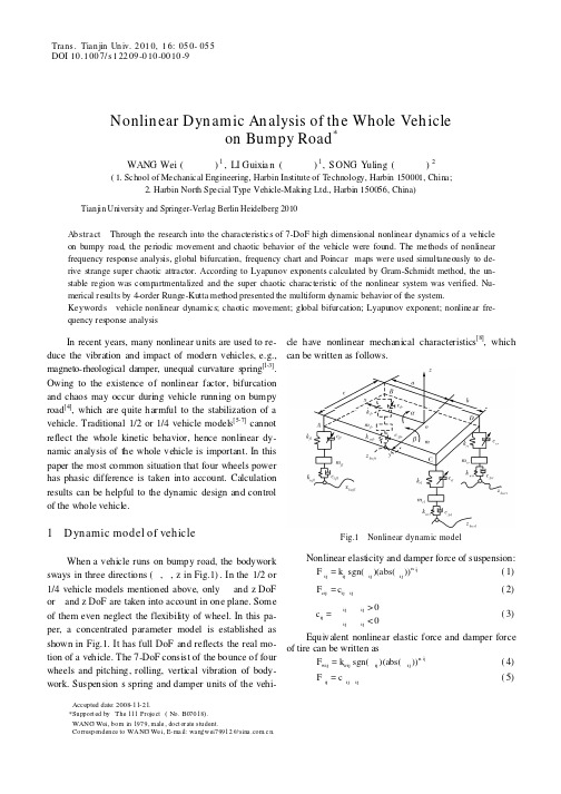
Trans.Tian jin Un iv.2010,16:050-055DOI 10.1007/s 12209-010-0010-9Accepted date:2008-11-21.*S y “T j ”(N B )W NG W ,,,W NG W ,@Nonlin ear Dyn amic An alysis of th e Whole Veh icleon Bumpy Road *WANG Wei (王威)1,LI Guixia n (李瑰贤)1,SONG Y uling (宋玉玲)2(1.School of Mechanical Engineering,Harbin Institute of Technology,Harbin 150001,China;2.Harbin North Special Type Vehicle-Making Ltd.,Harbin 150056,China)Tianjin University and Springer-Verlag Berlin Heidelberg 2010Ab stract ：Through the research into the characteristics of 7-DoF high dimensional nonlinear dynamics of a vehicle on bumpy road,the periodic movement and chaotic behavior of the vehicle were found.The methods of nonlinear frequency response analysis,global bifurcation,frequency chart and Poincar émaps were used simultaneously to de-rive strange super chaotic attractor.According to Lyapunov exponents calculated by Gram-Schmidt method,the un-stable region was compartmentalized and the super chaotic characteristic of the nonlinear system was verified.Nu-merical results by 4-order Runge-Kutta method presented the multiform dynamic behavior of the system.Keyword s ：vehicle nonlinear dynamics;chaotic movement;global bifurcation;Lyapunov exponent;nonlinear fre-quency response analysisIn recent years,many nonlinear units are used to re-duce the vibration and impact of modern vehicles,e.g.,magneto-rheological damper,unequal curvature spring [1-3].Owing to the existence of nonlinear factor,bifurcation and chaos may occur during vehicle running on bumpy road [4],which are quite harmful to the stabilization of a vehicle.Traditional 1/2or 1/4vehicle models [5-7]cannot reflect the whole kinetic behavior,hence nonlinear dy-namic analysis of the whole vehicle is important.In this paper the most common situation that four wheels power has phasic difference is taken into account.Calculation results can be helpful to the dynamic design and control of the whole vehicle.1Dynamic model of vehicleWhen a vehicle runs on bumpy road,the bodywork sways in three directions (α,β,z in Fig.1).In the 1/2or 1/4vehicle models mentioned above,only αand z DoF or βand z DoF are taken into account in one plane.Some of them even neglect the flexibility of wheel.In this pa-per,a concentrated parameter model is established as shown in Fig.1.It has full DoF and reflects the real mo-tion of a vehicle.The 7-DoF consist of the bounce of four wheels and pitching,rolling,vertical vibration of body-work.Suspension ’s spring and damper units of the vehi-cle have nonlinear mechanical characteristics [8],which can be written asfollows.Fig.1Nonlinear dynamic modelNonlinear elasticity and damper force of suspension:sgn()(abs())ijnij ij ij ijF k δδδδ=(1)ci j ij ijF c δ= (2)00ijij i j ij ijc δξδ>=< (3)Equivalent nonlinear elastic force and damper forceof tire can be written assgn()(abs())ijnwij wij i j ijF k ΔΔΔ=(4)ij ij ijF c ΔΔΔ= (5)upport ed b he 111Pro e ct o.07018.A ei born in 1979male doct orate student.Correspondence to A e i E-ma il:wa ngw .c n.WA NG W ei et al:Nonlinear Dynamic A nalysis of the Whole Vehicle on Bumpy Road—5—where i j k ,ij δand i j n δare equivalent stiffness coefficient,relative distortion and nonlinear coefficient of suspen-sion,respectively;i j c is suspension ’s equivalent damper coefficient;ij c Δis damper coefficient;wij k ,ijΔand ij n Δare equivalent spring stiffness coefficient,relative distortion and nonlinear coefficient of each tire,respectively;sgn()represents symbolic function;subscript i =(front,rear),j =(left,right).Through analyzing the kinetic model in Fig.1,the spring distortion can be obtained assin sin ij cwi j ij cw ij cwi j z z y x δδαβ′=+(6)Considering that H is the radius of wheel hub,thefollowing equation accounts for the elastic distortion of the tire:i j cwi jbwi jijz z H ΔΔ′=(7)where ij δ′and i jΔ′are static distortion ；cwij x ,cwij y and cwij z are centroid coordinates of wheel with cw ij x and cwij y being constant values.According to containing char-acteristic of road,its surface curve is supposed to have the following trigonometric function ：101()sin(2)2()sin(2)2bwrl rl bwrr rlrr a z t a ft A bz t b ft A B =+π+=+π++(8)where 0a and 0b are constant;rl A and rr B are phasic differ-ence between front wheel and rear wheel,left wheel and right wheel,respectively.Consequently,dynamic equa-tions can be described as,,,,()()ijcij i f r j l rfl cwfl fl cf l wfl f l fl fr cwf r fr cf rwf rfrfr rl cwrl rl crl w r l rl rl rr cw r r r r crr wrr rr rr x i jcij i f j l rmz mgFF m z F F F F m g m z F F F F m gm z F F F F m g m z F F F F m g J FF δδδδδδα==ΔΔΔΔ===+=+=+=+=+=+∑∑∑ ,,cos ()cos cwij r y ijcij cwi j i f rj l ry J FF x δαββ===+∑∑∑ (9)2Nonlinear frequency response analysisThe chaotic response may occur in an unstable areaof frequency,so the chaotic probability can be predicted through frequency analysis [9-11].The main parameters used in the numerical analysis are 1200m =kg,22i j m =kg,360x J =kg m 2,1600y J =kg m 2,ij k =22000N/m,5j =N ,5j ζ=N ,j ξ=N ,1.7, 1.7,ij i j n n δΔ== 1.2f l fr x x ==m,rl x =1.4rr x =m,fl y =0.8rl rr fr y y y ===m.Because the nonlinear dy-namic system is continuous,using 4-order Runge-Kutta method,the last calculated value of the previous step is regarded as the initial value for the next computation.Time interval is 1/100period and the total number of selected points is from 25000to 50000,which can avoid the influence of instantaneous response.For stable re-sponse,the absolute value of the maximum displacement is system output.Most scholars are interested in the part of resonance or low frequency response before the peak value of reso-nance,neglecting high frequency response after the peak value of resonance.In this paper,the chaotic behavior of a high speed vehicle is predicted in Fig.2.Displacement pow er parameters a re 0.1256r lA =rad,r rB =π/9ra d,110.05a b ==m,a 0/2=b 0/2=-0.5m.In Fig.2,thearrow-(a)Max rollingangle(b)Max pitchingangle(c)Max di s placementFig.2Results of frequency response analysisf f q y 120000wi k /m 200i s/m i 2000s/m head represents the direction o increasing re uenc .Transactions of Tianjin University V ol.16No.12010—5—Fig.2(a)shows that the discontinuous phenomenon of the curve is very frequent.It has intermittent and bounc-ing peculiarity.Unstable areas are mainly in frequency ranges of (10.2,10.4),(11.1,12.2)and (13.95,14.25).The discrete phenomenon also exists in Fig.2(b)and Fig.2(c).The unstable range that has evident jumping phenomenon is (13.95,14.25).The analysis mentioned above indicates that the most possible frequency area with chaotic motion is (13.95,14.25).When choosing f =14Hz,phase diagrams can be obtained as shown in Fig.3,which represent chaotic motion status in a small variable range of amplitude.A high speed vehicle can also produce chaotic vibration,but not evident.The fre-quency of the power is closely related to the velocity of vehicle,so unstable velocity area that may result in chaos should beavoided.(a)Rollingspeed(b)Pitchingspeed(c)Vertical speedFig.3Phase diagrams3Periodic m ovem ent,bifurcation and chaosConsidering the phasic difference A rl of front wheel and rear wheel as a bifurcation parameter,by printing Poincar époints,the displacement global bifurcation dia-gram can be obtained.Parameters rl A ∈[0.35,1.05],rr B =π/4r a d,11000.05m,/2/20.5m,a b a b f =====4.5Hz.Fig.4(a)and (b)have the same bifurcation charac-teristic.At bifurcation points,the system is unstable.The chaotic motion may occur in area (0.35,0.595)rl A ∈,while in other areas the system moves periodically.Further-more,the dynamic behavior of the system in idiographic bifurcation parameter area can be investigated by setting pa rameter s 0.65rl A =rad,4rr B =πrad,110.05m,a b ==00/2/20.5m a b ==, 4.5f =Hz,based on which Poin-car émapping of the system can be obtained,as shown in Fig.5.There are only three isolated points in Fig.5(a)and (b),so the systemic kinetic form is 1/3subharmonic periodic motion (3P).When 0.83r lA =rad,B rr =π/4rad,110.05a b ==m,0/2a =0/20.5m,b = 4.5f =Hz,an-other periodic motion form is also acquired.From Fig.6,16finite and isolated points exist individually in Fig.6(b)and (c).There should also be 16points in Fig.6(a)and (d),but some points are too close to be disting-wished.(a)Rollingangle(b)DisplacementF D f 2ig.4isplacement bi urcationWA NG W ei et al:Nonlinear Dynamic A nalysis of the Whole Vehicle on Bumpy Road—53—(a)Rollingspeed(b)Vertical speedFig.5Poincar émapping of system when A r l =0.65rad(a)Rollingspeed(b)Pitchingspeed(c)Verti calspeed(d)Wheel speedF 6éf y =3This shortcoming can be made up by time area analysis.Poincar émapping illuminates that the system moves periodically in the rough road.For the sake of making system kinetic status certain,frequency charts are computed as shown inFig.7.(a)Pit chingangle(b)Verti cal displacementFig.7Frequency chartThe power frequency 28.26ω=rad/s.To avoid fre-quency promiscuous phenomenon,the sampling period is1/500times the power frequency.From Fig.7,frequency v s peak value distributes in the same spacing and the spe-cific value between each other is a rational number.So the conclusion that the system moves periodically is proved.In Fig.7,the minimum frequency v s peak value is 1.776rad/s,which is 1/16times the power frequency.Fig.8shows that the vibration period of the system is 3.56s and it is 16times the power period.It is re-garded as a reason to explain why the system presents a 1/16subharmonic periodic motion.Similar analysis was carried out in area (0.86,0.88)r l A ∈and (0.88,1.05)r l A ∈.The result shows that the system presents 8P and 4P peri-odic motion,respectively.Chaos will occur if we choose parameters rl A =0.38ra d,/4rad,rr B =π110.05a b ==m,0/2a =0/20.5b =m,4.5f =Hz.According to calculation results of differen-tial equations in 10000power periods,the maximum displacement is treated as Poincar ésection,therefore Poincar émapping can be obtained.Poincar époints are ,ig.Poincar mapping o s stem when A rl 0.8radattracted to determinate area and represent strange char-Transactions of Tianjin University V ol.16No.12010—5—(a)Rollingangle(b)Wheel displacementFig.8Response vs timeacter.Frequency chart has continuous character and pre-sents backdrop and wide peak like noise.These phenom-ena are the symbol of chaos.The calculation results canbe obtained in Ref.[15].4Lyapunov exponen tsThe ultimate calculation result of Lyapunov expo-nent is the criterion to judge the chaotic behavior of sys-tem [12,13].The 14-dimensional non-autonomous dynamic system is turned into the 15-dimensional autonomousdynamic system before calculation.d (())d W x t W t =M f M x=0000(,)1(,)limln(,)t x x t x W t x t λ→∞Δ=Δ0(,0)0x x Δ→where W is the distance between two trajectories at time t;M is Jacobi or Lyapunov matrix;λis Lyapunov ex-ponent.When the vehicle dynamic system presents cha-otic behavior,considering the calculation course of Lyapunov exponents as a ball evolutive process,the dis-tance between two trajectories changes according to ex-ponential rule,at the same time the distortion of ball changes according to the same rule.To ensure the direc-tion coherence of vector,Gram-Schmidt method [14]is applied in this paper.The computation flow chart is shown in Fig.9.According to Fig.9,the simulation time is 5000s,the result can be acquired as shown in Ref.[15],which is consistent with the kinetic status of the system.When two values of Lyapunov exponents are bigger than zero,the system has super-chaotic character,so the attractor is super-chaotic.When the system moves periodically (3P),only one Lyapunov exponent is equal to zero,the others are smaller than zero,it can be concluded that the kinetic modality of the system is a limit cycle.The circs of 4P,8P and 16P is similar to that of 3P.We can also derive the convergent and emanative status of eachdimension.Fig.9Computation flow chart of Lyapunov exponents4WA NG W ei et al:Nonlinear Dynamic A nalysis of the Whole Vehicle on Bumpy Road—55—5ConclusionsThe chaotic vibration course of vehicle dynamic sys-tem is converse double period bifurcation (4P,8P,16P)to 1/3sub-harmonic wave period movement,finally to chaotic vibration.The unstable area of vehicle speed can be predicted by the analysis of frequency response,which can be used to control the speed of vehicle under the con-dition of certain road.By the analysis of global bifurca-tion and Lyapunov exponents,the stable and unstable areas of system are calculated for the dynamic control and design of vehicle.Refer ences［1］Lai C Y ,Liao W H.Vibration control of a suspension sys-tem via magneto-rheological fluid damper[J].Journal of V ibration and Control,2002,8(4):515-527.［2］Choi S B,Lee S K.A hysteresis model for the field-dependent damping force of amagneto-rheologicaldamper[J].Journal of Sound and V ibration,2001,24:361-375.［3］Liu H,Nonami K,Hagiwara T.Semi-active fuzzy slidingmode control of full vehicle and suspensions [J].Journal of V ibration and Control,2005,11(8):1025-1042.［4］Litak G,Borowiec M,Friswell M I et al.Chaotic vibrationof a quarter-car model excited by the road surface pro-file[EB/OL].Commun Nonlinear Sci Numer Simul,2007,doi:10.1016/sns.2007.01.003.［5］Campos J,Davis L,Lewis F L et al.Active suspensioncontrol of ground vehicle heave and pitch motions[C].In:Proceedings of the 7th IEEE Mediterranean Control Con-ference on Control and Automation.Haifa,Israel,1999.222-233.［6］Williams R A.Automotive active suspensions (Part 1):Basic principles[J].Proceedings of the Institution of Me-chanical Engineers,Part D:Journal of Automobile Engi-neering,1997,211(6):415-426.［7］Szabelski K.The vibrations of self-excited system withparametric excitation and non-symmetric elasticity charac-teristics[J].J Theor Appl Mech,1991,29:57-81.［8］Moran A,Nagai M.Optimal active control of nonlinearvehicle suspensions using neural networks[J].JSME In-ternational Journal,Series C,1994,37(4):707-718.［9］Belato D,Weber H I,Balthazar J M et al.Chaotic vibrationof a non-ideal electro-mechanical system[J].International Journal of Solids and Structures,2001,38:1699-1706.［10］Zhu Q,Tani J,Takagi T.Chaotic vibrations of a magneti-cally levitated system with two degrees of freedom[J].Journal of T echnical Physics,1994,35(1/2):171-184.［11］Pust L,Sz ll s O.The forced chaotic and irregular oscilla-tions of the nonlinear two degrees of freedom system[J].International Journal of Bifurcation and Chaos in Applied Sciences and Engineering,1999,9(3):479-491.［12］Hoover W G ,Hoover C G,Grond F.Phase-space growthrates,local Lyapunov spectra and symmetry breaking for time-reversible dissipative oscillators[J].Communications in Nonlinear Science and Numerical Simulation,2008,13(6):1180-1193.［13］Zhang J G .Hopf bifurcations,Lyapunov exponents andcontrol of chaos for a class of centrifugal fly wheel gover-nor system[EB/OL].Chaos,Solitons and Fractals,2007,doi:10.1016/j.chaos.2007.06.131.［14］Parker T S,Chua L O.Numerical A lgorithms for ChaoticSystem[M].Springer Verlag,New York,1989.［15］W ang Wei,Li Guixian,Song Yuling.Study on super cha-otic vibration of whole vehicle dynamic model via time-delay power of four wheels[J].V ibration and Shock,2009,28(3):102-106(in Chinese).。

1/4波片quarter-wave plateCG矢量耦合系数Clebsch-Gordan vector coupling coefficient; 简称“CG[矢耦]系数”。

X射线摄谱仪X-ray spectrographX射线衍射X-ray diffractionX射线衍射仪X-ray diffractometer[玻耳兹曼]H定理[Boltzmann] H-theorem[玻耳兹曼]H函数[Boltzmann] H-function[彻]体力body force[冲]击波shock wave[冲]击波前shock front[狄拉克]δ函数[Dirac] δ-function[第二类]拉格朗日方程Lagrange equation[电]极化强度[electric] polarization[反射]镜mirror[光]谱线spectral line[光]谱仪spectrometer[光]照度illuminance[光学]测角计[optical] goniometer[核]同质异能素[nuclear] isomer[化学]平衡常量[chemical] equilibrium constant[基]元电荷elementary charge[激光]散斑speckle[吉布斯]相律[Gibbs] phase rule[可]变形体deformable body[克劳修斯-]克拉珀龙方程[Clausius-] Clapeyron equation[量子]态[quantum] state[麦克斯韦-]玻耳兹曼分布[Maxwell-]Boltzmann distribution[麦克斯韦-]玻耳兹曼统计法[Maxwell-]Boltzmann statistics[普适]气体常量[universal] gas constant[气]泡室bubble chamber[热]对流[heat] convection[热力学]过程[thermodynamic] process[热力学]力[thermodynamic] force[热力学]流[thermodynamic] flux[热力学]循环[thermodynamic] cycle[事件]间隔interval of events[微观粒子]全同性原理identity principle [of microparticles][物]态参量state parameter, state property[相]互作用interaction[相]互作用绘景interaction picture[相]互作用能interaction energy[旋光]糖量计saccharimeter[指]北极north pole, N pole[指]南极south pole, S pole[主]光轴[principal] optical axis[转动]瞬心instantaneous centre [of rotation][转动]瞬轴instantaneous axis [of rotation]t 分布student's t distributiont 检验student's t testＫ俘获K-captureＳ矩阵S-matrixＷＫＢ近似WKB approximationＸ射线X-rayΓ空间Γ-spaceα粒子α-particleα射线α-rayα衰变α-decayβ射线β-rayβ衰变β-decayγ矩阵γ-matrixγ射线γ-rayγ衰变γ-decayλ相变λ-transitionμ空间μ-spaceχ 分布chi square distributionχ 检验chi square test阿贝不变量Abbe invariant阿贝成象原理Abbe principle of image formation阿贝折射计Abbe refractometer阿贝正弦条件Abbe sine condition阿伏伽德罗常量Avogadro constant阿伏伽德罗定律Avogadro law阿基米德原理Archimedes principle阿特伍德机Atwood machine艾里斑Airy disk爱因斯坦-斯莫卢霍夫斯基理论Einstein-Smoluchowski theory 爱因斯坦场方程Einstein field equation爱因斯坦等效原理Einstein equivalence principle爱因斯坦关系Einstein relation爱因斯坦求和约定Einstein summation convention爱因斯坦同步Einstein synchronization爱因斯坦系数Einstein coefficient安[培]匝数ampere-turns安培[分子电流]假说Ampere hypothesis安培定律Ampere law安培环路定理Ampere circuital theorem安培计ammeter安培力Ampere force安培天平Ampere balance昂萨格倒易关系Onsager reciprocal relation凹面光栅concave grating凹面镜concave mirror凹透镜concave lens奥温电桥Owen bridge巴比涅补偿器Babinet compensator巴耳末系Balmer series白光white light摆pendulum板极plate伴线satellite line半波片halfwave plate半波损失half-wave loss半波天线half-wave antenna半导体semiconductor半导体激光器semiconductor laser半衰期half life period半透[明]膜semi-transparent film半影penumbra半周期带half-period zone傍轴近似paraxial approximation傍轴区paraxial region傍轴条件paraxial condition薄膜干涉film interference薄膜光学film optics薄透镜thin lens保守力conservative force保守系conservative system饱和saturation饱和磁化强度saturation magnetization本底background本体瞬心迹polhode本影umbra本征函数eigenfunction本征频率eigenfrequency本征矢[量] eigenvector本征振荡eigen oscillation本征振动eigenvibration本征值eigenvalue本征值方程eigenvalue equation比长仪comparator比荷specific charge; 又称“荷质比(charge-mass ratio)”。

Nonlinear Systems and Control Nonlinear systems and control are essential topics in the field of engineering and mathematics. These systems are characterized by their complex behavior, which cannot be fully described by linear equations. Nonlinear systems can exhibit awide range of behaviors, including chaos, bifurcation, and instability, making them challenging to analyze and control. One of the key challenges in dealingwith nonlinear systems is the lack of a general theory that can be applied to all such systems. Unlike linear systems, which can be analyzed using well-established techniques such as Laplace transforms and transfer functions, nonlinear systems require more sophisticated methods, such as Lyapunov stability analysis, phase plane analysis, and numerical simulations. These methods often require a deep understanding of the underlying mathematics and can be computationally intensive, making the analysis and control of nonlinear systems a daunting task. Another challenge in dealing with nonlinear systems is the presence of uncertainties and disturbances. In real-world applications, nonlinear systems are often subject to external disturbances and uncertainties in the system parameters, which can significantly affect their behavior. This makes it difficult to design controllers that can effectively stabilize and control the system in the presence of such uncertainties. Robust control techniques, such as H-infinity control and sliding mode control, have been developed to address these challenges, but they often require a detailed knowledge of the system dynamics and uncertainties, which may not always be available. Nonlinear systems also pose challenges in terms of their control and optimization. Unlike linear systems, where the optimal control and optimization problems can often be solved analytically, nonlinear systems require the use of numerical optimization techniques, such as gradient descent and genetic algorithms. These methods can be computationally expensive and may not always guarantee convergence to the global optimum, especially for highly nonlinear and complex systems. Despite these challenges, the study of nonlinear systems and control is of great importance in many engineering and scientific disciplines. Nonlinear systems are ubiquitous in nature, appearing in fields such as physics, biology, and economics. Understanding and controlling these systems is essentialfor developing advanced technologies, such as autonomous vehicles, robotic systems,and renewable energy systems, which often exhibit highly nonlinear behavior. In conclusion, the analysis and control of nonlinear systems pose significant challenges due to their complex behavior, uncertainties, and the lack of a general theory. However, the study of nonlinear systems is crucial for advancing technology and understanding natural phenomena. Researchers and engineers continue to develop new methods and techniques to address these challenges, with the goal of effectively analyzing and controlling nonlinear systems in a wide range of applications.。

土木工程专业裂缝宽度容许值: allowable value of crack width使最优化: optimized次最优化: suboptimization主梁截面: girder section主梁: girder|main beam|king post桥主梁: bridge girder单墩: single pier结构优化设计: optimal structure designing多跨连续梁: continuous beam on many supports裂缝crackcrevice刚构桥: rigid frame bridge刚度比: ratio of rigidity|stiffness ratio等截面粱: uniform beam|uniform cross-section beam 桥梁工程: bridgeworks|LUSAS FEA|Bridge Engineering桥梁工程师: Bridge SE预应力混凝土: prestressed concrete|prestre edconcrete 预应力混凝土梁: prestressed concrete beam预应力混凝土管: prestressed concrete pipe最小配筋率minimum steel ratio轴向拉力, 轴向拉伸: axial tension英语重点词汇承台: bearing platform|cushioncap|pile caps桩承台: pile cap|platformonpiles低桩承台: low pile cap拱桥: hump bridge|arch bridge|arched bridge强度: intensity|Strength|Density刚强度: stiffness|stiffne|westbank stiffness箍筋: stirrup|reinforcement stirrup|hooping预应力元件: prestressed element等效荷载: equivalent load等效荷载原理: principle of equivalent loads模型matrixmodelmouldpattern承载能力极限状态: ultimate limit states正常使用极限状态: serviceability limit state 弹性: elasticity|Flexibility|stretch平截面假定: plane cross-section assumption抗拉强度intensity of tensiontensile strength安全系数safety factor标准值: standard value,|reference value作用标准值: characteristic value of an action重力标准值: gravity standard设计值: design value|value|designed value作用设计值: design value of an action荷载设计值: design value of a load可靠度: Reliability|degree of reliability不可靠度: Unreliability高可靠度: High Reliability几何特征: geometrical characteristic塑性plastic natureplasticity应力图: stress diagram|stress pattern压应力: compressive stress|compression stress配筋率: reinforcement ratio纵向配筋率: longitudinal steel ratio有限元分析: FEA|finite element analysis (FEA)|ABAQUS有限元法: finite element method线性有限元法: Linear Finite Element Method裂缝控制: crack control控制裂缝钢筋: crack-control reinforcement应力集中: stress concentration主拉应力: principal tensile stress非线性nonlinearity非线性振动: nonlinear vibration弯矩: bending moment|flexural moment|kN-m弯矩图: bending moment diagram|moment curve弯矩中心: center of moments|momentcenter剪力: shearing force|shear force|shear剪力墙: shear wall|shearing wall|shear panel弹性模量elasticity modulus剪力图: shear diagram|shearing force diagram剪力和弯矩图: Shear and Moment Diagrams剪力墙结构: shear wall structure轴力: shaft force|axial force框架结构frame construction板单元: plate unit曲率curvature材料力学mechanics of materials结构力学: Structural Mechanics|theory of structures 弯曲刚度: bending stiffness|flexural rigidity截面弯曲刚度: flexural rigidity of section弯曲刚度，抗弯劲度: bending stiffness钢管混凝土结构: encased structures极限荷载: ultimate load极限荷载设计: limit load design|ultimate load design 板壳力学: Plate Mechanic主钢筋: main reinforcement|Main Reinforcing Steel 钢筋混凝土的主钢筋: main bar悬臂梁: cantilever beam|cantilever|outrigger悬链线: Catenary,|catenary wire|chainetteribbed stiffener加劲肋: stiffening rib|stiffener|ribbed stiffener短加劲肋: short stiffener支承加劲肋: bearing stiffener技术标准technology standard水文: Hydrology招标invite public bidding连续梁: continuous beam|through beam多跨连续梁: continuous beam on many supports wind resistance抗风: Withstand Wind |wind resistance基础的basal初步设计predesignpreliminary plan技术设计: technical design|technical project施工图设计: construction documents design基础foundationbasebasis 结构形式: Type of construction|form of structure屋顶结构形式: roof form地震earthquake地震活动: Seismic activity|seismic motion耐久性: durability|permanence|endurance耐久性试验: endurance test|life test|durability test短暂状况: transient situation偶然状况: accidental situation永久作用: permanent action永久作用标准值: characteristic value of permanent action可变作用: variable action可变作用标准值: characteristic value of variable action可变光阑作用: iris action偶然作用: accidental action作用效应偶然组合: accidental combination for action effects作用代表值: representative value of an action作用标准值: characteristic value of an action地震作用标准值: characteristic value of earthquake action可变作用标准值: characteristic value of variable action作用频遇值Frequent value of an action安全等级: safety class|Security Level|safeclass设计基准期: design reference period作用效应: effects of actions|effect of an action作用效应设计值Design value of an action effect分项系数: partial safety factor|partial factor作用分项系数: partial safety factor for action抗力分项系数: partial safety factor for resistance作用效应组合: combination for action effects结构重要性系数Coefficient for importance of a structure桥涵桥涵跟桥梁比较类似，主要区别在于:单孔跨径小于5m或多孔跨径之和小于8m的为桥涵,大于这个标准的为桥梁水力: hydraulic power|water power|water stress跨度span人行道sidewalk无压力: stress-free净高clear height矩形rectangle无铰拱: arch without articulation|fixed end arch荷载load荷载强度: loading intensity|loading inte ity荷载系数: load factor|loading coefficient桥头堡bridgeheadbridge tower美观pleasing to the eyebeautifulartistic经济的economicaloecumenicaleconomic适用be applicable防水waterproof剪切模量: shear modulus|rigidity modulus|GXY剪切强度: shear strength|shearing strength|Fe-Fe扭转剪切强度: torsional shear strength剪切破坏: shear failure|shear fracture|shear damage 纯剪切破坏: complete shear failure局部剪切破坏: local shear failure永久冻土: permafrost|perennial frost土的侧压力: earth lateral pressure收缩shrinkpull backcontract徐变: creep摩擦系数: coefficient of friction|friction factor风荷载: wind load|wind loading风荷载标准值: characteristi cvalue of windload 风荷载体型系数: shape factor of windload温度作用: temperature action支座: support|bearing|carrier 外支座: outer support|outersu ort代表值: central value|representative value结构自重: self-weightstructure|dead load最不利分布: Least favorable distribution,抗震antiknockquake-proofearthquake proofing constructionearthquake-resistanceearthquake proof钢结构steel structure钢结构设计: Design Of Steel Structure钢结构设计规范: Code for design of steel structures 混凝土结构设计规范: Code for design of concrete structures预应力混凝土结构设计软件: PREC温度梯度: temperature gradient|thermal gradient动力系数: dynamic coefficient制动力系数: Braking force coefficient动力学kineticsdynamicsdyn内摩擦角: angle of internal friction有效内摩擦角: effective angle of internal friction主效应main effect主效应: Main effect,主效应模型: Main effect model超静定的: hyperstatic超静定结构: statically indeterminate structure静定: statically determinate静定梁: statically determinate beam附属设备: accessories|accessory equipment稳定系数: coefficient of stabilizationearth pressure at rest静土压力: earthpressureatrest挡土墙retaining wallabamurus主动土压力: active earth pressure被动土压力: passive earth pressure土层soil horizon土层剖面: soil profile土层剖面特性: soil-profile characteristics密度densitythickness宽度width净距: clear distance|gabarit|Clearance钢筋强度标准值: characteristic value of strength of steel bar钢材强度标准值: characteristic value of strength of steel折减系数: reduction factor|discount coefficient强度折减系数: strength reduction factor线性linearity线性代数linear algebra位移displacement位移角: angle of displacement|angle of slip应变量: dependent variable|strain capacityuniform stress均布应力: uniform stress非均布应力: non-uniform stress均布荷载: uniformly distributed load集中荷载: concentrated load|point load可变集中荷载: variable concentrated load法向集中荷载: normal point load影响线: influence line反力影响线: influence line for reaction影响线方程: equation of the influence line车辆荷载: car load|vehicular load|traffic load计算跨径: calculated span重力加速度: acceleration of gravity膨胀系数: coefficient of expansion|expansivity术语termterminology恒载: dead load|deadloading|permanent load活载: live load楼面活载: floor live load概率分布: probability distribution 联合概率分布: Joint probability distribution,边缘概率分布: Marginal probability distribution,拱腹: soffit|intrados|arch soffit三铰拱: three hinged arch土木工程系: Department of Civil Engineering土木工程师协会: ICE土木工程师协会: Institute of Civil Engineers作用准永久值: quasi－permanentvalueofanaction 直径diameter验算: checking|check calculation验算公式: check formula变形验算: deformation analysis建筑材料tignum刚度rigidityseveritystiffness单元: cell|Unit|module节点node位移方程式: strain displacement equation三维three dimensional 3d插值: Interpolation|interpolate|Spline插值法: interpolation|method of interpolation轴对称axial symmetryrotational symetryaxisymmetric(al)应变矩阵strain matrix应变矩阵: strain matrix单元应变矩阵: element strain matrix应力应变矩阵: stress-strainmatrix阻尼矩阵: damping matrix|daraf|damped matrix 弹性系数矩阵: elastic coefficient matrix雅可比矩阵: Jacobi matrix|jacobian matrix刚度矩阵: stiffness matrix|rigidity matrix质量矩阵: mass matrix|ma matrix节点力: nodal forces等效节点力: equivalent nodal force节点荷载: joint load|nodal loads节点荷载: joint load|nodal loads一致节点荷载: consistent nodal load应力矩阵: stress matrix挠度: deflection|flexivity|flexure转角: corners|intersection angle|rotor angle单元刚度矩阵: element stiffness matrix边界条件: boundary condition|edge conditions疲劳强度: fatigue strength|endurance strength抗疲劳强度: fatigue resistance工程局: construction bureau沉井基础: open caisson foundation水泥cement水泥砂浆cement mortar石膏: Gypsum|plaster|Plaster of Paris简支梁: simply supported beam|simple beam简支梁桥: simple supported girder bridge平衡条件: equilibrium condition|balance condition约束条件: constraint condition|constraint数值解: numerical solution|arithmeticsolution力法: force method|brute force method位移法: displacement method|di lacement method力矩分配法: moment distribution method|moment diagram理论力学: Theoretical Mechanics弹性力学: Theory of Elastic Mechanics结构动力学: Structural Dynamics|Clough高等结构动力学: Advancd Dynamics of Structures测量学: surveying|metrology|geodesy道路工程: road works|highway construction铁路工程: railway engineering|rairoad engineering隧道: Tunnels|subway|underpass轨道: orbit|track|trajectory砂子: sand抗压强度pressive strength焊接技术: Welding Engineering Technology (WET)断裂力学: Fracture Mechanics|fracturing mechanics基础工程: foundation engineering|foundation works 地质学: geology|die Geologie, opl.|geognosy岩土力学: rock mechanics|rock-soil mechanics工程力学: engineering mechanics轴线axes拱脚: arch springing|abutment|spring木桥: timber bridge|wodden bridge|Woodbridge枕木sleeper crosstie残余应力: residual stress|remaining stress 复合应力: combined stress|compound stress初始应力: initial stress|primary stress屈服极限: yield limit|minimum yield|yield strength疲劳屈服极限: fatigue yield limit应力幅值: stress amplitude冲击韧性: impact toughness|Impelling strength反弯点: knick point|pointofcontraflexure桁架: truss|tru|Girder网架结构: space truss structure|grid structure锚孔: anchor eye大跨度: High-span柱: column|pillar|Clmn. Coloumn常微分方程: Ordinary Differentical Equations|ODE|ODEs增大系数: enhancementcoefficient浮桥flying bridge raft bridgepontoon bridge pontoonfloat bridge浮桥: pontoon bridge|pontoon|floating bridge轮渡: Ferry|Ferries|ferry boat钢桥: steel bridge立面图: elevation|elevation drawing|profile背立面图: back elevation平面图: plan|plan view|planar graph泥石流: debris flow|rollsteinfluten|mud-rock flow大型泥石流: macrosolifluction滑坡泥石流: landslide模板: template|die plate, front board|formwork沉降: settlement|sedimentation|subside沉降缝: settlement joint伸缩缝: expansion joint路灯street lamp排水系统: drainage system|sewerage system泄水管: drain pipe|Scupper Pipe|tap pipe土力学: soil mechanics|Bodenmechanik高等土力学: Advanced Soil Mechanics扩展(扩大)基础: spread foundation桩基础: pile foundation|pile footing|Pile砂桩基础: sand pile foundation群桩基础: multi-column pier foundation沉箱基础caisson foundation沉箱基础: caisson foundation|laying foundation管状沉箱基础: cylinder caisson foundation气压沉箱基础: pneumatic caisson foundation桩承台: pile cap|platformonpiles桩: pile|pile group|pale灌注桩: cast-in-place pile|cast in place管灌注桩: driven cast-in-place pile灌注混凝土基础: cast-in-place concrete foundation 承台结构: suspended deck structure工作机理working mechanism铆钉: rivet|rivet riv|clinch bolt卵石: cobble|gravel|pebble钢筋混凝土结构: reinforced concrete structure预应力混凝土结构: prestressed concrete structure软化: softening|mollification|malacia强化: reinforcement|consolidate|intensification固体力学: solid mechanics|механика твердого тела 虚功原理: principle of virtual work偏心距: eccentricity|throw of eccentric偏心距增大系数: amplified coefficient of eccentricity 强度准则: strength criterion变形: Deformation|Transforms|deform工程建设: engineering construction石油工程建设: Petroleum Engineering Construction 偏心受压: eccentric compression偏心受压构件: eccentric compression member弹性支承: elastomeric bearing|yielding support temperature load温度荷载: temperature load施工控制: construction control经纬仪theodolite transit instrument夹具jig tongs clamp切线: tangent|Tangent line,|tangential line水平角: horizontal angle|inclination高程index elevation height altitude沼泽marsh swamp glade水准仪water level公寓apartment砂浆mortar sand pulp骨料skeletal material aggregate骨料级配: aggregate grading|aggregate gradation碱性的: alkalic|basic|alkalescent耐碱性的: alkali-proof风洞试验: wind tunnel test先张法: pre-tensioning|pretensioning method配合比设计: mix design|design of mix proportion 和易性: workability渗透性osmosis penetrability水泥浆: grout|cement slurry|cement paste对称的symmetrical symmetric(al)扭转reverseturn around (an undesirable situation)扭转应力: torsion stress|warping stress容许扭转应力: allowable twisting stress扭转角: angle of torsion|angle of twist夯实回填土: tamped backfill|tamped/compacted backfill圆锥贯入仪: cone penetrometer水化（作用）: hydration水化热: heat of hydration|heat of hydratation振捣器: vibrating tamper|vibrorammer|vibrator板振捣器: slab vibrator破裂fracture burst结合力: binding force|Adhesion|cohesion碎石gravel gravely脆性brittleness脆性材料: brittleness material|brittle material脆性破坏: brittle failure|brittle fracture素混凝土: plain concrete素混凝土结构: plain concrete construction含水量liquid water content钢筋: Reinforcement|bar tendon主钢筋: main reinforcement|Main Reinforcing Steel钢筋条: reinforcement bar|steel bar极限抗拉应力: ultimate tensile strength极限抗拉强度: ultimate tensile strength|UTS混凝土板: concrete slab预制混凝土板: precast concrete plank锚固: anchoring|anchorage|Anchor锚具: anchorage|anchorage device|ground tackle削弱weaken埋置: embedding|elutriator|imbedment预应力钢筋: prestressed reinforcement回弹: resilience|spring back|rebound有说服力的: persuasive|convincing|convictive形心centre of figurecentre of formcentroid重心center of gravity(n) core; main part惯性矩: moment of inertia极惯性矩: polar moment of inertia质心centroid center of mass回转半径: radius of gyration|turning radius容许应力: allowable stress|permissible stress排架: shelving|bent frame|bent桩排架: pile bent纵梁longeron carling横梁: beam|cross beam|transverse beam缆索cable thick rope阻尼damping刚架: rigid frame|frame|stiffframe缀板batten plate缀板: batten plate|stay plate|batte latebatten plate缀板: batten plate|stay plate|batte late上部缀板: upper stay plate推力: thrust|Push|Push Power槽钢channel steel特征值: Eigenvalue,|characteristic value冷拔钢丝: cold drawn wire自振频率: natural frequency of vibration自振周期: natural period of vibration土壤加固工程: soil stabilization works结构加固工程: structural fortification应力分析: stress analysis|stress distribution结构分析: structural analysis|ETABS NL结构稳定性: structural stability结构工程: Structural Engineering|structural works 认可标准: recognized standard|approved standard 官方认可标准: officially recognized standard,再循环: recycle|recirculation|recycling快硬水泥: rapid hardening cement|ferrocrete曲率半径: radius of curvature|curve radius|ρ刚性系数: coefficient of rigidity乡郊地区: rural area饱和saturation饱和密度: saturated density|Saturation density脚手架staging scaffold falsework立体剖面图: sectional axonometric drawing结构控制: structural control收缩量: Shrinkage|amount of shrinkage间距space between 钢管steel tube工字钢桩: steel H pile钢绞线: Steel Strand|Steel Stranded Wire|strand群震: swarm earthquake系统误差: systematic error|fixed error|system error最大剪应力: maximum shear|maximum shearing stress最大剪应变: maximum shear strain千斤顶: jack|lifting jack|Wheeljack地震系数: seismic coefficient|seismic factor。

附录A英文原文Experimental and Numerica Studies on Nonlinear Dynam Behavior of Rotor System Supported by Ball BearingsBall bearings are important mechanical components in high-speed turbomachinery that is liable for severe vibration and noise due to the inherent nonlinearity of ball ing experiments and the numerical approach, the nonlinear dynamic behavior of a flexible rotor supported by ball bearings is investigated in this paper. An experimental ball bearing-rotor test rig is presented in order to investigate the nonlinear dynamic performance of the rotor systems, as the speed is beyond the first synchroresonance frequency. The finite element method and two-degree-of-freedom dynamic model of a ball bearing are employed for modeling the flexible rotor s ystem. The discrete model of a shaft is built with the aid of the finite element technique, and the ball bearing model includes the nonlinear effects of the Hertzian contact force, bearing internal clearance, and so on.The nonlinear unbalance response is observed by experimental and numerical analysis.All of the predicted results are in good agreement with experimental data, thus validating the proposed model. Numerical and experimental results show that the resonance frequency is provoked when the speed is about twice the synchroresonance frequency, while the subharmonic resonance occurs due to the nonlinearity of ball bearings and causes severe vibration and strong noise. The results show that the effect of a ball bearing on the dynamic behavior is noticeable in optimum design and failure diagnosis of high-speed turbomachinery. [DOI: 10.1115/1.4000586]Keywords: ball bearing, rotor, experiment, nonlinear vibrationA.1 IntroductionBall bearings are one of the essential and important components in sophisticated turbomachinery such as rocket turbopumps, aircraft jet engines, and so on. Because of the requirement of acquiring higher performance in the design and operation of ballbearings-rotor systems, accurate predictions of vibration characteristics of the systems, especially in the high rotational speed condition, have become increasingly important.Inherent nonlinearity of ball bearings is due to Hertzian contact forces and the internal clearance between the ball and the ring.Many researchers have devoted themselves to investigating the dynamiccharacteristics associated with ball bearings. Gustafsson et al. [1] studied the vibrations due to the varying compliance of ball bearings. Saito [2] investigated the effect of radial clearance in an unbalanced Jeffcott rotor supported by ball bearings using the numerical harmonic balance technique. Aktürk et al. [2] used a three-degree-of-freedom system to explore the radial and axial vibrations of a rigid shaft supported by a pair of angular contact ball bearings. Liew et al. [4] summarized four different dynamic models of ball bearings, viz., two or five degrees of freedom, with or without ball centrifugal force, which could be applied to determine the vibration response of ball bearing-rotor systems. Bai and Xu [5] presented a general dynamic model to predict dynamic properties of rotor systems supported by ball bearings. De Mul et al. [6] presented a five-degree-of-freedom (5DOF) model for the calculation of the equilibrium and associated load distribution in ball bearings. Mevel and Guyader [7] described different routes to chaos by varying a control parameter. Jang and Jeong [8] proposed an excitation model of ball bearing waviness to investigate the bearing vibration. Then, considering the centrifugal force and gyroscopic moment of ball, they developed an analytical method to calculate the characteristics of the ball bearing under the effect of waviness in Ref. [9]. Tiwari et al. [10,11] employed a two-degree-of-freedom model to analyze the nonlinear behaviors and stability associated with the internal clearance of a ball bearing.Harsha [12-14], taking into account different sources of nonlin-earity, investigated the nonlinear dynamic behavior of ball bearing-rotor systems. Gupta et al. [15] studied the nonlinear dynamic response of an unbalanced horizontal flexible rotor supported by a ball bearing. With the aid of the Floquet theory, Bai et al. [16] investigated the effects of axial preload on nonlinear dynamic characteristics of a flexible rotor supported by angular contact ball bearings. Using the harmonic balance method, Sinou [17]performed a numerical analysis to investigate the nonlinear unbalance response of a flexible rotor supported by ball bearings.In the abovementioned studies, main attention has been paid to the ball bearing modeling and the dynamic properties analysis according to simple bearing-rotor models. With theoretical analysis and experiment, Yamamoto et al. [18] studied a nonlinear forced oscillation at a major critical speed in a rotating shaft,which was supported by ball bearings with angular clearances.Ishida and Yamamoto [19] studied the forced oscillations of a rotating shaft with nonlinear spring characteristics and internal damping. They found that a self-excited oscillation appears in the wide range above the major critical speed. A dynamic model was derived, and experiments are carried out with a laboratory test rig for studying the misaligned effect of misaligned rotor-ball bearing systems in Ref. [20]. Tiwari et al. [21] presented an experimental analysis to study the effect of radial internal clearance of a ball bearing on the bearingstiffness of a rigid horizontal rotor. These experimental results validated theoretical results reported in their literatures [10,11]. Recently, Ishida et al. [22] investigated theoretically and experimentally the nonlinear forced vibrations and parametrically excited vibrations of an asymmetrical shaft supported by ball bearings. Mevel and Guyader [23] used an experimental test bench to confirm the predicted routes to chaos in their previous paper [7]. It is noticeable of lack of experiments on nonlinear dynamic behavior of flexible rotor systems supported by ball bearings. In Ref. [24], the finite element method was used to model a LH2 turbopump rotor system supported by ball bearings. Numerical results show that the subharmonic resonance, as well as synchroresonance, occurs in the start-up process. It is found that the subharmonic resonance is an important dynamic behavior and should be considered in engineering ball bearing-rotor system design. But, the experimental and numerical studies of the subharmonic resonance in ball bearing-rotor systems are very rare.With respect to the above, the present study is intended to cast light on the subharmonic resonance characteristics in ball bearing-rotor systems using experiments and numerical approach. An experiment on an offset-disk rotor supported by ball bearings is carried out, and the finite element method and two-degree-of-freedom model of a ball bearing are employed for modeling this rotor system. The predicted results are compared with the test data, and an investigation is conducted in the nonlinear dynamic behavior of the ball bearings-rotor system.2 Experimental InvestigationAn experimental rig is employed for studying the nonlinear dynamic behavior of ball bearing-rotor systems, as shown in Fig.1. The horizontal shaft is supported by two ball bearings at both ends, and the diskis mounted unsymmetrically. The shaft is coupled to a motor with a flexible coupling. The motor speed is controlled with a feedback controller, which gets the signals from an eddy current probe. Four eddy current probes, whose resolution is 0.5 m, are mounted close to the disk and bearing at the right end in the horizontal and vertical directions, respectively. The displacement signals, obtained with the help of probes, are input into an oscilloscope to describe the motion orbit, and a data acquisition and processing system were used to analyze the effects of ball bearings on the nonlinear dynamic behavior. The data acquisition and processing system utilizes a full period sampling as the data acquisition method. Its sampling rate is 500 kHz maximum, and sample size is 12 bits. The system provides eight channels for vibratory response acquisition and 1 channel for rotational speed acquisition. All channels are simultaneous.The limitation with the presented experimental setup is that the maximum attainable speed is 12,000 rpm. The first critical speed of the rotor system falls in the speed span, as the shaft is flexible and its fist synchroresonance frequency is near 66 Hz (3960rpm).Thus, the dynamic behavior can be studied as the speed is beyond twice the synchroresonance frequency.3 Rotor Dynamic ModelThe bearing-rotor system combines an offset-disk and two ball bearings, which support the rotor at both ends. The sketch map of the system is described in Fig. 2, where the frame oxyz is the inertial frame. The corresponding experiment assembly is shown in Fig. 3.3.1 Equations of Motion . Define ux and uy as the transverse deflections along the ox and oy directions, and x θ and y θ as the corresponding bending angles in the oxz and oyz planes, respectively. When x u 1, y u 1,x 1θ , and y 1θ denote the displacements of the ball bearing center location at the left end, the complex variables 1u and 1θ can be assumed asDenote the displacements of the disk center by 2u and 2θ, and the displacements of the ball bearing center location at the right end by 3u and 3θ. Using the finite element method, the equations of motion for the rotor system can be written as [25,26]where []M , []C , []K , and []G are the mass, damping, stiffness, and gyroscopic matrix of the rotor system, respectively, ω is the rotational speed, and {}u is the displacement vector{}g F and {}u F are the vectors of gravity load and unbalance forces.{}bF is the vector of nonlinear forces associated with ball bearings.3.2 Ball Bearing Forces. A ball bearing is depicted in a frame of axes oxyz in Fig.4. The contact deformation for the j-th rolling element j δis given aswhere i c and o c are the internal radial clearance between the inner,outer race, and rolling elements, respectively, in the direction of contact, and ubx and uby are the relative displacements of the inner and outer race along the x and y directions, respectively. As shown in Fig. 4, the angular location of the j-th rolling element j ϕ can be obtained fromWhere N , c ω, t , and 0ϕ are the number of rolling elements, cage angular velocity, time, and initial angular location, respectively. The cage angular velocity can be expressed as [27]where b D and p D are the ball diameter and bearing pitch diam- eter,respectively. α is the contact angle, which is concerned with the clearance and can be obtained as follows:Referring to Fig. 4, i r and o r are the inner and outer groove radius,respectively.If the contact deformation j δ is positive, the contact force could be calculated using the Hertzian contact theory; otherwise, no load is transmitted. The contact force j Q between the j-th ball and race can be expressed as follows:where b k is the contact stiffness that can be given bywhere bi k and bo k are the load-deflection constants between the inner and outer ball race, respectively[28]. Summing the contact forces for each rolling element, the total bearing reaction fb in a complex form is4 Experimental and Numerical AnalysisAs shown in Fig. 2, the experimental assembly and the finite element model used in the dynamic analysis represent the ball bearing-rotor system with the following geometrical properties:length between the disk center and left end bearing center mm L 1201=; length between the disk center and right end bearing center mm L 1202=; and the shaft diameter mm D 10=. In addition, the elastic shaft material is steel of density 37950m kg =ρ,Young’s modulus GPa E 211=, and Poisson’s ratio 3.0=v . The ball bearings at both ends are the same model, 7200AC, and its parameters are listed in Table 1.The unbalance load is acted wit h the aid of the mass fixed on the disk. By virtue of this act, the mass eccentricity of the disk can be definitely ascertained. As the mass eccentricity of the disk is 0.032 mm, the vibratory response at different rotational speed is determined via a numerical integration and Newton –Raphson iterations of the nonlinear differential equation (2). Note that the clearances used to simulate the bearings are measured ones. The horizontal and vertical displacements signals near the disk are acquired at different times, along with the increased rotational speed. Thus, the amplitudes of vibration at different speeds are determined according to the test data, and overall amplitudes are illustrated in Fig. 5, as the rotor system is run from 2000=ω rpm to 10,000 rpm. The prediction results compared with experimental data are shown in Fig. 5. It can be found that all of the predicted results are in good agreement with experimental data, thus validating the proposed model. The first predicted resonance peak—the so called forward critical speed in linear theory,located at3960=ω rpm, matches the experimental date near 3960=ω rpm quite well. Moreover, the other amplitude peak appearing in the rotational speedrange7700=ω rpm to 8100 rpm can be found in both experimental and numerical analysis results.The corresponding frequency value of this peak is just the frequency doubling of the system critical speed.The Floquet theory can be used for analyzing the stability and topological properties of the periodic solution of the ball bearingrotor system. If the gained Floquet multipliers are less than unity,the periodic solution of the system is stable. If at least one Floquet multiplier exists with the absolute value higher than unity, the periodic solution is unstable and the topological properties of response alter into nonperiodic motion [29]. The leading Floquet multipliers and its absolute value at 7600=ω rpm, 8029 rpm, and 8200 rpm are shown in Table 2. It is found that the leading Floquet multiplier of the system remains in the unit circle, which indicates a synchronous response, as the rotational speed is less than 7700 rpm. Stability analysis shows that the imaginary part of the two leading Floquet multipliers move in opposite directions along the real axis near 7700=ω rpm. When the speed exceeded 7700=ω rpm, the leading Floquet multiplier crosses the unit circle through -1, as shown in Table 2. The periodic solution loses stability and undergoes a period-doubling bifurcation to a period-2 response, which indicates that a subharmonicresonance occurs. The subharmonic resonance keeps on from 7700=ω rpm to 8100 rpm. At 8100=ω rpm, the leading Floquet multiplier moves inside the unit circle through -1. Imply that the subharmonic resonance vanishes and the synchronous response returns. The synchronous response then continues to exist forspeeds above 8100=ω rpm.The waterfall map of frequency spectrums comparisons for prediction and experiment results are illustrated in Fig. 6. It can be found that agreement between the prediction and the experimental data is remarkable. The frequency component 66.9 Hz, near the forward resonance frequency, emerges and its amplitude rises significant when the rotational speed is near 8029 rpm. It is shown that the resonance frequency is provoked when the speed is about twice the critical speed of the ball bearing-rotor system, and the subharmonic resonance occurs. The experimental and numerical analysis indicate that the representative nonlinear behavior and the subharmonic resonance arise from the nonlinearity of ball bearings, Hertzian contact forces, and internal clearance.The orbit and frequency spectrum at 8029=ω rpm are plotted in Fig. 7. Not only the prediction orbit but also the experiment results imply that the response is a period-2 motion, which is illustrated in Fig. 7(a). The predicted frequency components, consisting of 8.133=ω Hz (8029 rpm) and 9.662=ω Hz (4014rpm), coincide with experimental data. It indicates that the periodic response loses stability through a period-doubling bifurcation to a period-2 response. Thus, the subharmonic resonance occurs due to the effects of ball bearings. It can cause severe vibration and strong noise. Moreover, the subharmonic resonance could couple with other destabilizing effects on engineering rotor systems such as Alford forces, internal damping, and so on, and induce the rotor to lose stability and damage.5 ConclusionsAn experimental rig is employed to investigate the nonlinear dynamic behavior of ball bearing-rotor systems. The corresponding dynamic model is established wi th the finite element method and 2DOF dynamic model of a ball bearing, which includes the nonlinear effects of the Hertzian contact force and bearing internal clearance. All of the predicted results are in good agreement with experimental data, thus validating the proposed model. Numerical and experimental results show that the resonance frequency is provoked, and the subharmonic resonance occurs due to the nonlinearity of ball bearings when the speed is about twice the synchroresonance frequency. The subharmonic resonance cannot only cause severe vibration and strong noise, but also induce the rotor to lose stability and damage, once coupled with other destabilizing effects on high-speed turbomachinery such as Alford forces, internal damping, and so on. It is found that the effect of the Hertzian contact forces could also induce a subharmonic resonance, even if the internal clearance was not present. But, the response amplitude and subharmonic component of the rotor system without internal clearance are less than that with both Hertzian contact forces and internal clearance. Otherwise, the clearance may be unavoidable under high-speed operations, where the bearings are axially preloaded since the effect of unbalanced load is significant at high speed. Thus, the nonlinearity of ball bearings,Hertzian contact forces, and internal clearance should be taken into account in ball bearing-rotor system design and failure diagnosis.AcknowledgmentThe authors would like to acknowledgment the support of the National Natural Science Foundation of China (Grant No.10902080) and Natural Science Foundation of Shaanxi Province(Grant Nos. SJ08A19 and 2009JQ1008).References[1] Gutafsson, O., and Tallian, T., 1963, “Resear ch Report on Study of the Vibration Characteristics of Bearings,” SKF Ind. Inc. Technical Report No.AL631023.[2] Saito, S., 1985, “Calculation of Non-Linear Unbalance Response of Horizontal Jeffcott Rotors Supported by Ball Bearings With Radial Clearances,” ASME J.Vib., Acou st., Stress, Reliab. Des., 107(4), pp. 416–420.[3] Aktürk, N., Uneeb, M., and Gohar, R., 1997, “The Effects of Number of Balls and Preload on Vibrations Associated With Ball Bearings,” ASME J. Tribol.,119, pp. 747–753.[4] Liew, A., Feng, N., and Hahn, E., 2002, “Transient Rotordynamic Modeling of Rolling Element Bearing Systems,” ASME J. Eng. Gas Turbines Power,124(4), pp. 984–991.[5] Bai, C. Q., and Xu, Q. Y., 2006, “Dynamic Model of Ball Bearing With Internal Clearance and Waviness,” J. Sound Vib., 294(1-2), pp. 23–48.[6] De Mul, J. M., Vree, J. M., and Maas, D. A., 1989, “Equilibrium and Associated Load Distribution in Ball and Roller Bearings Loaded in Five Degrees of Freedom While Neglecting Friction—Part I: General Theory and Application to Ball Be arings,” ASME J. Tribol., 111, pp. 142–148.[7] Mevel, B., and Guyader, J. L., 1993, “Routes to Chaos in Ball Bearings,” J.Sound Vib., 162, pp. 471–487.[8] Jang, G. H., and Jeong, S. W., 2002, “Nonlinear Excitation Model of Ball Bearing Waviness in a Rigid Rotor Supported by Two or More Ball Bearings Considering Five Degrees of Freedom,” ASME J. Tribol., 124, pp. 82–90.[9] Jang, G. H., and Jeong, S. W., 2003, “Analysis of a Ball Bearing With Waviness Considering the Centrifugal Force and Gyroscopic Moment of the Ball,”ASME J. Tribol., 125, pp. 487–498.[10] Tiwari, M., Gupta, K., and Prakash, O., 2000, “Effect of Radial Internal Clearance of a Ball Bearing on the Dynamics of a Balanced Horizontal Rotor,” J.Sound Vib., 238(5), pp. 723–756.[11] Tiwari, M., Gupta, K., and Prakash, O., 2000, “Dynamic Response of an Unbalanced Rotor Supported on Ball Bearings,” J. Sound Vib., 238(5), pp.757–779.[12] Harsha, S. P., 2005, “Non-Linear Dynamic Response of a Balanced Rotor Supported on Rolling Element Bearings,” Me ch. Syst. Signal Process., 19(3),pp. 551–578.[13] Harsha, S. P., 2006, “Rolling Bearing Vibrations—The Effects of Surface Waviness and Radial Internal Clearance,” Int. J. Computational Methods in Eng Sci. and Mech., 7(2), pp. 91–111.[14] Harsha, S. P., 2006, “Nonlinear Dynamic Analysis of a High-Speed Rotor Supported by Rolling Element Bearings,” J. Sound Vib., 290(1–2), pp. 65–100.[15] Gupta, T. C., Gupta, K., and Sehqal, D. K., 2008, “Nonlinear Vibration Analysis of an Unbalanced Flexible Rotor Supported by Ball Bearings With Radial Internal Clearance,” Proceedings of the ASME Turbo Expo, Vol. 5, pp. 1289–1298.[16] Bai, C. Q., Zhang, H. Y., and Xu, Q. Y., 2008, “Effects of Axial Preload of Ball Bearing on theNonlinear Dynamic Characteristics of a Rotor-Bearing System,” Nonlinear Dyn., 53(3), pp. 173–190. [17] Sinou, J. J., 2009, “Non-Linear Dynamics and Contacts of an Unbalanced Flexible Rotor Supported on Ball Bearings,” Mech. Mach. Theory, 44(9), pp.1713–1732.[18] Yamamoto, T., Ishida, Y., and Ikeda, T., 1984, “Vibrations of a Rotating Shaft With Rotating Nonlinear Restoring Forces at the Major Critical Speed,” Bull.JSME, 27(230), pp. 1728–1736.[19] Ishida, Y., and Yamamoto, T., 1993, “Forced Oscillations of a Rotating Shaft With Nonlinear Spring Characteristics and Internal Damping (1/2 Order Subharmonic Oscillations and Entrainment),” Nonlinear Dyn., 4(5), pp. 413–431.[20] Lee, Y. S., and Lee, C. W., 1999, “Modeling and Vibration Analysis of Misaligned Rotor-Ball Bearing Systems,” J. Sound Vib., 224(1), pp. 17–32.[21] Tiwari, M., Gupta, K., and Prakash, O., 2002, “Experimental Study of a Rotor Supported by Deep Groove Ball Bearing,” Int. J. Rotating Mach., 8(4), pp.243–258.[22] Ishida, Y., Liu, J., Inoue, T., and Suzuki, A., 2008, “Vibrations of an Asymmetrical Shaft With Gravity and Nonlinear Spring Characteristics (IsolatedResonances and Internal Resonances),” ASME J. Vib. Acoust., 130(4),p.041004.[23] Mevel, B., and Guyader, J. L., 2008, “Experiments on Routes to Chaos in Ball Bearings,” J. S ound Vib., 318, pp. 549–564.[24] Bai, C. Q., Xu, Q. Y., and Zhang, X. L., 2006, “Dynamic Properties Analysis of Ball Bearings—Liquid Hydrogen Turbopump Used in Rocket Engine,”ACTA Aeronaut. Astronaut. Sinica, 27(2), pp. 258–261. [25] Nelson, H., 1980, “A Finite Rotating Shaft Element Using Timoshenko Beam Theory,” ASME J. Mech. Des., 102(4), pp. 793–803.[26] Zhang, W., 1999, Basis of Rotordynamic Theory, Science Press, Beijing,China, Chap. 3.[27] Harris, T. A., 1984, Rolling Bearing Analysis, 2nd ed., Wiley, New York.[28] Aktürk, N., 1993, “Dynamics of a Rigid Shaft Supported by Angular Contact Ball Bearings,” Ph.D. thesis, Imperial College of Science, Technology and Medicine, London, UK.[29] Zhou, J. Q., and Zhu, Y. Y., 1998, Nonlinear Vibrations, Xi’an Jioatong University Press, Xi’an, China.附录B英文翻译非线性动力学的实验和转子轴承系统支持的行为的数值研究深沟球轴承在高速流体机械部件承担严重的振动和噪声的固有的非线性是很重要的。

Automatica38(2002)2159–2167/locate/automaticaBrief PaperNon-singular terminal sliding mode control of rigid manipulatorsYong Feng a,Xinghuo Yu b;∗,Zhihong Man ca Department of Electrical Engineering,Harbin Institute of Technology,Harbin150006,People’s Republic of Chinab School of Electrical and Computer Engineering,Royal Melbourne Institute of Technology University,GPO Box2476V Melbourne,Vic.3001,Australiac School of Computer Engineering,Nanyang Technological University,SingaporeReceived26June2001;received in revised form16June2002;accepted9July2002AbstractThis paper presents a global non-singular terminal sliding mode controller for rigid manipulators.A new terminal sliding mode manifold isÿrst proposed for the second-order system to enable the elimination of the singularity problem associated with conventional terminal sliding mode control.The time taken to reach the equilibrium point from any initial state is guaranteed to beÿnite time.The proposed terminal sliding mode controller is then applied to the control of n-link rigid manipulators.Simulation results are presented to validate the analysis.?2002Elsevier Science Ltd.All rights reserved.Keywords:Terminal sliding mode control;Singularity;Robotic manipulator;Robust control;Lyapunov stability1.IntroductionVariable structure systems(VSS)are well known for their robustness to system parameter variations and external disturbances(Slotine&Li,1991;Utkin,1992; Yurl&James,1988).VSS have been widely used in many applications,such as robots,aircrafts,DC and AC motors, power systems,process control and so on.An aspect of VSS that is of particular interest is the sliding mode control,which is designed to drive and constrain the system states to lie within a neighborhood of the pre-scribed switching manifolds that exhibit desired dynam-ics.When in the sliding mode,the closed-loopresp onse becomes totally insensitive to both internal parameter un-certainties and external disturbances.A characteristic of conventional VSS is that the convergence of the system states to the equilibrium point is usually asymptotical due to the asymptotical convergence of the linear switching manifolds that are commonly chosen.Recently,a terminal sliding mode(TSM)controller was developed(Man&Yu,1997;Yu&Man,1996;Wu,Yu,& This paper was not presented at any IFAC meeting.This paper was recommended for publication in revised form by Associate Editor Jurek Z.Sasiadek under the direction of Editor Mituhiko Araki.∗Corresponding author.E-mail addresses:yfeng@(Y.Feng),x.yu@.au(X.Yu).Man,1998).TSM has been used in the control of rigid ma-nipulators(Man et al.,1994;Tang,1998).The TSM con-cept is related to theÿnite time control(Haimo,1986; Bhat&Bernstein,1997).Compared with linear hyperplane-based sliding modes,TSM o ers some superior properties such as fast,ÿnite time convergence.This controller is par-ticularly useful for high precision control as it speeds up the rate of convergence near an equilibrium point.However,the existing TSM controller design methods still have a singu-larity problem.An initial discussion to avoid the singularity in TSM control systems was presented(Wu et al.,1998). In this paper,a global non-singular terminal sliding mode (NTSM)controller is presented for a class of nonlinear dy-namical systems with parameter uncertainties and external disturbances.A new NTSM manifold is proposed to over-come the singularity problem.The time taken to reach the manifold from any initial state and the time taken to reach the equilibrium point in the sliding mode can be guaran-teed to beÿnite time.The proposed NTSM controller is then applied to the control of n-degree-of-freedom rigid ma-nipulators.Simulation results are presented to validate the analysis.2.Conventional terminal sliding mode controlThe basic principle of TSM control can be brie y sum-marized as follows:consider a second-order uncertain0005-1098/02/$-see front matter?2002Elsevier Science Ltd.All rights reserved. PII:S0005-1098(02)00147-42160Y.Feng et al./Automatica 38(2002)2159–2167nonlinear dynamical system ˙x 1=x 2;˙x 2=f (x )+g (x )+b (x )u;(1)where x =[x 1;x 2]T is the system state vector,f (x )and b (x )=0are smooth nonlinear functions of x ,and g (x )represents the uncertainties and disturbances satisfying g (x ) 6l g where l g ¿0,and u is the scalar control in-put.The conventional TSM is described by the following ÿrst-order terminal sliding variables =x 2+ÿx q=p1;(2)where ÿ0is a design constant,and p and q are positive odd integers,which satisfy the following condition:p ¿q:(3)The su cient condition for the existence of TSM is 12d d ts 2¡−Á|s |;(4)where Á¿0is a constant.For system (1),a commonly used control design isu =−b −1(x ) f (x )+ÿq px q=p −11x 2+(l g +Á)sgn(s );(5)which ensures that TSM occurs.It is clear that if s (0)=0,the system states will reach the sliding mode s =0within the ÿnite time t r ,which satisÿes t r 6|s (0)|Á:(6)When the sliding mode s =0is reached,the system dy-namics is determined by the following nonlinear di erential equation:x 2+ÿx q=p 1=˙x 1+ÿx q=p1=0;(7)where x 1=0is the terminal attractor of the system (7).The ÿnite time t s that is taken to travel from x 1(t r )=0to x 1(t s +t r )=0is given byt s =−ÿ−1x 1(t r )d x 1x q=p 1=p ÿ(p −q )|x 1(t r )|1−q=p :(8)This means that,in the TSM manifold (7),both the system states x 1and x 2converge to zero in ÿnite time.It can be seen in the TSM control (5)that the secondterm containing x q=p −11x 2may cause a singularity to occur if x 2=0when x 1=0.This situation does not occur inthe ideal sliding mode because when s =0;x 2=−ÿx q=p1hence as long as q ¡p ¡2q ,i.e.1¡p=q ¡2,the term x q=p −11x 2is equivalent to x (2q −p )=p 1which is non-singular.The singularity problem may occur in the reaching phase when there is insu cient control to ensure that x 2=0while x 1=0.The TSM controller (5)cannot guarantee a bounded controlsignal for the case of x 2=0when x 1=0before the system states reach the TSM s =0.Furthermore,the singularity may also occur even after the sliding mode s =0is reached since,due to computation errors and uncertain factors,the system states cannot be guaranteed to always remain in the sliding mode especially near the equilibrium point (x 1=0;x 2=0),and the case of x 2=0while x 1=0may occur from time to time.This underlines the importance of addressing the singularity problem in conventional TSM systems.3.Non-singular terminal sliding mode controlIn order to overcome the singularity problem in the con-ventional TSM systems,several methods have been pro-posed.For example,one approach is to switch the sliding mode between TSM and linear hyperplane based sliding mode (Man &Yu,1997).Another approach is to transfer the trajectory to a pre-speciÿed open region where TSM control is not singular (Wu et al.,1998).These methods are adopting indirect approaches to avoid the singularity.In this paper,a simple NTSM is proposed,which is able to avoid this problem completely.The proposed NTSM model is de-scribed as follows:s =x 1+1ÿx p=q 2;(9)where ÿ;p and q have been deÿned in (2).One can easilysee that when s =0,the NTSM (9)is equivalent to (2)so that the time taken to reach the equilibrium point x 1=0when in the sliding mode is the same as in (8).Note that in using (9)the derivative of s along the system dynamics does not result in terms with negative (fractional)powers.This can be seen in the following theorem about the NTSM control.Theorem 1.For system (1)with the NTSM (9),if the control is designed asu =−b −1(x ) f (x )+ÿq px 2−p=q2+(l g +Á)sgn(s );(10)where 1¡p=q ¡2;Á¿0,then the NTSM manifold (9)will be reached in ÿnite time.Furthermore ,the states x 1and x 2will converge to zero in ÿnite time .Proof.For the NTSM (9),its derivative along the system dynamics (1)is ˙s =˙x 1+1ÿp q x p=q −12˙x 2=x 2+1ÿp q x p=q −12˙x 2=x 2+1ÿp q x p=q −12(f (x )+g (x )+b (x )u )Y.Feng et al./Automatica38(2002)2159–21672161=x2+1ÿpqx p=q−12g(x)−ÿqpx2−p=q2−(l g+Á)sgn(s)=1ÿpqx p=q−12(g(x)−(l g+Á)sgn(s))thens˙s=1ÿpqx p=q−12(g(x)s−(l g+Á)sgn(s)s)6−1ÿpqÁx p=q−12|s|:Since p and q are positive odd integers and1¡p=q¡2,there is x p=q−12¿0for x2=0.Let (x2)=(1=ÿ)(p=q)Áx p=q−12.Then it hass˙s6− (x2)|s|(x2)¿0for x2=0:(11)Therefore,for the case x2=0,the condition for Lya-punov stability is satisÿed.The system states can reach the sliding mode s=0withinÿnite ing the following ar-guments can easily prove this:substituting the control(10) into system(1)yields˙x2=−ÿqpx2−p=q2+g(x)−(l g+Á)sgn(s):Then,for x2=0,it is obtained˙x2=g(x)−(l g+Á)sgn(s):For both s¿0and s¡0,it is obtained˙x26−Áand ˙x2¿Á,respectively,showing that x2=0is not an attractor.It also means that there exists a vicinity of x2=0such that for a small ¿0such that|x2|¡ ,there are˙x26−Áfor s¿0 and˙x2¿Áfor s¡0,respectively.Therefore,the crossing of the trajectory from the boundary of the vicinity x2= to x2=− for s¿0,and from x2=− to x2= for s¡0occurs inÿnite time.For other regions where|x2|¿ ,it can be easily concluded from(11)that the switching line s=0can be reached inÿnite time since we have˙x26−Áfor s¿0 and˙x2¿Áfor s¡0.The phase plane plot of the system is shown in Fig.1.Therefore,it is concluded that the sliding mode s=0can be reached from anywhere in the phase plane inÿnite time.Once the switching line is reached,one can easily see that NTSM(9)is equivalent to the TSM(2),so the time taken to reach the equilibrium point x1=0in the sliding mode is the same as in(8).Therefore,the NTSM manifold(9)can be reached inÿnite time.The states in the sliding mode will reach zero inÿnite time.This completes the proof.Remark1.It should be noted that the NTSM control(10) is always non-singular in the state space since1¡p=q¡2.Remark2.In order to eliminate chattering,a saturation function sat can be used to replace the sign function sgn.The1Fig.1.The phase plot of the system.relationshipbetween the steady-state errors of the NTSM system and the width of the layer surrounding the NTSM manifold s(t)=0is given by(Feng,Han,Stonier,&Man, 2000;Feng,Yu,&Man,2001)|s(t)|6’⇒|x(t)|6’and|x(t)|6(2ÿ’)q=p for t→∞:(12)4.Non-singular terminal sliding mode control for rigid manipulatorsIn this section,a non-singular terminal sliding mode con-trol is designed for the rigid n-link robot manipulatorM(q) q+C(q;˙q)+g(q)= (t)+d(t);(13) where q(t)is the n×1vector of joint angular position,M(q) the n×n symmetric positive deÿnite inertia matrix,C(q;˙q) the n×1vector containing Coriolis and centrifugal forces, g(q)the n×1gravitational torque,and (t)n×1vector of applied joint torques that are actually the control inputs,and d(t)n×1bounded input disturbances vector.It is assumed that rigid robotic manipulators have uncertainties,i.e.:M(q)=M0(q)+ M(q);C(q;˙q)=C0(q;˙q)+ C(q;˙q);g(q)=g0(q)+ g(q);where M0(q);C0(q;˙q)and g0(q)are the estimated terms; M(q); C(q;˙q)and g(q)are uncertain terms.Then, the dynamic equation of the manipulator can be written in the following form:M0(q) q+C0(q;˙q)+g0(q)= (t)+ (t)(14)2162Y.Feng et al./Automatica 38(2002)2159–2167with(t )=− M (q ) q − C (q ;˙q )q − g (q ):(15)The following assumptions are made about the robot dy-namics: M (q ) ¡ 0;(16) C (q ;˙q ) ¡ÿ0+ÿ1 q +ÿ2 ˙q 2;(17) g (q ) ¡ 0+ 1 q ;(18) (t ) ¡ 0+ 1 q + 2 ˙q 2;(19) (t ) ¡b 0+b 1 q +b 2 ˙q 2;(20)where 0;ÿ0;ÿ1;ÿ2; 0; 1; 0; 1; 2;b 0;b 1;b 2are positivenumbers.Suppose that q r is the desired input of the robot mani-pulator and ˙q r is the derivative of q r .Deÿne ”(t )=q −q r ;˙”(t )=˙q −˙q r ;e (t )=[”T (t )˙”T (t )]T .Then,the error equation of the rigid robotic manipulator can be obtained as follows:˙e (t )=Ae +B ;(21)whereA = 0I 00 ;B =0I;=M −10(q )(−C 0(q ;˙q )−g 0(q )−M 0(q ) q r + (t )+ (t )):It can be observed that the error dynamics (21)is of form (13).The NTSM control strategy developed in Section 3can be applied.The result is summarized in the following theorem.Before proceeding further,the notation of the frac-tional power of vectors is introduced.For a variable vector z ∈R n ,the fractional power of vectors is deÿned asz q=p =(z q=p 1;z q=p 2;:::;z q=p n )T;˙z q=p =(˙z q=p 1;˙z q=p 2;:::;˙zq=p n )T:Theorem 2.For the rigid n -link manipulator (14),if the NTSM manifold is chosen as s =”+C 1˙”p=q ;(22)where C 1=diag [c 11;:::;c 1n ]is a design matrix ,and the NTSM control is designed as follows ,then the system tracking error ”(t )will converge to zero in ÿnite time . = 0+u 0+u 1;(23)where0=C 0(q ;˙q )+g 0(q )+M 0(q ) q r ;(24)u 0=−q pM 0(q )C −11˙”2−p=q;(25)u 1=−q p [s T C 1diag (˙”p=q −1)M −10(q )]T s T C 1diag (˙”p=q −1)M −10(q )×[ s C 1diag (˙”p=q −1)M −10(q ) (b 0+b 1 q+b 2 ˙q 2)];(26)where b 0;b 1;b 2are supposed to be known parameters as in (20).Proof.Consider the following Lyapunov functionV =12s Ts :Di erentiating V with respect to time,and substituting (23)–(26)into it yields˙V =s T ˙s =s T ˙”+p qC 1diag (˙”p=q −1) ”=s T ˙”+p q C 1diag (˙”p=q −1)M −10(q )(u 1(t )+u 0(t ))+ (t ))=s T p q C 1diag (˙”p=q −1)M −10(q )(u 1(t )+ (t )) =−p qs C 1diag (˙”p=q −1)M −10(q ) ×(b 0+b 1 q +b 2 ˙q 2)+p qs T C 1diag (˙”p=q −1)M −10(q ) (t )6−p qs C 1diag (˙”p=q −1)M −10(q ) ×(b 0+b 1 q +b 2 ˙q 2)+p qs C 1diag (˙”p=q −1)M −10(q ) (t ) =−p qC 1diag (˙”p=q −1)M −10(q ) ×(b 0+b 1 q +b 2 ˙q 2− (t ) ) s that is˙V 6−Á(t ) s ¡0for s =0;(27)where Á(t )=p qC 1diag (˙”p=q −1)M −10(q ) ×{(b 0+b 1 q +b 2 q 2)− (t ) }¿0:Therefore,according to the Lyapunov stability criterion,the NTSM manifold s (t )in (22)converges to zero in ÿ-nite time.On the other hand,if s =”+C 1˙”p=q =0are reached as shown in Theorem 1,then the output trackingY.Feng et al./Automatica38(2002)2159–21672163 error of the robot manipulator”(t)=q−q r will convergeto zero inÿnite time.This completes the proof.Remark3.The NTSM control proposed in Theorem2solves the control of the rigid n-link manipulator,that repre-sents a special class of problems.The method proposed canbe extended to a class of n-order(n¿2)nonlinear dynam-ical systems,that represents a broader class of problems:˙x1=f1(x1;x2);˙x2=f2(x1;x2)+g(x1;x2)+B(x1;x2)u;(28)where x1=(x11;x12;:::;x1n)T∈R n;x2=(x21;x22;:::;x2n)T∈R n;f1and f2are smooth vector functions and g rep-resents the uncertainties and disturbances satisfyingg(x1;x2) 6l g where l g¿0;B is a non-singular ma-trix and u=(u1;u2;:::;u n)T∈R n is the control vector.It is further assumed that(x1;x2)=(0;0)if and only if(x1;˙x1)=(0;0).Note that many practical dynamical sys-tems satisfy this condition,for example,the mechanicalsystems.Robotic systems are certainly a special case of(28).Actually,the robotic system(14)is not in the form of(28),but it can be transformed to such form by the coordi-nates change.So,the proposed algorithm in the paper can beapplied to any plant,which can be transformed to(28).TheNTSM for system(28)can be designed as follows.Chooses=x1+ ˙x p=q1;(29)where =diag( 1;:::; n);( i¿0)for i=1;:::;n,and˙x p=q1is represented as˙x p=q1=(x p1=q111;:::;x p n=q n1n)T:If the NTSM control is designed as in(30),then the high-order nonlinear dynamical systems(28)will converge to the NTSM and the equilibrium point inÿnite time,re-spectively,u=−@f1@x2B(x1;x2)−1l g@f1@x2+Áss+@f1@x1f1(x1;x2)+@f1@x2f2(x1;x2)+ −1 −1diag(x2−p1=q q11;:::;x2−p n=q n1n);(30)where =diag(p1=q1;:::;p n=q n);p i and q i are positive odd integers and q i¡p i¡2q i for i=1;:::;n.5.Simulation studiesThe section presents two studies:one is the comparison study of performance between NTSM and TSM,and the other an application to a robot control problem.-0.0500.050.10.150.20.250.3-0.4-0.20.20.40.60.81.0x1x2Fig.2.Phase plot of NTSM system.parison studyIn order to analyze the e ectiveness of the NTSM control proposed and to compare NTSM with TSM,consider the simple second-order dynamical system below:˙x1=x2;˙x2=0:1sin20t+u:(31) The NTSM and TSM are chosen as follows:s NTSM=x1+x5=32;s TSM=x2+x3=51:Three control approaches are adopted:NTSM control, TSM control,and indirect NTSM control.The NTSM con-trol is designed according to(10)and NTSM(9),and TSM control is designed according to(5)and TSM(2).The in-direct NTSM control is designed in the same way as TSM, with only one di erence,that is when|x1|¡ ,let p=q, and is selected as0.001(Man&Yu,1997).Three sys-tems achieve the same terminal sliding mode behavior.So, only the phase plane response of the NTSM control system is provided,as shown in Fig.2.The control signals for the three kinds of systems are shown in Figs.3–5.It can be ob-viously seen some valuable facts.No singularity occurs at all in the case of NTSM control.When the trajectory crosses the x1=0axis,singularity occurs in the case of TSM con-trol.For the indirect NTSM control,although singularity is avoided by switching from the TSM to linear sliding mode, the e ect of the singularity can be seen,especially when decreases to zero.However when is relatively large, the sliding mode of the system is switching between TSM and the linear plane based sliding mode,and the advantage of TSM system is lost.Therefore,from the results of the above simulations,the occurrence of singularity problem in the TSM system,the drawback of the indirect NTSM,and the e ectiveness of the NTSM in avoiding singularity,are observed,respectively.2164Y.Feng et al./Automatica 38(2002)2159–21670.51.0 1.52.02.5-8-7-6-5-4-3-2-1012time (sec.)uFig.3.Control signal of NTSM system.0.51.0 1.52.02.5-90-80-70-60-50-40-30-20-10010time(sec.)uFig.4.Control signal of TSM system.5.2.Control of a robotA simulation with a two-link rigid robot manipulator (seeFig.6)is performed for the purpose of evaluating the perfor-mance of the proposed NTSM control scheme.The dynamic equation of the manipulator model in Fig.6is given by a 11(q 2)a 12(q 2)a 12(q 2)a 22q 1 q 2 +−ÿ12(q 2)˙q 21−2ÿ12(q 2)˙q 1˙q 2ÿ12(q 2)˙q 22+ 1(q 1;q 2)g 2(q 1;q 2)g =1 2;(32)0.51.0 1.52.02.5-8-7-6-5-4-3-2-1012time(sec.)uFig.5.Control signal of indirect TSMsystem.Fig.6.Two-link robot manipulator model.wherea 11(q 2)=(m 1+m 2)r 21+m 2r 22+2m 2r 1r 2cos(q 2)+J 1;a 12(q 2)=m 2r 22+m 2r 1r 2cos(q 2);a 22=m 2r 22+J 2;ÿ12(q 2)=m 2r 1r 2sin(q 2);1(q 1;q 2)=((m 1+m 2)r 1cos(q 2)+m 2r 2cos(q 1+q 2)); 2(q 1;q 2)=m 2r 2cos(q 1+q 2):The parameter values are r 1=1m ;r 2=0:8m ;J 1=5kg m ;J 2=5kg m ;m 1=0:5kg ;m 2=1:5kg.The desired reference signals are given by q r 1=1:25−(7=5)e −t +(7=20)e −4t ;q r 2=1:25+e −t −(1=4)e −4t :The initial values of the system are selected as q 1(0)=1:0;q 2(0)=1:5;˙q 1(0)=0:0;˙q 2(0)=0:0:Y.Feng et al./Automatica 38(2002)2159–216721650123456789100.20.40.60.81.01.21.41.6time(sec)O u t p u t t r a c k i n g o f j o i n t 1( r a d )Fig.7.Output tracking of joint 1using a boundary layer.123456789101.21.31.41.51.61.71.81.92.0time(sec)O u t p u t t r a c k i n g o f j o i n t 2( r a d )Fig.8.Output tracking of joint 2using a boundary layer.The nominal values of m 1and m 2are assumed to be ˆm 1=0:4kg ;ˆm 2=1:2kg :The boundary parameters of system uncertainties in (20)are assumed to be b 0=9:5;b 1=2:2;b 2=2:8:Suppose the tracking error and the 1st tracking error are tobe |˜q i |60:001and |˙˜q i |60:024;i =1,2,where ˜q i =q i −q riand ˙˜q i =˙q i −˙q ri ;i =1,ing the above performance index,it can be determined the parameters of NTSM manifolds.According to (12),it is obtained that |˜q i |6’i ;i =1;2:Let ’i =0:001;i =1;2(33)012345678910-15-10-5051015202530time(sec)C o n t r o l i n p u t o f j o i n t 1( N m )Fig.9.Control of joint 1using a boundary layer.12345678910-14-12-10-8-6-4024time(sec)C o n t r o l i n p u t o f j o i n t 2 (N m )Fig.10.Control of joint 2using a boundary layer.the tracking error of the system |˜q i |can be guaranteed.Onthe other hand,according to (12),it is obtained that |˙˜q i |6(2ÿ’i )q=p ;i =1;2:Let(2ÿ’i )q=p 60:024;i =1;2;thenq p6log 0:024log(2ÿ’i );i =1;2:(34)For simplicity,let ÿi =1;i =1;2.Then from (34),it is obtained thatq p 6log 0:024log(2×1×0:001)=0:60015;i =1;2:(35)2166Y.Feng et al./Automatica 38(2002)2159–2167-0.100.10.20.30.40.50.60.70.80.9-0.9-0.8-0.7-0.6-0.5-0.4-0.3-0.2-0.100.1e1(t)(rad)d e 1/d t (r a d /s )Fig.11.Phase plot of tracking error of joint 1.-0.5-0.4-0.3-0.2-0.10.100.20.30.40.50.6e2(t)(rad)d e 2/d t (r a d /s )Fig.12.Phase plot of tracking error of joint 2.Let qp=0:6:Now,the parameters of the TSM can be obtained as:q =3;p =5(there are many other options as well).Finally,the NTSM models are obtained as follows:s 1=˜q 1+˙˜q 5=31=0;s 2=˜q 2+˙˜q 5=32=0:In order to eliminate the chattering,the boundary layermethod is adopted (Slotine &Li,1991)in the NTSM con-trol.The simulation results are shown in Figs.7–12.Figs.7and 8show the output tracking of joints 1and 2.Figs.9and 10depict the control signals of joints 1and 2,respec-tively.Figs.11and 12show the phase plot of tracking error of joints 1and 2,respectively.One can easily see that the system states track the desired reference signals.First,theoutput tracking errors of the system reach the terminal slid-ing mode manifold s =0in ÿnite time,then they converge to zero along s =0in ÿnite time.It can be clearly seen that neither singularity nor chattering occurs in the two control signals.6.ConclusionsIn this paper,a global non-singular TSM controller for a second-order nonlinear dynamic systems with parameter uncertainties and external disturbances has been proposed.The time taken to reach the manifold from any initial sys-tem states and the time taken to reach the equilibrium point in the sliding mode have been proved to be ÿnite.The new terminal sliding mode manifold proposed can enable the elimination of the singularity problem associated with con-ventional terminal sliding mode control.The global NSTM controller proposed has been used for the control design of an n -degree-of-freedom rigid manipulator.Simulation results are presented to validate the analysis.The proposed controller can be easily applied to practical control of robots as given the advances of microprocessors,the vari-ables with fractional power can be easily built into control algorithms.ReferencesBhat,S.P.,&Bernstein, D.S.(1997).Finite-time stability of homogeneous systems.Proceedings of American control conference (pp.2513–2514).Feng,Y.,Han,F.,Yu,X.,Stonier,D.,&Man,Z.(2000).Tracking precision analysis of terminal sliding mode control systems with saturation functions.In X.Yu,J.-X.Xu (Eds.),Advances in variable structure systems :Analysis,integration and applications (pp.325–334).Singapore:World Scientiÿc.Feng,Y.,Yu,X.,&Man,Z.(2001).Non singular terminal sliding mode control and its applications to robot manipulators.Proceedings of 2001IEEE international symposium on circuits and systems ,Vol.III (pp.545–548).Sydney,May 2001.Haimo,V.T.(1986).Finite time controllers.SIAM Journal of Control and Optimization ,24(4),760–770.Man,Z.,Paplinski,A.P.,&Wu,H.(1994).A robust MIMO terminal sliding mode control scheme for rigid robotic manipulators.IEEE Transactions on Automatic Control ,39(12),2464–2469.Man,Z.,&Yu,X.(1997).Terminal sliding mode control of mimo linear systems.IEEE Transactions on Circuits and Systems I:Fundamental Theory and Applications ,44(11),1065–1070.Slotine,J.E.,&Li,W.(1991).Applied non-linear control .Englewood Cli s,NJ:Prentice-Hall.Tang,Y.(1998).Terminal sliding mode control for rigid robots.Automatica ,34(1),51–56.Utkin,V.I.(1992).Sliding modes in control optimization .Berlin,Heidelberg:Springer.Wu,Y.,Yu,X.,&Man,Z.(1998).Terminal sliding mode control design for uncertain dynamic systems.Systems and Control Letters ,34,281–288.Yu,X.,&Man,Z.(1996).Model reference adaptive control systems with terminal sliding modes.International Journal of Control ,64(6),1165–1176.Yurl,B.S.,&James,M.B.(1988).Continuous sliding mode control.Proceedings of American Control Conference (pp.562–563).Y.Feng et al./Automatica 38(2002)2159–21672167Yong Feng received the B.S.degree from the Department of Control Engineering in 1982,and M.S.degree from the Depart-ment of Electrical Engineering in 1985and Ph.D.degree from the Department of Con-trol Engineering in 1991,in Harbin Insti-tute of Technology,China,respectively.He has been with the Department of Electri-cal Engineering,Harbin Institute of Tech-nology since 1985,and is currently a Pro-fessor.He was a visiting scholar in the Faculty of Informatics and Communication,Australia,from May 2000to November 2001.He has authored and co-authored over 50journal and conference papers.He has published 3books.He has completed over 10research projects,including process control,arc welding robot,climbing wall robot,CNC system,a direct drive motor and its control system,the electronics and simulation of CCD digital camera,and so on.His current research interests are nonlinear control systems,sampled data systems,robot control,digital camera modelling andsimulation.Xinghuo Yu received B.Sc.(EEE)and M.Sc.(EEE)from the University of Sci-ence and Technology of China in 1982and 1984respectively,and Ph.D.degree from South-East University,China in 1987.From 1987to 1989,he was Research Fellow with Institute of Automation,Chi-nese Academy of Sciences,Beijing,China.From 1989to 1991,he was a Postdoctoral Fellow with the Applied Mathematics De-partment,University of Adelaide,Australia.From 1991to 2002,he was with CentralQueensland University,Rockhampton,Australia where he was Lecturer,Senior Lecturer,Associate Professor then Professor of Intelligent Sys-tems and the Associate Dean (Research)of the Faculty of Informatics and Communication.Since March 2002,he has been with the School of Electrical and Computer Engineering at Royal Melbourne Institute of Technology,Australia,where he is a Professor,Director of Software and Networks,and Deputy Head of School.He has also held Visiting Profes-sor positions in City University of Hong Kong and Bogazici University(Turkey).He has recently been conferred as Honorary Professor of Cen-tral Queensland University.He is Guest Professor of Harbin Institute of Technology (China),Huazhong University of Science and Technology (China),and Southeast University (China).Professor Yu’s research inter-ests include sliding mode and nonlinear control,chaos and chaos control,soft computing and applications.He has published over 200refereed pa-pers in technical journals,books and conference proceedings.He has also coedited four research books “Complex Systems:Mechanism of Adapta-tion”(IOS Press,1994),“Advances in Variable Structure Systems:Anal-ysis,Integration and Applications”(World Scientiÿc,2001),“Variable Structure Systems:Towards the 21st Century”(Springer-Verlag,2002),“Transforming Regional Economies and Communities with Information Technology”(Greenwood,2002).Prof.Yu serves as an Associate Editor of IEEE Trans Circuits and Systems Part I and is on the Editorial Board of International Journal of Applied Mathematics and Computer Science.He was General Chair of the 6th IEEE International Workshopon Variable Structure Systems held in December 2000on the Gold Coast,Australia.He was the sole recipient of the 1995Central Queensland University Vice Chancellor’s Award forResearch.Zhihong Man received the B.E.degree from Shanghai Jiaotong University,China,the M.S.degree from the Chinese Academy of Sciences,and the Ph.D.from the Uni-versity of Melbourne,Australia,all in electrical and electronic engineering,in 1982,1986and 1993,respectively.From 1994to 1996,he was a Lecturer in the Department of Computer and Commu-nication Engineering,Edith Cowan Uni-versity,Australia.From 1996to 2000,he was a Lecturer and then a SeniorLecturer in the Department of Electrical Engineering,the University of Tasmania,Australia.In 2001,he was a Visiting Senior Fellow in the School of Computer Engineering,Nanyang Technological University,Singapore.Since 2002,he has been an Associate Professor of Computer Engineering at Nanyang Technological University.His research interests are in robotics,fuzzy logic control,neural networks,sliding mode control and adaptive signal processing.He has published more than 120journal and conference papers in these areas.。

A nonlinear dynamics method for signal identificationT. L. CarrollCitation: Chaos 17, 023109 (2007); doi: 10.1063/1.2722870View online: /10.1063/1.2722870View Table of Contents: /resource/1/CHAOEH/v17/i2Published by the American Institute of Physics.Related ArticlesExperimental verification of photon angular momentum and vorticity with radio techniquesAppl. Phys. Lett. 99, 204102 (2011)A new low-cost 10 ns pulsed Ka-band radarRev. Sci. Instrum. 82, 074706 (2011)A new technique for the characterization of chaff elementsRev. Sci. Instrum. 82, 074702 (2011)Thermophotonic radar imaging: An emissivity-normalized modality with advantages over phase lock-in thermographyAppl. Phys. Lett. 98, 163706 (2011)Microcontroller-based binary integrator for millimeter-wave radar experimentsRev. Sci. Instrum. 81, 054704 (2010)Additional information on ChaosJournal Homepage: /Journal Information: /about/about_the_journalTop downloads: /features/most_downloadedInformation for Authors: /authorsA nonlinear dynamics method for signal identificationT.L.Carroll a͒U.S.Naval Research Lab,Washington,D.C.20375͑Received22February2007;accepted15March2007;published online9May2007͒When a radio frequency signal is radiated by a transmitter,the properties of the transmitter itself affect the properties of the signal.These transmitter-induced changes are known as unintentional modulation,to differentiate them from intentional modulation used to add information to the signal.The unintentional modulation can be used to identify which transmitter produced a signal.This paper shows how phase space analysis based on nonlinear dynamics ideas can be used to determine which of several amplifiers produced a signal.©2007American Institute of Physics.͓DOI:10.1063/1.2722870͔Often in the military,it is useful to know how many re-sources,such as radars,that an adversary has.Each ra-dar may be tagged based on a signature derived from its signal.In order to extract these signatures,there is afield known as specific emitter identification.Traditionally, specific emitter identification has depended on using lin-ear signal processing to extract signatures from the tran-sient parts of pulsed radar signals.I take a different ap-proach in this paper;I consider the power amplifier in the radar transmitter to be a driven nonlinear system, and then apply methods from nonlinear dynamics to ex-tract a signature based on the different nonlinearities in the different amplifiers.Because traditional analysis has considered the transient parts of signals,I consider non-transient signals in this work so that the techniques stud-ied here will be complementary to traditional analysis.I.INTRODUCTIONThefield of nonlinear dynamics has led to new tech-niques for analyzing signals,and has seen existing tech-niques͑singular value decomposition,for example͒applied in new ways.1The study of chaos has led to signal analysis methods that do not depend on linear techniques such as Fourier transforms.Some of these new approaches to analyz-ing signals that were developed with chaos in mind might also be useful for existing signal analysis problems where linear analysis provides only limited information.In this pa-per,phase space analysis methods are applied to the problem of specific emitter identification,in which a radar transmitter is uniquely identified based on the signal that it transmits. II.PHASE SPACE ANALYSISMany common analysis methods in nonlinear dynamics begin by reconstructing the phase space trajectory of an ex-perimental system by embedding a scalar time series signal from the system in a phase space.2,3Given a signal s͑t͒,a vector w͑t͒=͑s͑t͒,s͑t+␶͒,s͑t+2␶͒,...͒is constructed.There are several methods for determining the values of the time delays␶and the phase space dimension D required so that the series of vectors w͑t͒forms an accurate representation,or an embedding,of the phase space trajectory of the system that generated the signal s͑t͒.4This delay embedding method is very general,and does not depend on the system that gen-erated s͑t͒being linear or nonlinear.III.SPECIFIC EMITTER IDENTIFICATIONThe problem of specific emitter identification͑SEI͒was chosen because it may be an easy application for nonlinear dynamics methods.The particular SEI application consid-ered in this paper is that an airplane is being illuminated by a radar signal,and the pilot wants to identify the particular radar transmitter that is sending the signal.Because of the nature of radar,the signal to noise ratio for the radar signal that the pilot sees will be large.A radar signal has to travel a distance R from the transmitter to the target,be scattered by the target,and return to the transmitter.The power of the scattered radar signal measured at the receiver is decreased by a factor of1/R4from the transmitted signal,so the am-plitude of the radar signal at the target͑the airplane͒must be large compared to the background noise to insure that a large enough signal is scattered back to the transmitter to allow for detection.The radar transmitter uses a power amplifier to create this large signal,and the power amplifier is normally run at as high a power as practical,so the amplifier is usually operated in a range where its nonlinear properties will affect the signal.Radar signals are usually sent as pulses,so radar ampli-fiers are normally pulsed on and mon SEI tech-niques use linear signal analysis to identify unique transients generated by pulsing the amplifier.5–7I would like to concen-trate on applications where linear methods are not sufficient, so in this paper,I will analyze continuous signals that are not pulsed.For a pulsed signal,this would involve analyzing the middle part of the pulse,where no transients are present. Linear signal analysis is not currently used to analyze the nontransient part of the pulse.a͒Electronic mail:Thomas.L.Carroll@CHAOS17,023109͑2007͒1054-1500/2007/17͑2͒/023109/7/$23.00©2007American Institute of Physics17,023109-1IV.ANALYSIS METHODAmplifiers which depend on semiconductors are inher-ently nonlinear,so all such amplifiers contain unavoidable nonlinearities.The algorithm developed here depends on treating the amplifier as a driven nonlinear dynamical sys-tem.Two identical dynamical systems,driven by the same signal and sampled at the same point in phase space,should have the same derivatives.The idea that derivatives mea-sured at the same point in phase space should be identical for a deterministic dynamical system was previously used to de-tect determinism in a single dynamical system.8In the present paper,it is assumed that the two signals come from deterministic dynamical systems.The algorithm in this pa-per,called the phase space difference algorithm,involvesembedding two signals in phase space,measuring the deriva-tives of signals at the same point in the phase space,and taking the difference.The concept of comparing derivatives at the same point in phase space is essentially the same as the idea of cross-prediction,which was used to determine if a time series was stationary,9but the execution of the idea in this paper is different.A similar method for comparing time series from the same dynamical system compared the prob-ability distributions in a D-dimensional phase space to deter-mine if a dynamical system was stationary.10The algorithm in this paper does depend on the two sig-nals staying close enough to each other in the phase space so that the derivative difference estimates are accurate,so in this paper,the algorithm will only be applied to systems driven with the same type of driving signal,i.e.,both ampli-fiers are driven with a pure sine wave,or both are driven with a frequency modulated signal.Thefirst step in the algorithm is to obtain output signals from a known set of amplifiers,to be used as reference sig-nals r␣͑t͒,where the subscript␣indicates the particular am-plifier.Each of the digitized r␣͑t͒signals is embedded in aphase space.An embedded point from the reference signal r␣͑t͒is designated v i=r␣͑i+␶1,i+␶2,...,i+␶d͒,where the subscript␣has been dropped from v i to avoid overly clut-tered notation.In this paper,it will be understood that v i comes from one of the r␣͑t͒time series.The next step is to measure a signal u͑t͒from an un-known amplifier.The unknown signal u͑t͒is embedded with the same embedding parameters as the reference signals.In the simplest form of the phase space difference algorithm,a search would be made for embedded points v i from the ref-erence signal that were near u j from the unknown signal.The time derivative u j+1−u j could then be compared to the time derivative of the reference signal at the same point in phase space,v i+1−v i,to get a phase space difference.In some situ-ations,however,this approach can lead to large errors.In one example,used in this paper,a frequency modulated sine wave was randomly switched between two different frequen-cies at the zero phase of the sine.Sometimes the sine wave switched from one frequency to the other,but sometimes the frequencies before and after switching were the same.This switching leads to two different values for the derivative of the sine wave at its0phase.If the point v i is at the point where the frequency switches,then nearby neighboring points may have two different values for the derivative v i+1−v i,and the derivative of the unknown signal u j+1−u j may also take on two different values.The possibility of different derivatives leads to large errors in the phase space difference statistic at these switching points.Figure1shows a sche-matic plot of a point in phase space where such an error can occur.To avoid errors at switching points,the point͑u j,u j+1͒from the unknown signal is used as an index point.The reference signal is then searched for a single point of the form͑v i,v i+1͒on the reference signal that is the closest such point to the index point.This amounts to searching the ref-erence signal for the derivative that is closest to a derivative on the unknown signal.The absolute value of the difference between derivatives͑v i+1−v i͒−͑u j+1−u j͒is calculated and averaged over the unknown signal to get the average phase space difference͗␦͘.All the example signals in this paper are based on sine waves,so only one-dimensional embeddings are used.While a sine wave requires two dimensions for an embedding,if only a small region of phase space is considered at any one time,the sine wave appears to be close to one dimension for a small enough region.The algorithm as applied in this paper may be summarized as follows:first,obtain reference signals from known amplifiers.Several signals obtained at different times from the same amplifier may be combined to create more reference points.Next,record a signal from an un-known amplifier.Pick an index point͑u j,u j+1͒on the un-known signal,and search for the closest pair of points ͑v i,v i+1͒on the reference signal.This procedure is essen-tially the same as searching for the closest strand.11Calculate the difference in derivatives␦=͉͑v i+1−v i͒−͑u j+1−u j͉͒and average over the attractor to get͗␦͘.plications caused by real dataReal data adds an additional complication to the calcu-lation of the phase space statistic͗␦͘.When different signals are digitized at different times,they may not be phase coher-ent with each other;that is,the digitized points may come at different phases of the waveform.As a result,when the sig-nals are embedded,the nearest reference neighbor͑v i,v i+1͒to a point͑u j,u j+1͒from the unknown signal may not be close,so the resulting derivative estimates will be takenat FIG.1.Ambiguous point in phase space.Points v i or v k may be the nearest neighbor of u j,but the derivative differences͑v i+1−v i͒−͑u j+1−u j͒or͑v k+1−v k͒−͑u j+1−u j͒will be very different.023109-2Thomas Carroll Chaos17,023109͑2007͒points that are not close in phase space,resulting in an error.A schematic of this situation is shown in Fig.2.In order to get a better estimate of the derivative,a line is drawn between v i and v i +1.The point at which this line comes closest to the unknown point u j is designated z j ,and is used to replace v i .In some cases,z j may be between v i −1and v i .The next point,z j +1,is found by searching for the nearest neighbor of ͑u j +1,u j +2͒and repeating the procedure.It was observed from the data that the difference be-tween derivatives was roughly proportional to the distance between ͑u j ,u j +1͒and ͑z j ,z j +1͒,meaning that the derivative difference had two parts;one part caused by the actual dif-ference between derivatives at the same location in phase space,and one part which caused the measured difference to become larger when the two points were separated by some distance in the phase space.In order to correct for the second part,the derivative difference is divided by the distance be-tween the phase space points at which the derivatives are measured,yielding the normalized phase space difference statistic⌬=͚k =1d͉͑z j +1k −z j k ͒−͑u j +1k −u j k͉͒ͱ͚k =1d͓͑z j +1k −u j +1k ͒2+͑z j k −u j k ͒2͔͑1͒where the superscript k indicates the k th component.The statistic ⌬is averaged over the entire unknown signal to produce the average phase space difference ͗⌬͘.The numera-tor of Eq.͑1͒is a difference between two derivatives,each of which has a sign,so the linear difference was used and ab-solute value was taken before averaging.The difference could also be squared before averaging;a similar result would be expected.As a final correction,the absolute amplitude of the un-known signal u ͑t ͒is not known,so both the unknown signal and the reference signal v ͑t ͒are normalized to have rms values of 1.The object of the normalization is to make sure that the unknown signal and the reference signal are close together in phase space when they are embedded.It is pos-sible that the amplifier that produced u ͑t ͒was driven with avery different amplitude signal than the amplifier that pro-duced v ͑t ͒,so it may be that u ͑t ͒and v ͑t ͒should not actually be close in phase space,and the statistic ͗⌬͘will be in error.The size of this error will depend on the particular amplifier nonlinearity.For now,only signals that are truly close in phase space will be considered.B.The algorithmSummarizing the entire algorithm:͑1͒Accumulate signals from several amplifiers known to be different to serve as reference signals.Normalize the sig-nals to have a rms amplitude of 1.͑2͒Record an unknown signal u ͑t ͒and normalize so that u ͑t ͒has a rms amplitude of 1.For each reference signal v ͑t ͒.͑3͒Embed both the unknown signal u ͑t ͒and the refer-ence signal v ͑t ͒in phase spaces with identical dimensions and delays.The proper dimension and delay may be deter-mined by known methods.1,4͑4͒From the embedded unknown vector u j ,create pairs of points ͑u j ,u j +1͒and search the reference signal for the closest pair ͑v i ,v i +1͒.In this work,a “slice”search was used,12but other search algorithms could also work.͑5͒Correct for phase errors in sampling:Calculate the equations for the line from ͑v i −1,v i ͒to ͑v i ,v i +1͒,and the line from ͑v i ,v i +1͒to ͑v i +1,v i +2͒.For an embedding dimension D ,there will be D lines,of the form y l k =m l k v k +b l k,where the subscript l =1refers to the line from ͑v i −1,v i ͒to ͑v i ,v i +1͒,and l =2refers to the line from ͑v i ,v i +1͒to ͑v i +1,v i +2͒.The superscript k refers to the particular dimension.͑6͒Find the closest point on the lines y 1k or y 2kto thepoint ͑u j ,u j +1͒from the relation d l k =͉͑m l k u j k −u j +1k +b l k͉͒/ͱ͑m l ͒2+1,where d l k is the distance.For a phase space ofdimension D Ͼ1,the distances for the different dimensions are added together for a total distance d l .͑7͒For whichever line ͑l =1or l =2͒gives the smaller distance d l ,find the line through ͑u j ,u j +1͒that is perpendicu-lar to the line l =1or l =2.The slope of this line is m p k =−1/m lk .Knowing this line,find the point z j where the per-pendicular intercepts the l =1or l =2line.Store this point z j ,increment the index j ,and return to step ͑5͒.͑8͒Calculate the phase space difference statistic ⌬from Eq.͑1͒,and average over the unknown signal to get ͗⌬͘.V.NUMERICAL EXAMPLEA simple numerical example is first used to illustrate the phase space difference method.The amplifier model is de-scribed by␰͑t ͒=sin ͑␻t ͒,dx ␣dt=␥␣͑g ͑␰͒−x ␣͒,͑2͒dy␣dt =␥␣ͩdx i dt −y ␣ͪ,g ͑x ͒=x +␳␣x 3.FIG.2.For real data,the unknown signal u ͑t ͒may not be sampled at the same phase as the reference signal v ͑t ͒,so that the distance between nearest neighbors u j and v i may be large.To improve on the derivative estimate,the interpolated point z j is used instead of u j .023109-3NLD for signal ID Chaos 17,023109͑2007͒Equation ͑2͒is a model for a bandpass filter driven by a nonlinear function ͓g ͑x ͔͒of a sinusoidal signal.The param-eter ␳␣controls the size of the nonlinearity,while ␥␣sets the time constant for the bandpass filter.In order to model two different amplifiers,there are two different versions of Eq.͑2͒,with different parameters ␥␣and ␳␣.The frequency ␻is fixed to produce 20points/cycle of the sine wave.First,two different linear amplifiers are modeled,so ␳1and ␳2=0.Figure 3shows plots of the averaged phase space difference ͗␦͘for ␥1=1and different values of ␥2͑solid line ͒.The signal from amplifier 1was used as the reference signal,with the amplifier 2signal as the unknown.There is some variation in the phase space statistic ͗␦͘when both amplifiers are linear,but the variation is small,indicating that the statistic is not very sensitive to differences in linear amplifiers.The statistic ͗␦͘is much more sensitive to differences in nonlinear amplifiers.Figure 3also shows the value of the statistic when the nonlinearity parameters ␳1=␳2=0.1,so that both simulated amplifiers are nonlinear ͑dashed line ͒.The statistic ͗␦͘now varies by an amount that is roughly propor-tional to the difference between the two simulated amplifiers.For the next test,the two time constants ␥1and ␥2were set equal to 1.0,and the nonlinear parameter ␳1=0,and ␳2was varied.Figure 4shows that the statistic ͗␦͘is sensitive to am-plifiers that have the same time constants but different non-linearities.VI.EXPERIMENTSFor an experimental test of the phase space statistic,3OP-07operational amplifiers were driven with a common signal.The three amplifiers were nominally identical,butbecause of unavoidable variations in the semiconductors,in practice they were well matched but not identical.Figure 5is a schematic of the experiment.The amplifiers were all set to have a gain of −1,although there was some variation due to the 1%tolerance of the resistors.For experimental tests involving an unmodulated sine wave signal,the three amplifiers were driven with a sine wave with a 1V amplitude and a frequency of 25kHz.The bandwidth of these amplifiers for unity gain is 1MHz,so the amplifiers were not being driven out of their normal range of operation.Figure 6shows that only weak nonlinearity was present for these driving parameters.Figure 6shows that the sine wave signal amplified by amplifier A does contain some small harmonics at 50,75,and 100kHz,indicating weak nonlinearity.The power spec-trum does show other sources of interference that are larger in amplitude than the harmonics,so the nonlinear effects from this amplifier are not large.It will be shown below that this nonlinearity is still large enough to allow identification of the amplifiers.Figure 7shows the results of measurements of the aver-age of the phase space difference ͗⌬͘for digitizedsineFIG.3.͑Solid line ͒Phase space statistic ͗␦͘as a function of time constant ␥2when both simulated amplifiers are linear.͑Dashed line ͒Phase space statistic ͗␦͘as a function of time constant ␥2when both simulated amplifiers contain a cubicnonlinearity.FIG.4.Phase space statistic ͗␦͘as a function of nonlinear parameter ␳2when ␳1=0.1and ␥1=␥2=1.0for the simulatedamplifiers.FIG.5.Schematic of the experiment.The amplifiers were all nominally identical OP-07operational amplifiers,driven by a common signal.The resistors R were all 1k ⍀±1%.FIG.6.Power spectrum of a 25kHz sine wave signal with an amplitude of 1V amplified by amplifier A.The harmonics at 50,75,and 100kHz indi-cate the presence of weak nonlinearity in the amplifier,while the other peaks in the power spectrum are caused by other interference sources.023109-4Thomas Carroll Chaos 17,023109͑2007͒waves amplified by amplifiers A,B,or C.The reference signal used to produce Fig.7was a 400000point signal from amplifier A.The unknown signal was a different signal from amplifier A,or a signal from amplifier B or C.In order to get good statistics on how well the phase space difference statistic ͗⌬͘differentiated between different amplifiers,a time series of 100000points from the unknown amplifier was used.The phase space difference statistic was computed for each point in this time series,and ͗⌬͘was computed as a running average of the previous 500points.All calculated values for ͗⌬͘were accumulated into a histogram.The his-togram shows the probability of measuring a particular value of ͗⌬͘for a 500point signal from the unknown amplifier.500points was about 25cycles of the sine wave.Figure 7shows that the unknown signal gives smaller values of ͗⌬͘when compared to a reference signal from amplifier A ͑solid line ͒,then when compared to reference signals from amplifiers B or C ͑dashed and dotted lines ͒,the unknown is correctly identified as coming from A.The over-lap between the histogram for A and the other histograms is very small,indicating that there is a very low probability of misidentifying the amplifier based on these signals.VII.FM SIGNALSBecause all the signals in the previous section were simple sine waves,one could probably distinguish which amplifier each signal came from by taking a simple linear difference between the unknown signal and each reference signal.In this section,sine waves with a random frequency modulation are considered.Each signal has a different modu-lation,so a simple linear difference will not reveal the origin of the signal.To generate the FM ͑frequency modulated ͒signals,a sine wave was randomly switched between frequencies of 22.5and 27.5kHz with equal probabilities.The average switching time was 2cycles.As before,amplifiers A,B,or C were driven with FM signals with an amplitude of 1V,and a 400000point time series from each amplifier was stored to be used as a reference signal.A different FM signal from amplifier A was used as the unknown signal.Figure 8shows histograms of the statistic ͗⌬͘from the unknown signal when compared to each of the reference signals.In Fig.8,there is some overlap between the histogram when the reference comes from A ͑solid line ͒and when the reference comes from B ͑dashed line ͒,so there is some prob-ability of falsely identifying which amplifier generated the unknown signal.The histogram when the reference signal comes from C does not overlap with the histogram for A,so there is very little probability of misidentifying the unknown signal as coming from amplifier rger amplitude signalsWhen the amplifiers are driven with larger signals,the effects of their inherent nonlinearities should be more pro-nounced,which may make it easier to identify which ampli-fier an unknown signal came from.Figure 9is the power spectrum of a 25kHz sine wave with an amplitude of 2V amplified by amplifier A.The harmonics of the 2.0V sine wave in Fig.9are larger than the harmonics of the 1.0V sine wave in Fig.6by 20–30dB,indicating that the amplifier nonlinearities have a larger effect on the larger signal.Figure 10shows histograms of the phase space statistic ͗⌬͘for unmodulated sine waves with an amplitude of 2.0V.The statistic worked well for sine waves of 1.0V amplitude ͑Fig.7͒,so it is not surprising that amplifier A is easily identified as the source of the unknown signal for these larger sine waves.The phase space statistic ͗⌬͘could misidentify which amplifier had generated a 1.0V random FM signal,as seen in Fig.8,but this possibility is less likely when theamplitudeFIG.7.Experimental histograms of the phase space difference ͗⌬͘for am-plifiers driven by unmodulated sine waves with an amplitude of 1.0V.p ͑͗⌬͒͘is the probability of measuring a particular value of ͗⌬͘for a 500point ͑25cycle ͒signal from the unknown amplifier.The unknown signal u ͑t ͒came from amplifier A.The solid line is the histogram when the refer-ence signal comes from amplifier A,the dotted line is for a reference from B,and the dashed line is for a reference fromC.FIG.8.Experimental histograms of the phase space difference ͗⌬͘for am-plifiers driven by randomly frequency modulated sine waves with an ampli-tude of 1.0V.p ͑͗⌬͒͘is the probability of measuring a particular value of ͗⌬͘for a 500point ͑25cycle ͒signal from the unknown amplifier.The unknown signal u ͑t ͒came from amplifier A.The solid line is the histogram when the reference signal comes from amplifier A,the dotted line is for a reference from B,and the dashed line is for a reference fromC.FIG.9.Power spectrum of a 25kHz sine wave with an amplitude of 2.0V amplified by amplifier A.Note the larger harmonics at 50,75,and 100kHz compared to Fig.6.023109-5NLD for signal ID Chaos 17,023109͑2007͒of the FM signal is 2.0V.Figure 11shows histograms of ͗⌬͘for random FM signals with an amplitude of 2.0V.Compared to Fig.8,Fig.11shows a much larger sepa-ration between histograms when signals from the different amplifiers are used as reference signals.Unlike Fig.8,when the signal amplitude was 1.0V,there is no overlap between the histogram when the reference signal comes from ampli-fier A and the histograms when amplifiers B or C are used as references.Figure 11correctly identifies the unknown ran-dom FM signal as coming from amplifier A,with a very small probability of error.When the nonlinear properties of the amplifier have a larger effect,signal identification using the phase space statistic ͗⌬͘becomes easier.B.Higher dimensional embeddingThe calculation of ͗⌬͘by searching for points of the form ͑v i ,v i +1͒may be extended to higher dimensions.The disadvantage of calculating ͗⌬͘in higher dimensions is that the actual dimension of the phase space to be searched in-creases by 2on adding a dimension,greatly increasing the computational time;the advantage is that fewer reference points are required.Figure 12shows the result of calculating ͗⌬͘using only 40000reference points ͑in the preceding examples,400000reference points were used ͒.Figure 12͑a ͒shows the result of calculating ͗⌬͘for a 1D embedding of the unknown signal using 40000reference points from amplifier A,amplifier B,or amplifier C.As be-fore,the histogram when a signal from amplifier A is used s a reference is shown by a solid line,the histogram for a reference from B is a dotted line,and C is a dashed line.Figure 12͑a ͒shows the same calculation as in Fig.8,but with one tenth the number of points in the reference signal.Figure 12͑a ͒shows that it is not possible to distinguish which amplifier produced the 1V random FM signal using a 1D embedding with only 40000reference points.When fewer reference points are used,then on the average,the nearest reference point ͑v i ,v i +1͒to the unknown point ͑u j ,u j +1͒is farther away,and the interpolated reference point ͑z j ,z j +1͒is also farther from the true reference point ͑v i ,v i +1͒.When 400000reference points are used,the aver-age of the distance between ͑u j ,u j +1͒and ͑z j ,z j +1͒is 3.6ϫ10−4,but when only 40000reference points are used,this average distance increases to 8.1ϫ10−2.All signals were normalized before the calculation,so the distances are unit-less.The greater distance means that derivatives for the un-known and reference signals are being measured at points that are farther apart in the phase space,so the measurement of the difference of derivatives is less accurate.Figure 12͑b ͒shows the same result with a 2D embed-ding ͑because the algorithm is searching for derivatives,this is effectively a 4D embedding ͒.While Fig.12͑b ͒shows con-siderable overlap between the histograms of ͗⌬͘when the reference signal comes from amplifier A or B,the 2D em-bedding still distinguishes the different signals better than when a 1D embedding was used.Figure 12shows that even for simple signals,there is some advantage to using higher dimensional embeddings;the higher dimensionalembeddingFIG.10.Experimental histograms of the phase space difference ͗⌬͘for amplifiers driven by unmodulated sine waves with an amplitude of 2.0V.p ͑͗⌬͒͘is the probability of measuring a particular value of ͗⌬͘for a 500point ͑25cycle ͒signal from the unknown amplifier.The unknown signal u ͑t ͒came from amplifier A.The solid line is the histogram when the refer-ence signal comes from amplifier A,the dotted line is for a reference from B,and the dashed line is for a reference fromC.FIG.11.Experimental histograms of the phase space difference ͗⌬͘for amplifiers driven by randomly frequency modulated sine waves with an amplitude of 2.0V.p ͑͗⌬͒͘is the probability of measuring a particular value of ͗⌬͘for a 500point ͑25cycle ͒signal from the unknown amplifier.The unknown signal u ͑t ͒came from amplifier A.The solid line is the histogram when the reference signal comes from amplifier A,the dotted line is for a reference from B,and the dashed line is for a reference fromC.FIG.12.Experimental histograms of the phase space difference ͗⌬͘for amplifiers driven by randomly frequency modulated sine waves with an amplitude of 1.0V,when the reference signal contains only 40000points,one tenth the number used in Fig.8.͑a ͒Shows the histograms when all signals were embedded in a 1D phase space,and ͑b ͒shows the same results when all signals were embedded in a 2D phase space.p ͑͗⌬͒͘is the prob-ability of measuring a particular value of ͗⌬͘for a 500point ͑25cycle ͒signal from the unknown amplifier.The unknown signal u ͑t ͒came from amplifier A.The solid line is the histogram when the reference signal comes from amplifier A,the dotted line is for a reference from B,and the dashed line is for a reference from C.023109-6Thomas Carroll Chaos 17,023109͑2007͒。

机械振动考题第一章1.21.If energy is lost in any way during vibration, the system can be considered to be damped. (T)2.Superposition principle is valid for both linear and nonlinear systems(F)3.The frequency with which an initially disturbed system vibrates on its own is known as natural frequency(T)4.Any periodic function can be expanded into Fourier series(T)5.Harmonic motion is a periodic motion(T)6.The equivalent mass of several masses at different locations can be found using the equivalence of kinetic energy(T)7.The generalized coordinates are not necessarily Cartesian coordinates. (T)8.Discrete systems are same as lumped parameter systems(T)9.Consider the sum of harmonic motions,, withand The amplitude A is given by 30.8088(T)10.Consider the sum of harmonic motions, , withand The phase angle α is given by 1.57 rad. (F)第二章2.21.The amplitude of an undamped system will not change with time.(T)2.A system vibrating in air can be considered as a damped system(T)3.The equation of motion of a single degree of freedom system will be the same whether the mass moves in a horizontalplane or an inclined plane.(T)4.When a mass vibrates in a vertical direction, its weight can always be ignored in deriving the equation of motion(F)5.The principle of conservation of energy can be used to derive the equation of motion of both damped and undamped systems(F)6.The damped frequency can be larger that the undamped natural frequency of the system in some cases(F)7.The damped frequency can be zero in some cases. (T)8.The natural frequency of vibration of torsional system is given by where k and m denote the torsional spring constant and the polar mass moment of inertia, respectively(T)9.Rayleigh’s method is based on the principle of conservation of energy(T)10.The final position of the mass is always the equilibrium position in the case of Coulomb damping. (F)11.The undamped natural frequency of a system is given by , where is the static deflection of the mass(T)12.For an undamped system, the velocity leads the displacement by . (T)13.For an undamped system, the velocity leads the acceleration by (F)14.Coulomb damping can be called constant damping(T)15.The loss coefficient denotes the energy dissipated per radian per unit strain energy.(T)16.The motion diminishes to zero in both underdamped and overdamped cases. (T)17.The logarithmic decrement can be used to find the damping ratio(T)18.The hysteresis loop of the stress –strain curve of amaterial causes damping(T)19.The complex stiffness can be used to find the damping force in a system with hysteresis damping(T)20.The motion can be considered to be harmonic in the cases of hysteresis damping(T)第三章3.21.The magnification factor is the ratio of maximum amplitude and static deflection(T)2.The response will be harmonic if excitation is harmonic(T)3.The phase angle of the response depends on the system parameter m, c, k, and ω(T)4.The phase angle of the response depends on the amplitude of the forcing function.(F)5.During beating, the amplitude of the response builds up and then diminishes in a regular pattern (T)6.The Q-factor can be used to estimate the damping in a system (T)7.The half power points denote the values of frequency ratio where the amplification factor falls towhere Q is the Q-factor. (T)8.The amplitude ratio attains its maximum value at resonance in the case of hysteresis damping(F)9.The response is always in phase with the harmonic forcing function in the case of hysteresis damping(T)10.Damping reduces the amplitude ratio for all values of the forcing frequency. (T)11.The unbalance in a rotating machine causes vibration(T)12.The steady state solution can be assumed to be harmonicfor small values of dry friction force(T)13.In a system with rotational unbalance, the effect of damping becomes negligibly small at higher speeds. A set is a collection of objects(T)第四章4.21.The change in momentum is called impulse (T)2.The response of a system under arbitrary force can be found by summing the responses due toseveral elementary impulses (T)3.The response spectrum corresponding to base excitation is useful in the design of machinery subject to earthquakes (T)4.Some periodic functions can not be replaced by a sum of harmonic functions (F)5.The amplitudes of higher harmonics will be smaller in the response of a system. (T)6.The Laplace transform method takes the initial conditions into account automatically (T)7.The equation of motion can be integrated numerically even when the exciting force is nonperiodic (T)8.The response spectrum gives the maximum response of all possible single degree of freedom systems (T_9.For a harmonic oscillator, the acceleration and displacement spectra can be obtained from the velocity spectrum. (T)第五章5.21.The normal modes can also be called principal modes (T)2.The generalized coordinates are linearly dependent (F)3.Principal coordinates can be considered as generalizedcoordinates (T)4.The vibration of a system depends on the coordinate system (F)5.The nature of coupling depends in the coordinate system (T)6.The principal coordinates avoid both static and dynamic coupling.(T)7.The use of principal coordinates helps in finding the response of the system (T)8.The mass, stiffness, and damping matrices of a two degree of freedom system are symmetric (T)9.The characteristics of a two degree of freedom system are used in the design of dynamic vibration absorber (T)10.Semi-definite systems are also known as degenerate systems (T)11.A semi-definite system can not have non-zero natural frequencies (F)12.The generalized coordinates are always measured form the equilibrium position of the body (F)13.During free vibration, different degrees of freedom oscillate with different phase angles (F)14.During free vibration, different degrees of freedom oscillate at different frequencies (F)15.During free vibration, different degrees of freedom oscillate with different amplitudes (T)16.The relative amplitude of different degrees of freedom ina two degree of freedom system depend on the natural frequency (T)17.The modal vectors of a system denote the normal modes of vibration (T)第六章6.21.For a multidegree of freedom system, one equation of motion can be written for each degree of freedom (T) /doc/db13674645.html,grange’s equation cannot be used to derive the equations of motion of a multidegree of freedom system (F)3.The mass, stiffness, and damping matrices of a multidegree of freedom are always symmetric (T)4.The product of stiffness and flexibility matrices of a system is always an identity matrix (T)5.The modal analysis of a n-degree of freedom system can be conducted using r modes with r < n (T)6.For a damped multidegree of freedom system, all the eigenvalues can be complex (T)7.The modal damping ratio denotes damping in a particular normal mode (T)8.A multidegree of freedom system can have six of the natural frequencies equal to zero (T)9.The generalized coordinates will always have the unit of length (F)10.The generalized coordinates are independent of the conditions of constraint of the system (T)11.The generalized mass matrix of a multidegree of freedom system is always diagonal (F)12.The potential and kinetic energies of a multidegree of freedom system are always quadratic functions (T)13.The mass matrix of a system is always symmetric and positive definite (T)14.The stiffness matrix of a system is always symmetric andpositive definite (F)15.The rigid body mode is also called the zero mode. (T)16.An unrestrained system is also known as a semi-definite system. (T)17.Newton’s second law of motion can always be used to derive the equations of motion of a vibrating system (T) 第七章7.21.T he fundamental fr equency given by Durkerley’s formula will always be larger than the exact value (F)2.The fundamental frequency given by Rayleigh’s method will always be larger than the exact value (T)3.is a standard eigenvalue problem (F)4.is a standard eigenvalue problem (T)5.Jacobi method can find the eigenvalues of only symmetric matrices. (T)6.Jacobi method uses rotation matrices. (T)7.The matrix iteration method requires the natural frequencies to be distinct and well separated (T)8.In matrix iteration method, any computational error will not yield incorrect results (T)9.The matrix iteration method will never fail to converge to higher frequencies. (F)10.When Rayleigh’s method is used for a shaft carrying several rotors, the static deflection curve can be used as the appropriate mode shape. (T)11.Rayleigh’s method can be considered to be same as the conservation of energy for a vibrating system (T)第八章8.21.Continuous systems are same as distributed systems. (T)2.Continuous systems can be considered to have infinite number of degrees of freedom. (T)3.The governing equation of a continuous system is an ordinary differential equation. (F)4.The free vibration equations corresponding to the transverse motion of a string, the longitudinal motion of a bar and the torsional motion of a shaft have the same form. (T)5.The normal modes of a continuous system are orthogonal. (T)6.A membrane has zero bending resistance. (T)7.Rayleigh’s method can be considered as a method of conservation of energy.(T)8.Rayleigh-Ritz method assumes the solution as a series of functions that satisfy the boundary conditions of the problem. (T)9.For a discrete system, the boundary conditions are to be applied explicitly. (T)10.The Euler-Bernoulli beam theory is more accurate than the Timoshenko theory. (F)第九章9.21.Vibration can cause structural and mechanical failures. (T)2.The response of a system can be reduced by the use of isolators and absorbers (T)3.Vibration control means the elimination or reduction of vibration (T)4.The vibration caused by a rotating unbalanced disc can be eliminated by adding a suitable mass to the disc (T)5.Any unbalanced mass can be replaced by two equivalent unbalanced masses in the end planes of the rotor (T)6.The oil whip in the bearings can cause instability in a rotor system (T)7.The natural frequency of a system can be changed by varying its damping (F)8.The stiffness of a rotating shaft can be altered by changing the location of its bearings (T)9.All practical systems have damping. (T)10.High loss factor of a material implies less damping (F)11.Passive isolation systems require external power to function (F)12.The transmissibility is also called the transmission ratio. (T)13.The force transmitted to the foundation of an isolator with rigid foundation can never be infinity (F)14.Internal and external friction can cause instability in a rotating shaft at speeds above the first critical speed (T)。

The Asymmetry of Exchange RatePass-through and its Dynamic Characteristics of the Transmission
Coefficient:An Analysis Based on Nonlinear
Perspective
作者： 范科才[1];李子扬[2];李欣[3]
作者机构： [1]贵州财经大学大数据应用与经济学院;[2]四川大学商学院;[3]四川大学经济学院
出版物刊名： 宏观经济研究
页码： 60-71页
年卷期： 2019年 第12期
主题词： 汇率传递;非对称性;非线性;滚动回归
摘要：本文使用1996年到2019年季度数据,考察汇率自身不同方向变动所引起的的汇率传
递非线性问题。

实证发现人民币汇率变动存在显著的非对称性传递现象,具体而言,人民币贬值的传递作用显著大于人民币升值的传递作用,即使在2005年汇改之后也没有改变这一关系。

本文进一步还从汇率传递正负非对称性角度分析了汇率传递系数的动态变化趋势,并提出了相关的解释。

最后分析了升值和贬值各自传递效应的动态变化趋势,并从当期汇率变动持续性的预期角度做了解释。