Primal-Dual Algorithm Examples(原始对偶算法的例子)
- 格式:pdf
- 大小:58.76 KB
- 文档页数:17

primal-dual 原始对偶算法一、概述Primal-Dual算法是一种用于解决复杂优化问题的算法,尤其在机器学习、统计学习、物流工程等领域有着广泛的应用。
该算法基于原始-对偶问题的思路,通过交替优化原始变量和其对偶变量,最终达到全局最优解。
二、算法原理Primal-Dual算法的基本思想是将原问题转化为一系列对偶问题,通过交替优化原始变量和其对偶变量,最终达到全局最优解。
具体步骤如下:1. 初始化:选择一个初始点作为原始变量的近似解,以及一个初始的解空间。
2. 迭代:在每次迭代中,根据当前解空间,求解对偶问题并更新对偶变量。
同时,根据对偶问题的解更新原始变量的近似解。
3. 终止条件:当满足终止条件(如达到最大迭代次数或解的改变小于预设阈值)时,算法停止。
算法的核心在于通过交替优化原始变量和其对偶变量,逐渐逼近原始问题的最优解。
具体来说,通过求解对偶问题,可以找到与原始问题解空间相关的潜在优化方向,进而通过原始-对偶变量的交替更新,逐渐逼近最优解。
三、算法步骤1. 初始化:选择一个初始点作为原始变量的近似解,以及一个初始的解空间。
2. 迭代:a. 对原始变量进行优化:求解原始问题的对偶问题,得到当前对偶变量的近似解。
根据对偶问题的解,更新原始变量的近似解。
b. 对对偶变量进行优化:根据更新后的原始变量的近似解,重新构造原始问题,并求解原始问题得到新的原始变量近似解。
根据新的原始变量近似解,更新对偶变量的近似解。
3. 终止条件:检查是否满足终止条件(如达到最大迭代次数或解的改变小于预设阈值),若满足则停止迭代,否则返回第二步。
四、优缺点Primal-Dual算法具有以下优点:1. 算法具有较强的自适应性,能够根据问题的特性自动调整优化方向,从而更有效地找到最优解。
2. 算法适用于处理大规模复杂优化问题,能够处理高维、非线性、非凸等复杂问题。
3. 算法具有全局搜索能力,能够找到全局最优解。
然而,Primal-Dual算法也存在一些缺点:1. 算法的收敛性依赖于初始点的选择,如果初始点选择不当,可能会导致算法陷入局部最优解或无法收敛。

内点法介绍(Interior Point Method)在面对无约束的优化命题时,我们可以采用牛顿法等方法来求解。
而面对有约束的命题时,我们往往需要更高级的算法。
单纯形法(Simplex Method)可以用来求解带约束的线性规划命题(LP),与之类似的有效集法(Active Set Method)可以用来求解带约束的二次规划(QP),而内点法(Interior Point Method)则是另一种用于求解带约束的优化命题的方法。
而且无论是面对LP还是QP,内点法都显示出了相当的极好的性能,例如多项式的算法复杂度。
本文主要介绍两种内点法,障碍函数法(Barrier Method)和原始对偶法(Primal-Dual Method)。
其中障碍函数法的内容主要来源于Stephen Boyd与Lieven Vandenberghe的Convex Optimization一书,原始对偶法的内容主要来源于Jorge Nocedal和Stephen J. Wright的Numerical Optimization一书(第二版)。
为了便于与原书对照理解,后面的命题与公式分别采用了对应书中的记法,并且两者方法针对的是不同的命题。
两种方法中的同一变量可能在不同的方法中有不同的意义,如μ。
在介绍玩两种方法后会有一些比较。
障碍函数法Barrier MethodCentral Path举例原始对偶内点法Primal Dual Interior Point Method Central Path举例几个问题障碍函数法(Barrier Method)对于障碍函数法,我们考虑一个一般性的优化命题:minsubject tof0(x)fi(x)≤0,i=1,...,mAx=b(1) 这里f0,...,fm:Rn→R 是二阶可导的凸函数。
同时我也要求命题是有解的,即最优解x 存在,且其对应的目标函数为p。
此外,我们还假设原命题是可行的(feasible)。

最小二乘模型下图像恢复的原-对偶算法的研究何姣姣;庹谦;陈剑鸣【摘要】由于正则化方法进行图像恢复过程中,往往需要调正则化参数,不同的图像要想得到较好的恢复效果,正则化参数可能并不相同。
这里建立最小二乘模型进行模糊图像恢复,不需要调节正则化参数,简化了恢复过程。
文中采用一阶原-对偶方法解带约束的最小二乘问题的图像恢复,并在原-对偶的解法上加以改进,采用整体代换的方法计算。
实验证明,采用最小二乘模型的原-对偶的改进算法大大节省了迭代运算的时间,且在恢复无噪声的图像时不管是视觉感受上还是从PSNR 峰值来看,恢复效果比原-对偶算法好。
%As the regularization method is used to carry out the process of image restoration,the regu-larization parameter is often needed.There should be different regularization parameter for the different im-age.The least square method is used to recover the fuzzy image,and it is not required to adjust the regulari-zation parameter,and the recovery process is simplified.In this paper,the first-order original-dual method is used to solve constraint least squares problem of image recovery,and an improved algorithm is put forward which using the method of overall substitution calculation.The experimental results show that the primal dual algorithm for least squares model using iterative computation time is greatly saved,and the improved primal-dual algorithm in the noise free image restoration effect is better than that of the primal dual algo-rithm.【期刊名称】《曲阜师范大学学报(自然科学版)》【年(卷),期】2016(000)001【总页数】6页(P72-77)【关键词】正则化参数;模糊图像;图像恢复;最小二乘算法;原-对偶算法【作者】何姣姣;庹谦;陈剑鸣【作者单位】昆明理工大学理学院,650500,云南省昆明市;昆明理工大学理学院,650500,云南省昆明市;昆明理工大学理学院,650500,云南省昆明市【正文语种】中文【中图分类】TP751.1随着人们生活水平的提高,对生活质量的要求也越来越高,及时有效获取清晰的图像也显得尤为重要.但在图像的获取、压缩、传输的过程中往往会发生模糊,所以我们需要采取有效的方法来使图像变得清晰.图像恢复是图像退化的逆过程,往往需要使用图像退化的先验知识来恢复图像,根据不同的退化原因,建立相应的数学模型来求解原始图像.李国立等[1]使用最小二乘滤波器以及平滑约束最小二乘滤波器来实现模糊图像的恢复;何蕾等[2]采用先对模糊图像进行四阶偏微分方程的方法对图像的噪声进行处理,再使用最小二乘正则化方法来恢复模糊图像,有效解决模糊图像当中噪声问题;鲁晓东[3]基于奇异值分解和重构的方法对运动模糊图像进行恢复处理,避免了图像恢复的病态问题;段立晶[4]提出基于方向测度的约束最小二乘算法,在边缘信息保持与噪声平滑之间取得了更好的折中.最小二乘正则化方法往往需要考虑正则化参数的选取,给图像恢复处理带来了一定困难.文中使用最小二乘正则化模型,采用原-对偶算法及其改进算法解最小二乘问题,避免了正则化参数的选择.仿真实验表明,采用文中算法及其改进算法大大减少了恢复处理时间,图像的恢复效果也较好.1.1 退化模型图像模糊的过程用数学表达式可以表示为g=Ax+n,式中g表示模糊图像,A表示模糊矩阵,n是模糊图像的加性噪声.文中以最小二乘正则化为模型,其中A∈Rm×n,m≥n,g∈Rm,λ∈R.由于图像像素值的有界性,x满足式(1)的约束条件,A为模糊矩阵,g是观察图像[5].文中采用两种方法来解上述最小二乘问题,原-对偶算法以及改进的原-对偶算法.1.2 原-对偶算法原理对偶理论是最优化中很重要的理论.对每一个线性规划问题,可以构造另一个与之相应且密切相关的线性规划问题,如果前者称为原始问题,那么后者就称为对偶问题[6].对一些线性规划问题,求其对偶问题有时更便捷.对某些解这样需要构造新的问题来解决问题的方法,称为原-对偶法.定义假设函数F(x,y)关于变量x是凸函数,而关于变量y是凹函数.如果存在(x*,y*),对任意的x∈X,y∈Y使得成立,我们就称(x*,y*)是函数F(x,y)的鞍点.Chambolle和Pock[7]研究了如下最小最大问题的解其中φ(x),ψ(y)是下半连续的、正常的凸函数.K是一个线性矩阵.他们结合以往的算法,得到新的迭代形式:其中参数s,t>0分别表示原变量步长、对偶变量步长.θ是一个组合参数,如果选择适当的值可以保证算法的收敛性.当(k+1)=x(k+1),即θ=0时,我们知道,上面的迭代算法等价于古典的Arrow-Hurwicz算法[8].当步长满足2且θ=1时,算法以O(1/k)速度收敛.如果函数φ(x),ψ(y)关于x,y具有分离的结构,则该算法没有求矩阵逆的运算,迭代算法只进行矩阵与向量乘的运算,在实际中应用广泛.该算法推广至一般求鞍点问题为1.3 原-对偶算法的计算由于x是有约束的,而解最小二乘问题时,针对文中问题的原-对偶问题,令2,z=x,那么φ,则原-对偶问题所对应的Lagrange函数为其中,满足x-z=0,x∈RN,α≤z≤β,这样x变为无约束的变量.问题则由求约束最小二乘变为求解无约束问题[9].定义变量K=(I,-I),其中I为单位矩阵,我们的问题就类似于式(3)的最小最大问题,即那么,即是求将上式(12)配方代换求导后解得x(k+1)的迭代公式.给定初值x(0),z(0),y(0),求解第k次迭代形式为算法过程为算法1为了简化原-对偶算法的迭代过程,对原-对偶算法进行了改进,上一节当中我们是令z=x,这里我们是令z=Ax-g,进而进行整体迭代,则求最小二乘最小化问题的原-对偶问题变为求2,s.t.x=A-1(z+g),其对应的Lagrange函数为这时x称为无约束变量,显然当z=A-Ty时,式(16)有最小值.则函数等价于如下形式其中c=A-1g.接下来化简求解即可.由计算过程可知计算步骤明显减少,这就意味着迭代更简洁.改进的原-对偶算法过程如下.本节分别应用原-对偶算法和改进的原-对偶算法进行仿真实验.实验环境为CPU:Pentium Dual E2200处理器,主频:2.2GHz.内存2GB,2.2GHz.实验平台为MATLAB2012a版本.在最小二乘模型当中,A为散焦半径为3的模糊矩阵.观察图像g=Ax+ην,其中η为噪声水平,ν为高斯噪声,对模糊图像进行恢复仿真实验,理论上采用峰值信噪比(PSNR)[10]来评价恢复的图像,表达式为,其中i和xi分别表示恢复图像和真实的图像.显然,PSNR值越大,恢复图像越接近真实图像,恢复效果越好.我们从峰值信噪比方面,当噪声水平为1,3,5,7时,对两种算法的PSNR峰值比较,结果见表1.由表1可知改进的PD算法的PSNR峰值要高于PD算法,即使在噪声水平增加的情况下,效果也略好.由表1可知,改进的原-对偶算法相比而言具有一定的抗噪性.图1给出噪声水平为1时PSNR与CPU Time(s)变化曲线值,显然update-PD算法的PSNR值随时间增加的要快.图2给出图像处理结果对比图.3幅不同的灰度图像经运动模糊并加噪声,后采用PD算法以及改进的PD算法的恢复效果图,仔细观察发现,改进的PD算法的视觉效果优于PD算法.本文研究了以最小二乘算法为模型使用原-对偶方法来求解的模糊图像恢复算法,并对原-对偶算法进行了改进.由实验结果可知,针对不同大小尺寸的图像,原-对偶算法及其改进的算法运算时间均为十秒左右.在相同峰值信噪比的情况下,改进的原-对偶算法所需的时间更短.改进的原-对偶算法在一定程度上能够较好的恢复出模糊图像,显而易见噪声水平为1时其PSNR峰值比原-对偶算法的平均高0.7dB.。
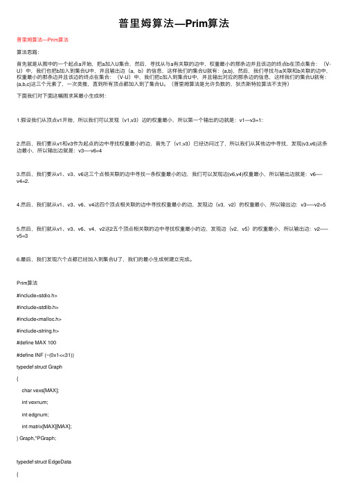
普⾥姆算法—Prim算法普⾥姆算法—Prim算法算法思路:⾸先就是从图中的⼀个起点a开始,把a加⼊U集合,然后,寻找从与a有关联的边中,权重最⼩的那条边并且该边的终点b在顶点集合:(V-U)中,我们也把b加⼊到集合U中,并且输出边(a,b)的信息,这样我们的集合U就有:{a,b},然后,我们寻找与a关联和b关联的边中,权重最⼩的那条边并且该边的终点在集合:(V-U)中,我们把c加⼊到集合U中,并且输出对应的那条边的信息,这样我们的集合U就有:{a,b,c}这三个元素了,⼀次类推,直到所有顶点都加⼊到了集合U。
(普⾥姆算法是允许负数的,狄杰斯特拉算法不⽀持)下⾯我们对下⾯这幅图求其最⼩⽣成树:1.假设我们从顶点v1开始,所以我们可以发现(v1,v3)边的权重最⼩,所以第⼀个输出的边就是:v1—v3=1:2.然后,我们要从v1和v3作为起点的边中寻找权重最⼩的边,⾸先了(v1,v3)已经访问过了,所以我们从其他边中寻找,发现(v3,v6)这条边最⼩,所以输出边就是:v3—-v6=43.然后,我们要从v1、v3、v6这三个点相关联的边中寻找⼀条权重最⼩的边,我们可以发现边(v6,v4)权重最⼩,所以输出边就是:v6—-v4=2.4.然后,我们就从v1、v3、v6、v4这四个顶点相关联的边中寻找权重最⼩的边,发现边(v3,v2)的权重最⼩,所以输出边:v3—–v2=55.然后,我们就从v1、v3、v6、v4,v2这2五个顶点相关联的边中寻找权重最⼩的边,发现边(v2,v5)的权重最⼩,所以输出边:v2—–v5=36.最后,我们发现六个点都已经加⼊到集合U了,我们的最⼩⽣成树建⽴完成。
Prim算法#include<stdio.h>#include<stdlib.h>#include<malloc.h>#include<string.h>#define MAX 100#define INF (~(0x1<<31))typedef struct Graph{char vexs[MAX];int vexnum;int edgnum;int matrix[MAX][MAX];} Graph,*PGraph;typedef struct EdgeData{char start;char end;int weight;} EData;static int get_position(Graph g,char ch){int i;for(i=0; i<g.vexnum; i++)if(g.vexs[i]==ch)return i;return -1;}Graph* create_graph(){char vexs[]= {'A','B','C','D','E','F','G'};int matrix[][7]={{0,12,INF,INF,INF,16,14},{12,0,10,INF,INF,7,INF},{INF,10,0,3,5,6,INF},{INF,INF,3,0,4,INF,INF},{INF,INF,5,4,0,INF,8},{16,7,6,INF,2,0,9},{14,INF,INF,INF,8,9,0}};int vlen=sizeof(vexs)/sizeof(vexs[0]);int i,j;Graph *pG;if((pG=(Graph*)malloc(sizeof(Graph)))==NULL) return NULL;memset(pG,0,sizeof(pG));pG->vexnum=vlen;for(i=0; i<pG->vexnum; i++)pG->vexs[i]=vexs[i];for(i=0; i<pG->vexnum; i++)for(j=0; j<pG->vexnum; j++)pG->matrix[i][j]=matrix[i][j];for(i=0; i<pG->vexnum; i++){for(j=0; j<pG->vexnum; j++){if(i!=j&&pG->matrix[i][j]!=INF)pG->edgnum++;}}pG->edgnum/=2;return pG;}void print_graph(Graph G){int i,j;printf("Matrix Graph: \n");for(i=0; i<G.vexnum; i++){for(j=0; j<G.vexnum; j++)printf("%10d ",G.matrix[i][j]);printf("\n");}}EData* get_edges(Graph G){EData *edges;edges=(EData*)malloc(G.edgnum*sizeof(EData)); int i,j;int index=0;for(i=0; i<G.vexnum; i++){for(j=i+1; j<G.vexnum; j++){if(G.matrix[i][j]!=INF){edges[index].start=G.vexs[i];edges[index].end=G.vexs[j];edges[index].weight=G.matrix[i][j];index++;}}}return edges;}void prim(Graph G,int start){int min,i,j,k,m,n,sum;int index=0;char prim[MAX];int weight[MAX];prim[index++]=G.vexs[start];for(i=0; i<G.vexnum; i++)weight[i]=G.matrix[start][i];weight[start]=0;for(i=0; i<G.vexnum; i++){//i⽤来控制循环的次数,每次加⼊⼀个结点,但是因为start已经加⼊,所以当i为start是跳过 if(start==i)continue;j=0;k=0;min=INF;for(k=0; k<G.vexnum; k++){if(weight[k]&&weight[k]<min){min=weight[k];j=k;}}sum+=min;prim[index++]=G.vexs[j];weight[j]=0;for(k=0; k<G.vexnum; k++){if(weight[k]&&G.matrix[j][k]<weight[k])weight[k]=G.matrix[j][k];}}// 计算最⼩⽣成树的权值sum = 0;for (i = 1; i < index; i++){min = INF;// 获取prims[i]在G中的位置n = get_position(G, prim[i]);// 在vexs[0...i]中,找出到j的权值最⼩的顶点。

应⽤运筹学基础:线性规划(4)-对偶与对偶单纯形法这⼀节课讲解了线性规划的对偶问题及其性质。
引⼊对偶问题考虑⼀个线性规划问题:$$\begin{matrix}\max\limits_x & 4x_1 + 3x_2 \\ \text{s.t.} & 2x_1 + 3x_2 \le 24 \\ & 5x_1 + 2x_2 \le 26 \\ & x \ge0\end{matrix}$$ 我们可以把这个问题看作⼀个⽣产模型:⼀份产品 A 可以获利 4 单位价格,⽣产⼀份需要 2 单位原料 C 和 5 单位原料 D;⼀份产品 B 可以获利 3 单位价格,⽣产⼀份需要 3 单位原料 C 和 2 单位原料 D。
现有 24 单位原料 C,26 单位原料 D,问如何分配⽣产⽅式才能让获利最⼤。
但假如现在我们不⽣产产品,⽽是要把原料都卖掉。
设 1 单位原料 C 的价格为 $y_1$,1 单位原料 D 的价格为 $y_2$,每种原料制定怎样的价格才合理呢?⾸先,原料的价格应该不低于产出的产品价格(不然还不如⾃⼰⽣产...),所以我们有如下限制:$$2y_1 + 5y_2 \ge 4 \\ 3y_1 + 2y_2 \ge3$$ 当然也不能漫天要价(也要保护消费者利益嘛- -),所以我们制定如下⽬标函数:$$\min_y \quad 24y_1 + 26y_2$$ 合起来就是下⾯这个线性规划问题:$$\begin{matrix} \min\limits_y & 24y_1 + 26y_2 \\ \text{s.t.} & 2y_1 + 5y_2 \ge 4 \\ & 3y_1 + 2y_2 \ge 3 \\ & y \ge 0\end{matrix}$$ 这个问题就是原问题的对偶问题。
对偶问题对于⼀个线性规划问题(称为原问题,primal,记为 P) $$\begin{matrix} \max\limits_x & c^Tx \\ \text{s.t.} & Ax \le b \\ & x \ge 0\end{matrix}$$ 我们定义它的对偶问题(dual,记为 D)为 $$\begin{matrix} \min\limits_x & b^Ty \\ \text{s.t.} & A^Ty \ge c \\ & y \ge 0\end{matrix}$$ 这⾥的对偶变量 $y$,可以看作是对原问题的每个限制,都⽤⼀个变量来表⽰。
翻译以下英文术语,并深入了解术语的含义。
1.optimal solution:最优解,使目标函数取得最大值的可行解。
P352.objective function:目标函数,指需优化的量,即欲达的目标,用决策变量的表达式表示。
P123.feasible region:可行域,指所有可行解的集合。
P284. simplex method:单纯形法:是一种迭代的算法,其核心思想是不仅将取值范围限制在顶点上,而且保证每换一个顶点,目标函数值都有所改善.P1175. BF solutions:基可行解,满足变量非负约束条件的基解称为基可行解。
P1816. sensitivity analysis:敏感性分析:指对系统或事物因周围条件变化显示出来的敏感程度的分析。
P1467. algorithm:算法,指系统的求解过程。
p1078. spanning tree:生成树,若有限图的生成子图是一棵树,则称为该图的生成树。
树指不含有圈的连通网。
P3799. states:状态,各阶段开始时的客观条件. P44510.directed arc:有向弧,指通过一条弧的流只有一个方向的弧。
P37611. unbounded:无界,指约束条件不能阻止目标函数值在有利的方向上(正的或者负的)增长。
P3512. CPF solution:顶点(角点)可行解,指位于可行域顶点的解。
P3713. functional constraints:约束条件,指决策变量取值时受到的各种资源条件的限制,通常表达为含决策变量的等式或不等式。
P3414 multiple optimal solutions:多个最优解的问题,指有无穷多解,每一个解都有相同的目标函数值的问题。
P12215. slack variable:松弛变量,添加x i到约束条件的不等式中使其变为等式的变量P10816. augmented solution:增广解,指原始变量(决策变量)取值再加入相应的松弛变量取值后而形成的解。
3. 初始对偶可行基本解的获得⏹刚才所讲的对偶单纯形法是要求有一个初始的对偶可行基本解。
如果我们拿到的是一个不含初始对偶可行基本解,但又要求我们用对偶单纯形法求解时,我们就无能为力了,为此我们还必须研究初始的对偶可行基本解的获得。
⏹这里需要我们构造一个扩充问题,试图通过求解扩充问题而获得初始的对偶可行基本解。
不妨设原问题:1111111221122211110m m k k n n m m k k n n m mm m mk k mn n mm m k k n n x a x a x a x b x a x a x a x b x a x a x a x b c x c x c x z +++++++++++++=+++++=+++++=+++++=−构造的扩充问题为:1111111*********m m k k n nm m k k n nm mm m mk k mn nm x a x a x a x b x a x a x a x b x a x a x a x b +++++++++++=+++++=+++++=max ..0B j j j n mz cx s t x P x bx ∈−=+=≥∑11m k n n x x x x M++++++++= 110m m k k n nc x c x c x z +++++++=− 即:1max ..(*)0,1,,1B j j j n mj n j n mj z cxs t x P x bx x Mx j n ∈−+∈−=+=+=≥=+∑∑其中M 是很大的数。
则系数矩阵前m 列和第n+1列组成的m+1阶单位矩阵可为扩充问题的一个基,立即得到:1,0,B Bj n x b x x j n m x M +′===∈−这个基不一定是对偶可行的。
不失一般性,我们假设是不可行的,但需要说明的是,由此出发可以求得该扩充问题的一个对偶可行基。
即:现在假定让新加入的变量x n+1离基,由于对偶基不可行,必然有判别数大于0,选取最大判别数的非基变量进基,即σk =max {σj |σj >0}则通过旋转运算后的新判别数为:11kj j m jm ka a σσσ++′=−0j j k σσσ′∴=−≤所以旋转运算后所得的新基为对偶可行基。
不连续介质反演的原对偶牛顿法和全变差正则化冯立新;李媛;张磊【摘要】研究利用散射场测量数据反演非均匀介质的逆散射问题,特别是平面波在非均匀介质中传播时所产生逆散射问题的数值计算.为克服非均匀介质不连续变化和反演具有不适定性的困难,提出基于全变差正则化的原对偶牛顿方法,避免了一般正则化方法对不连续介质交界处反演的过光滑性作用.数值试验显示,本算法可以在观测数据带有一定噪声的境况下有效地重构不连续介质系数.%An inverse scattering problem of inhomogeneous mediums from the measurements of the scattered field is considered.In particular,it focuses on the numerical computation of the inverse scattering generated by the interaction of a plane wave and an inhomogeneous medium.To solve the ill-posedness as well as the difficulties caused by inhomogeneous media,a primal-dual Newton method based on the total variation regularization is constructed.The overly smooth effect of the usual regularization method for the inversion is overcome.Numerical experiments show that this method can recover discontinuous coefficients under moderate amount of noise in the observation data.【期刊名称】《黑龙江大学自然科学学报》【年(卷),期】2018(035)001【总页数】9页(P1-9)【关键词】全变差正则化;原对偶牛顿法;逆介质散射【作者】冯立新;李媛;张磊【作者单位】黑龙江大学数学科学学院,哈尔滨150080;黑龙江大学数学科学学院,哈尔滨150080;黑龙江大学数学科学学院,哈尔滨150080【正文语种】中文【中图分类】O1750 IntroductionIn this paper, we focus on the inverse medium scattering problem of determining electromagnetic properties of unknown inhomogeneous objects embedded in a homogeneous background from noisy measurements of the scattered field corresponding to one incident wave impinged on the objects. We describe the scattering model mathematically as follows:Δu(x)+k2η(x)u(x)=0, x∈R2,(1)where u is the total field, k is the wavenumber, η(x)>0 for all x, andm(x)=1-η(x) is the scatterer with a compact support. We assume that B containing the compact support of the scatterer m(x) be a bounded domain in R2. Let ui which is assumed to satisfyΔui+k2ui=0, x∈R2,(2)denote the incident on the inhomogeneity. Assume that the incident fieldui is a plane wave, i.e., ui(x)=exp(ikd·x), where d∈R2 is the propagation direction (a unit vector). The total field u consists of the incident field ui and the scattered field us, that is,u=ui+us.It follows immediately from Eqs. (1) and (2) that the scattered field satisfies Δus+k2us=k2m(x)ui, x∈R2,(3)and the scattered field is required to satisfy the following Sommerfeld radiation condition(4)uniformly in all directions x/|x|.The inverse medium scattering problems arise naturally in many applications such as geophysical exploration, medical imaging, and radar detection [1-5]. For the practical significance of the inverse problem, some inverse scattering methods have been developed in the literature, which may be divided into two categories: the direct methods and the indirect methods. The direct methods aims at detecting the scatterer support and shape, and includes linear sampling method (LSM)[6-8], factorization method (paper [9], Chapter 5, paper [10]), and multiple signal classification (MUSIC)[11-13]. In contrast, the indirect methods provides a distributed estimate of the refractive index by applying regularization techniques. We just mention recursive linearization [14-18] , Gauss-Newton method [19-21], and level set method [22] for an incomplete list. Generally, theestimates by an indirect method can provide more details of inclusions, but at the expense of increased computational efforts. There has been considerable interest in considering efficient and stable inversion techniques. However, due to the strong nonlinearity of the map from the refractive index to the scattered field, severe ill-posedness of the inverse problem and the limited availability of the scattered data, it is still a very challenging problem.In this work, we assume that the scattered data with fixed wavenumber are known in the domain B, i.e., the scattered field is measured forxj∈B,j=1,…,J for a given incident field. We develop an iterated method for accurately detecting the scatterer support. In the case, from the Lippmann-Schwinger integral equation, the inverse problem can be seen as the operator equation of the first kind with unknown m(x). An efficient numerical method is presented for solving the inverse medium scattering problem which is to reconstruct the inhomogeneous medium from inner measurements of the scattered field. We construct the total variation (TV) regularization approximation of the integral equation. The main reason of choosing TV regularization is that TV can penalize highly oscillatory solutions while allowing jumps in the regularized solution. Consequently, a primal-dual Newton method is used to minimize the TV functional [23-25]. This is an iterated method, which need solve direct scattering problem for each step of the process. The scattering data is generated by numerical solution of the direct scattering problem, which is implemented by using the efficient fast algorithm [26]. In this work, we develop a TVregularization and primal-dual method for solving the inverse medium problem with discontinuous coefficients. The remainder of the paper is organized as follows. Section 1 gives the integral formulation of inverse medium problem (1)~(4) and describes the TV regularization approximation. In Section 2, we employ a primal-dual Newton method for solving the corresponding inverse problem. Section 3 presents the numerical results for the inverse medium problem. Finally, we give the relevant conclusions in Section 4.1 Formulation of the integral equation and TV approximationThe integral formulation of problem (1)~(4) is the main ingredient in the proposed method. Let be the Hankel function of first kind and order 0, see paper [1] for details. We have the following Lippmann-Schwinger integral equation for u:(5)K(x,y)m(y)dy.So, we have following operator equation(Km)(x)=g.Define the Tikhonov-TV functional(6)where TV(m) is the TV of a function m defined on the B. If m is smooth, one can obtain the representation|m|dx.However, the representation is not suitable for the implementation of the numerical procedure, due to the nondifferentiability of the Euclidean norm at the origin. To overcome this difficulty, one can take an approximation to the Euclidean norm |x| like where β is a small positive parameter. This yields the following approximation to TV(m):Instead of the Tikhonov-TV functional (6), we will consider minimization of the functional(7)Suppose m=mi,j is defined on an equispaced grid in two space dimensions, {(x1i,x2j)|x1i=iΔx1,x2j=jΔx2,i=0,…,n1,j=0,…,n2}. We defi ne the discrete penalty functional Jβ(m):R(n1+1)×(n2+1)→R by(8)where To simplify notation, we drop a factor of Δx1Δx2 from the right-hand side of (8). This factor can be absorbed in the regularization α in (7). In the following section, we consider minimization of the discretized functional:(9)where the matrix K is a discretization of the operator K, the vector g and J denote discrete data, and discretization of TV approximation Jβ,respectively.2 A primal-dual Newton methodTo minimize the functional (9), the primal-dual Newton method is employed. Consider the convex functional defined on C=R2. One can show that the conjugate set C* is the unit ball in R2 and corresponding conjugate functional to φβ is(10)We can obtain the dual representation by (10):(11)The following theorem relates the gradient of a convex functional φβ to the gradient of its conjugate see paper [25], p.138 for a proof.Theorem 1 Suppose that φβ is differentiable in a neighborhood ofx0∈C⊂Rd, and the mapping F=gradφβ:Rd→R d is invertible in that neighborhood. Then is Frechét differentiable in a neighborhood ofy0=φβ(x0) withEmploying the dual representation (11), we obtain(12)We stack the array components mi,j,ui,j and vi,j into column vector m,u, and v, let Dx1 and Dx2 be matrix representation for the grid operators and and let <·,·> denote the Euclidean inner product. Then (12) can be rewritten asMinimization of the least squares functional (10) is equivalent to computing the saddle point(u*,v*,m*(13)where We refer to m as the primal variable, and to u and v as the dual variables.Since (13) is unconstrained with respect to m, a first order necessary condition for a saddle point is(14)An additional necessary condition is that the duality gap in (11) must vanish, i.e., for each grid index i, j,(15)Finally, the dual variables must lie in the conjugate set, i.e.,(ui,j,vi,j)∈C*.(16)Suppose (15) holds for a point (ui,j,vi,j) in the interior of C*. ThenUsing Theorem 1, above equations is equivalent toDx1m=B(m)u, Dx2m=B(m)v,(17)where B(m)=diag(1/ψ′(m)).We can reformulate the first order necessary conditions (14) and (17) as a nonlinear system:(18)The derivative of G can be expressed asHere B′(m)u has matrix representationB′(m)u-Dx1=-E11Dx1-E12Dx2(19)withwhere the products and quotients are computed pointwise. Similarly,B′(m)v-Dx2=-E21Dx1-E22Dx2(20)withNewton’s method for the system (18) requires solutions of systems of the formG′(u,v,m)(Δu,Δv,Δm)=-G(u,v,m).Substituting (19)~(20) and app lying block row reduction to convert G′ to block upper triangular form, consequently we obtainwhereandWe employ backtracking to the boundary to maintain the constraint (16). In other words, we computeall i,j}.We then updateAlgorithm Primal-dual Newton’s method for TV functional.ν:=0;m0:=initial guess for primal variable;u0,v0:=initial guess for dual variables;begin primal-dual Newton iterations;Δm:=[KTK+αLν]-1rν;mν+1:=mν+Δm;τν:=max{0≤τ≤1|(uν+τΔu,vν+τΔv)∈C*};uν+1:=uν+τνΔu;vν+1:=vν+τνΔv;ν:=ν+1;end primal-dual Newton iteration.3 Numerical experimentsSome numerical examples are presented to illustrate the performance of the proposed method. Here, the scattering data are generated by numerical solution of the direct scattering problem, which is implemented by using the efficient fast algorithm (see Appendix).In experiments we consider the following inhomogeneities,★ the scattered fields are measured on the domain B=[-2,2]×[-2,2];★ the incident direction d=(cos(π/3),sin(π/3)), and wa ve number k=1;★ {Qi,j⊂R2,i=1,2,…,n1,j=1,2,…,n2} is a partition of B;★ the parameters n1=20(40),n2=20(40), α=0.001, β=0.05.Fig.1 True scatterer (n1)Fig.2 Reconstruction n1 using primal-dual Newton’s methodFig.3 True scatterer (n2)Fig.4 Reconstruction n2 using primal-dual Newton’s methodTo test the stability, some relative random noise is added to the data, i.e., the measurement data takes the formu|B:=(1+δrand)u|B,where ‘rand’ gives the Gaussian white noise and δ is a noise level parameter taken to be 5% in our numerical experiments.We have set the parameter α in the TV formulation. Then, we use the above primal-dual Newton’s algorithm to solve the inverse problem. The stopping criterion for the iteration is a relative decrease of the nonlinear residual by a factor of 10-4 or through 50 times iterations. Here, the initial guess for m can be chosen for different constant. The reconstruction got faster when the the initial guess for m is better. Fig.2 and Fig.4 present reconstruction results of the refractive index from the measurement data. We can see that the method has the ability to resolve the inverse medium problem with discontinuous coefficients efficiently.4 ConclusionsWe have proposed and discussed a reconstruction technique of the inverse medium problem with discontinuous coefficients based on the measurements of the scattering field. Our aim to overcome the difficulties caused by the the ill-posedness as well as the difficulties caused by inhomogeneous media has been realized. To make the discontinuous coefficients of the medium can be reliably reconstructed, we convert the problem to an equivalent optimization problem, and then introduce the regularization term. At the same time, we use primal dual Newton method to solve the above problem. Finally, an inversion algorithm, based on TV regularization, for the inverse medium problem from the measurement data of the scattered field is shown. Numerical experiments show that the method is effective.AppendixHere, we give a fast algorithm to solve forward scattering problem (1)~(4).The method was proposed by Nadaniela Egidi etc, see paper [26] for details. The problem (1)~(4) can be reformulated as a Fredholm integral equation (5) of the second kind:Let {Ql,j⊂R2,l=1,2,…,n1,j=1,2,…,n2} be a p artition of B, the integral equation (5) is discretized as follows:(21)where ξl,j∈R2 is the center of ml,j=m(ξl,j), and ul,j is an approximation of u(ξl,j). Linear system (21) can be rewritten as following formAu=b,where b∈Cn1n2 contains u∈Cn1n2 contains ul, j, and the entry of matrix A, at row corresponding to indices l,j, and at column corresponding to i1, j1, containswhere δ is the Kronecker function.In following we give an approximation of the coefficient matrix A by using the properties of Hankel functions We havewhere J0 is the Bessel function of order 0, and Y0 is the Newmann function of order 0. From the power series expansions of these functions we have tlρ2l, ρ>0,where γ≈0.577 215 7 is the Euler constant, andhere B>0 is a suitable constant that depends on the size of D, and L is a truncation parameter.Substituting above express into (21), we obtain the following linear system:(22)where is the approximation of ul,j .We restrict our attention to coordinate partitions of B, whereQl,j,l=1,…,n1,j=1,…,n2 are given by rectangles having edges parallel to the coordinate axes. Moreover, we use the following notations :Ql,j=[al,bl]×[aj,bj],ξl,j=(ξ1l,ξ2j)∈R2,l=1,…,n1,j=1,…,n2. So, calculating the integral in (22), and rearranging the resulting terms, we obtain-×(-ξ1l)2q+1-l(-ξ2j)2p-2q+1-s)-,l=1,…,n1,j=1,…,n2.(23)Linear system (23) can be solved efficiently due to the special structure of its coefficient matrix, which is given by the identity matrix plus 2(L+1)2 rank-one matrices. We conclude that (23) can be rewritten as follows :(I+UVT)u=b,where U,V are following complex matrices having n1n2 rows and 2(L+1)2 columns.here×(-ξ1,i1)2q+1-l(-ξ2,i2)2p-2q+1-s,i1=1,2,...,n1,i2=1,2,...,n2,M=2L+1,N(l)=2L-2⎣l/2」+1.References[1] COLTON D, KRESS R. Inverse acoustic and electromagnetic scattering theory [M]. Berlin: Springer-Verlag, 1998.[2] CUI T J, CHEW W C, AYDINER A. Inverse scattering of two-dimensional dielectric objects buried in a lossy earth using the distorted Born iterative method [J]. IEEE Transactions on Geoscience and Remote Sensing, 2001, 39(2): 339-346.[3] BAO G, LI P. Numerical solution of an inverse medium scattering problem for Maxwell’s equations at fixed frequency [J]. Journal of Computational Physics, 2009, 228(12): 4638-4648.[4] BAO G, CHOW S N, LI P, et al. Numerical solution of an inverse medium scattering problem with a stochastic source [J]. Inverse Problems, 2010, 26 (7): 74014.[5] BAO G, LIN J, MEFIRE S M. Numerical reconstruction of electromagnetic inclusions in three dimensions [J]. SIAM Journal on Imaging Sciences, 2014, 7(1): 558-577.[6] CAKONI F, COLTON D, MONK P. The linear sampling method in inverse electromagnetic scattering [M]. Philadelphia: SIAM, 2010.[7] ITO K, JIN B, ZOU J. A direct sampling method to an inverse medium scattering problem [J]. Inverse Problems, 2012, 28(2): 25003.[8] ITO K, JIN B, ZOU J. A direct sampling method for inverse electromagnetic medium scattering [J]. Inverse Problems, 2013, 29(9): 95018.[9] KIRSCH A, GRINBERG N. The factorization method for inverse problems [M]. Oxford: Oxford University Press, 2008.[10] KIRSCH A. The MUSIC-algorithm and the factorization method in inverse scattering theory for inhomogeneous media [J]. Inverse Problems, 2002, 18(4): 1025-1040.[11] AMMARI H, IAKOVLEVA E, LESSELIER D, et al. MUSIC-type electromagnetic imaging of a collection of small three-dimensional inclusions [J]. SIAM Journal on Scientific Computing, 2007, 29(2): 674-709.[12] CHEN X D, ZHONG Y. MUSIC electromagnetic imaging with enhanced resolution for small inclusions [J]. Inverse Problems, 2009, 25(1): 15008. [13] BAO G, HOU S, LI P. Inverse scattering by a continuation method with initial guesses from a direct imaging algorithm [J]. Journal of Computational Physics, 2007, 227(1): 755-762.[14] BAO G, LI P. Inverse medium scattering for the Helmholtz equation at fixed frequency [J]. Inverse Problems, 2005, 21(5): 1621-1641.[15] BAO G, LI P. Numerical solution of inverse scattering for near-field optics [J]. Optics Letters, 2007, 32(11): 1465-1467.[16] BAO G, LIU J. Numerical solution of inverse scattering problems with multi-experimental limited aperture data [J]. SIAM Journal on ScientificComputing, 2003, 25(3): 1102-1117.[17] BAO G, TRIKI F. Error estimates for the recursive linearization of inverse medium problems [J]. Journal of Computational Mathematics, 2010, 28(6): 725-744.[18] BAO G, LI P, LIN J, et al. Inverse scattering problems with multi-frequencies [J]. Inverse Problems, 2015, 31 (9): 93001.[19] ZAEYTIJD D J, FRANCHOIS A, EYRAUD C, et al. Full-wave three-dimensional microwave imaging with a regularized Gauss-Newton method-theory and experiment [J]. IEEE Transactions on Antennas and Propagation, 2007, 55(11): 3279-3292.[20] HOHAGE T, LANGER S. Acceleration techniques for regularized Newton methods applied to electromagnetic inverse medium scattering problems [J]. Inverse Problems, 2010, 26(7): 74011.[21] KRESS R, RUNDELL W. Inverse scattering for shape and impedance [J]. Inverse Problems, 2001, 17(4): 1075-1085.[22] DORN O, LESSELIER D. Level set methods for inverse scattering: some recent developments [J]. Inverse Problems, 2009, 25(12): 125001.[23] BAO G, HUANG K, LI P, et al. A direct imaging method for inverse scattering using the generalized Foldy-Lax formulation [J]. Contemporary Mathematics, 2014, 615: 49-70.[24] CHAN T F, GOLUB G H, MULET P. A nonlinear primal-dual method for total varlation-based 冯立新image restoration [J]. SIAM Journal on Scientific Computing, 1999, 20(6): 1964-1977.[25] VOGEL C R. Computational methods for inverse problems [J].Philadelphia: SIAM, 2002.[26] EGIDI N, GOBBI R, MAPONI P. The efficient solution of electromagnetic scattering for inhomogeneous media [J]. Journal of Computational and Applied Mathematics, 2007, 210(1-2): 175-182.。
集合覆盖问题的模型与算法王继强【摘要】The set cover problem has favourable applications in areas of network design, but it is NP-hard in computational com-plexity. A 0-1 program model is formulated for the set cover problem. An approximation algorithm deriving from greedy idea is put forward, and is proved from the angle of primal-dual program. A case study of sensor network optimal design based on LINGO software demonstrates correctness of the model and effectiveness of the algorithm.% 集合覆盖问题在网络设计领域中有着良好的应用背景,但它在算法复杂性上却是NP-困难问题。
建立了集合覆盖问题的0-1规划模型,给出了源于贪心思想的近似算法,并从原始-对偶规划的角度进行了证明,基于LINGO软件的传感器网络最优设计案例验证了模型的正确性和算法的有效性。
【期刊名称】《计算机工程与应用》【年(卷),期】2013(000)017【总页数】4页(P15-17,72)【关键词】集合覆盖;近似算法;0-1规划;对偶规划;线性交互式通用优化器(LINGO)【作者】王继强【作者单位】山东财经大学数学与数量经济学院,济南 250014【正文语种】中文【中图分类】Q784;TP301.61 引言集合覆盖问题是组合最优化和理论计算机科学中的一类典型问题,它要求以最小代价将某一集合利用其若干子集加以覆盖。