基于HyperWorks的某通风盘式制动器热-结构分析

课程设计任务书目录1、实体建模步骤、、、、、、、、、、、、、、、、、、、、、、、、、、、、、、、、、、、、、、、、、、、、、、、、、、、、、、、31、1制动盘建模、、、、、、、、、、、、、、、、、、、、、、、、、、、、、、、、、、、、、、、、、、、、、、、、、、、、31、2摩擦片建模、、、、、、、、、、、、、、、、、、、、、、、、、、、、、、、、、、、、、、、、、、、、、、、、、、、、41、3制动活塞建模、、、、、、、、、、、、、、、、、、、、、、、、、、、、、、、、、、、、、、、、、、、、、、、、、、61、4制动钳建模、、、、、、、、、、、、、、、、、、、、、、、、、、、、、、、、、、、、、、、、、、、、、、、、、、、、61、5整体装配、、、、、、、、、、、、、、、、、、、、、、、、、、、、、、、、、、、、、、、、、、、、、、、、、、、、、、82、导入过程、、、、、、、、、、、、、、、、、、、、、、、、、、、、、、、、、、、、、、、、、、、、、、、、、、、、、、、、、、、93、有限元分析得过程分析得过程、、、、、、、、、、、、、、、、、、、、、、、、、、、、、、、、、、、、、、、、103、1对导入得模型进行单元属性定义、、、、、、、、、、、、、、、、、、、、、、、、、、、、、、、、、103、2网格划分及添加约束、、、、、、、、、、、、、、、、、、、、、、、、、、、、、、、、、、、、、、、、、、、103、3进行模态分析、、、、、、、、、、、、、、、、、、、、、、、、、、、、、、、、、、、、、、、、、、、、、、、、、113、4制动盘得振型分析、、、、、、、、、、、、、、、、、、、、、、、、、、、、、、、、、、、、、、、、、、、、、123、5结论、、、、、、、、、、、、、、、、、、、、、、、、、、、、、、、、、、、、、、、、、、、、、、、、、、、、、、、、、15参考文件、、、、、、、、、、、、、、、、、、、、、、、、、、、、、、、、、、、、、、、、、、、、、、、、、、、、、、、、、、、、161 实体建模步骤建模选用catia三维操作软件,建模步骤如下。

通风式制动盘热性能理论与有限元仿真分析研究汪元健;陈先兵【摘要】从解决整车抖动实际问题出发,以制动盘热性能影响抖动为切入点,详细介绍了热性能分析的理论基础,并通过建立制动盘热-固耦合有限元模型,利用有限元分析软件进行热性能仿真分析,并用专业台架模拟实车制动进行相关的实验,将试验数值与仿真数值进行比较,验证有限元分析结果的可靠性与准确性,从而得到更优的制动盘结构.【期刊名称】《汽车零部件》【年(卷),期】2018(000)009【总页数】5页(P57-61)【关键词】通风制动盘;热性能;热-固耦合模型;有限元分析【作者】汪元健;陈先兵【作者单位】浙江力邦合信智能制动系统股份有限公司,浙江温州325400;浙江力邦合信智能制动系统股份有限公司,浙江温州325400【正文语种】中文【中图分类】U461.30 引言随着中国汽车工业的快速发展、国内汽车保有量的迅猛增加以及人们生活水平的不断提高，汽车的安全性与舒适性也随之受到人们越来越多的关注，其中汽车制动系统的可靠性与车辆的安全性、舒适性息息相关，而制动系统中制动盘的热性能表现又在汽车制动系统中扮演着一个关键的角色。

制动盘的热性能指的是汽车在制动时，制动盘与摩擦片之间由于摩擦产生大量的热量，其中大部分的热量分散在制动盘内，大量的热会使制动盘的温度急剧升高，引起制动盘的热膨胀和热变形，导致制动盘表面产生热点，进而增加制动盘的端面跳动值，引发制动时盘和片之间制动力和制动力矩的波动，从而引起整个制动器的抖动。

抖动的发生除了会降低乘车舒适性，还会加剧车辆相关零部件的磨损，即加快疲劳破坏，进而影响车辆本身的安全性。

因此改善制动器制动盘的热性能表现对于整车的安全性与舒适性尤为重要。

以某公司研发的一款制动器为例，详细介绍了通风式制动盘热性能分析的理论基础，通过建立热-固耦合分析模型，在多次连续循环制动工况下研究制动盘的温度与热变形情况，通过仿真数值与实验数据对比分析验证制动盘热-固耦合模型的合理性与准确性。

图解汽车（12）汽车制动系统结构解析● 制动系统的组成作为制动系统，作用当然就是让行驶中的汽车按我们的意愿进行减速甚至停车。

工作原理就是将汽车的动能通过摩擦转换成热能。

汽车制动系统主要由供能装置、控制装置、传动装置和制动器等部分组成，常见的制动器主要有鼓式制动器和盘式制动器。

● 鼓式制动器鼓式制动器主要包括制动轮缸、制动蹄、制动鼓、摩擦片、回位弹簧等部分。

主要是通过液压装置是摩擦片与岁车轮转动的制动鼓内侧面发生摩擦，从而起到制动的效果。

在踩下刹车踏板时，推动刹车总泵的活塞运动，进而在油路中产生压力，制动液将压力传递到车轮的制动分泵推动活塞，活塞推动制动蹄向外运动，进而使得摩擦片与刹车鼓发生摩擦，从而产生制动力。

从结构中可以看出，鼓式制动器是工作在一个相对封闭的环境，制动过程中产生的热量不易散出，频繁制动影响制动效果。

不过鼓式制动器可提供很高的制动力，广泛应用于重型车上。

●盘式制动器盘式制动器也叫碟式制动器，主要由制动盘、制动钳、摩擦片、分泵、油管等部分构成。

盘式制动器通过液压系统把压力施加到制动钳上，使制动摩擦片与随车轮转动的制动盘发生摩擦，从而达到制动的目的。

与封闭式的鼓式制动器不同的是，盘式制动器是敞开式的。

制动过程中产生的热量可以很快散去，拥有很好的制动效能，现在已广泛应用于轿车上。

● 通风制动盘制动过程实际上是摩擦力将动能转化为热能的过程，如制动器的热量不能及时散出，将会影响其制动效果。

为了进一步提升制动效能，通风制动盘应运而生。

通风刹车盘内部是中空的或在制动盘打很多小孔，冷空气可以从中间穿过进行降温。

从外表看，它在圆周上有许多通向圆心的洞空，它利用汽车在行驶当中产生的离心力能使空气对流，达到散热的目的，因此比普通实心盘式散热效果要好许多。

●陶瓷制动盘陶瓷制动盘相对于一般的刹车盘具有重量轻、耐高温耐磨等特性。

普通的刹车盘在全力制动下容易高热而产生热衰退，制动性能会大打折扣，而陶瓷刹车盘有很好的抗热衰退性能，其耐热性能要比普通制动盘高出许多倍。

基于hyperworks的结构静力学分析实例教程Linear Static Analysis of a Plate with a Hole - RD-1000This tutorial demonstrates how to create finite elements on a given CAD geometry of a plate with a hole, apply boundary conditions, and perform a finite element analysis of the problem. Post-processing tools will be used in HyperView to determine deformation and stress characteristics of the loaded plate.The following exercises are included:Setting up the problem in HyperMeshApplying Loads and Boundary ConditionsSubmitting the jobViewing the resultsExerciseStep 1: Launch HyperMesh and set the RADIOSS (Bulk Data) User Profile/doc/a49962095.htmlunch HyperMesh.A User Profiles… Grap hic User Interface (GUI) will appear. If it does not appear, go to Preferences>User Profiles … from the menu on the top.2.Select RADIOSS in the User Profile dialog.3.From the extended list, select Bulk Data.4.Click OK.This loads the User Profile. It includes the appropriate template, macro menu, and import reader, paring down the functionality of HyperMesh to what is relevant for generating models in Bulk Data Format for RADIOSS and OptiStruct.Step 2: Open the File plate_hole.hm1.Click the Open .hm file icon .An Open file… browser window pops up.2.Select the plate_hole.hm file, located in the HyperWorks installation directory under/tutorials/hwsolvers/radioss/.3.Click Open.The plate_hole.hm database is loaded into the current HyperMesh session, replacing any existing data. The database only contains geometric data.Setting Up the Problem in HyperMeshWhen building models, we encourage you to create the material and property collectors before creating the component collectors. This is the most efficient way of setting up the file since components need to reference materials and properties.Step 3: Create the material1.Click the Material Collector Panel toolbar button .2.Make sure the create subpanel is selected using the radio buttons on the left-hand side of the panel.3.Click mat name = and enter steel.4.Select the desired color for the material steel by clicking on .5.Click type = and select ISOTROPIC.6.Click card image = and select MAT1.7.Click create/edit.The MAT1 card image pops up.If a material property in brackets does not have a value below it, it is off. To edit these materialproperties, click the property in brackets you wish to edit and an entry field will appear below it. Click the entry field and entera value.8.Enter the following values for E, NU and RHO; E as 2e5; NUas 0.3 and RHO as 7.9e-09.9.Click return twice.A new material, steel, has been created. The material uses RADIOSS's linear isotropic material model,MAT1. This material has a Young's Modulus of 2E+05 and a Poisson's Ratio of 0.3. It is not necessary to define a density value since only a static analysis will be performed. Density values are required,however, for other solution sequences.At any time, the card image for this collector can be modified using the Card Editor .Step 4: Create the properties and update the Component Collector1.Click Properties toolbar icon .2.Make sure the create subpanel is selected using the radio buttons on the left-hand side of the panel.3.Click prop name = and enter plate_hole.4.Select the desired color for the property plate_hole by clicking on .5.Click type = and select 2D.6.Click card image = and select PSHELL.7.Click material = and select steel.8.Click create/edit.The PSHELL card image pops up.9.Click [T] and enter 10.0 as the thickness of the plate.10.Click return twice and go back to the main menu.The property of the shell structure has been created as 2D PSHELL. Material information is also linked to this property.11.Click the Component Collector Panel toolbar button .12.Make sure the update subpanel is selected using the radiobuttons on the left-hand side of the panel.13.Click comps >> and select plate_hole from the list.14.Toggle to property =.15.Click property = twice and select the plate_hole property from the list.Property card image and material information are listed below the property entry field.16.Click update.17.Click return to go to the main menu.The component plate_hole has been updated with a property of the same name and is currently the“Current Component” (see the box in the lower right for plate_hole ). This component uses theplate_hole property definition with a thickness value of 10.0. The material steel is referenced by this component.At any time, the card image for this collector can be modified using the Card Editor and the material referenced by this component collector can be changed using the update option in the Collectors panel.Apply loads and boundary conditions to the modelIn the following steps, the model is constrained so that two opposing edges of the four external edges cannot move. The other two edges remain unconstrained. A total load of 1000N is applied at the edge of the hole in the positive z-direction.Step 5: Create load collectors (spcs and forces )A new load collector, spcs is created.A new load collector, forces is created.Step 6: Create constraints1.Click the Load Collectors toolbar icon .2.Make sure the create subpanel is selected using the radio buttons on the left-hand side of the panel.3.Click loadcol name = and enter spcs .4.Click color and select a color from the color palette.5.Click the creation method switch and select no card image from the pop-up menu.6.Click create .7.Click loadcol name = and enter forces .8.Click color and select a different color from the color palette.9.Click create .10.Click return to go to the main menu.1.From Model Browser expand LoadCollectors , right-click on spcs and click Make current to set spcsas the current load collector.The window is polygonal, and every mouse click creates a window vertex.Illustration of which nodes to select for applying single point constraints. Dofs with a check will be constrained while dofs without a check will be free.Dofs 1, 2, and 3 are x, y, and z translation degrees of freedom.Dofs 4, 5, and 6 are x, y, and z rotational degrees of freedom.This applies these constraints to the selected nodes.Step 7: Create forces on the nodes around the holeThe window is polygonal, and every mouse click creates a window vertex.2.From the Analysis page,enter the constraints panel.3.Make sure the create subpanel is selected using the radiobuttons on the left-hand side of the panel.4.Make sure nodes are selected from the entity selection switch.5.Click nodes and select by window from the pop-up extended entity selection menu.6.Draw a window in the graphics area encompassing the nodes to be selected (shown in the figure).7.Check the box beside interior and click on select entities .8.Constrain dof1, dof2, dof3, dof4, dof5, and dof6 and set all of them to a value of 0.0.9.Ensure the load types is set to SPC .10.Click create .11.Click return to go to the main menu.1.Set your current load collector to forces in Model Browser as shown before in point 1 under Step 6.2.From the Analysis page, enter the forces panel.3.Make sure the create subpanel is selected using the radio buttons on the left-hand side of the panel.4.Make sure nodes are selected from the entity selection switch.5.Click nodes and select by window from the pop-up extended entity selection menu.6.Draw a window in the graphics window encompassing the nodes shown in the figure below.Nodes selected for creating loading around hole.7.Check the box beside interior and click on select entities.8.Set the coordinate system toggle to global system.9.Click the vector definition switch and select constant vector.10.Click magnitude = and enter 21.277 (i.e. 1000 divided by the number of nodes 47).11.Click the direction definition switch below magnitude=, and select z-axis from the pop-up menu.12.Ensure the load types is set to FORCE.13.Click create.This creates a number of point forces, with the given magnitude in the z-direction, to be applied to the nodes about the hole.14.Click return to go to the main menu.Step 8: Create a RADIOSS subcase (also referred to as a loadstep)1.From the Analysis page, enter the loadsteps panel.2.Click name = and enter lateral force.3.Click the type: switch and select linear static, if it is not already selected by default.4.Check the box preceding SPC.An entry field appears to the right of SPC.5.Click on the entry field and select spcs from the list of load collectors.6.Check the box preceding LOAD.An entry field appears to the right of LOAD.7.Click on the entry field and select forces from the list of load collectors.8.Click create.A RADIOSS subcase has been created which references the constraints in the load collector spcs andthe forces in the load collector forces.9.Click return to go to the main menu.Step 9: Submitting the job1.From the Analysis page, enter the RADIOSS panel.2.Click save as… following the input file: field.A Save file… browser window pops up.3.Select the directory where you would like to write the RADIOSS model file and enter the name for themodel, plate_hole.fem, in the File name: field.The .fem filename extension is the recommended extension for RADIOSS Bulk Data Format input decks.4.Click Save.Note the name and location of the plate_hole.fem file displays in the input file: field.5.Set the export options:toggle to all.6.Click the run options: switch and select analysis.7.Set the memory options: toggle to memory default.8.Click Radioss.This launches the RADIOSS job. If the job is successful, you should see new results files in the directory from which plate_hole.fem was selected. The plate_hole.out file is a good place to look for error messages that could help debug the input deck if any errors are present.The default files written to the directory are:plate_hole.html HTML report of the analysis, giving a summary of the problemformulation and the analysis results.plate_hole.out RADIOSS output file containing specific information on the file setup,the setup of your optimization problem, estimates for the amount ofRAM and disk space required for the run, information for eachoptimization iteration, and compute time information. Review this filefor warnings and errors.plate_hole.h3d HyperView binary results file.plate_hole.res HyperMesh binary results file.plate_hole.stat Summary of analysis process, providing CPU information for eachstep during analysis process.Viewing the ResultsDisplacement and Stress results for linear static analyses are output from RADIOSS by default. The following steps describe how to view those results in HyperView.HyperView is a complete post-processing and visualization environment for finite element analysis (FEA), multi-body system simulation, video and engineering data.Step 10: View a contour plot of stresses1.Once you receive the message 'Process Completed Successfully' in the command window, clickHyperView.HyperView is launched and the results are loaded. A message window appears to inform of thesuccessful model and result files loading into HyperView.2.Click Close to close the message window.3.Click the Contour toolbar button .4.Select the first pull-down menu below Result type:and select Element Stresses [2D & 3D] (t).5.Select the second pull-down menu below Result type:and select vonMises.6.Select None in the field below Averaging method:.7.Click Apply.A contoured image representing von Mises stresses should be visible. Each element in the model isassigned a legend color, indicating the von Mises stress value for that element, resulting from the applied loads and boundary conditions.8.Click Top in the view controls from the bottom right corner to view the model, as shown in the followingfigure.von Mises stress assigned plotWhat is the maximum von Mises stress value?At what location does the model have its maximum stress?Does this make sense based on the boundary conditions applied to the model?Step 11: View a contour plot of displacements1.Select the first pull-down menu below Result type:and select Displacement (v).2.Select the second pull-down menu below Result type:and select Mag.3.Click Apply.The resulting contours represent the displacement field resulting from the applied loads and boundary conditions.What is the maximum Displacement value?At what location does the model have its maximum displacement?Does this make sense based on the boundary conditions applied to the model?Step 12: View the deformed shape1.Click Iso in the view controls (bottom right corner) to display the isometric view of the model.2.Click the Deformed toolbar button .3.Set Result type: to Displacement(v), Scale:to Scale factor; and Type:to Uniform.4.In the field next to value, enter 500.This means that the displacement results of the analysis will be multiplied by 500.5.For Show:, select Wireframe.6.Click Apply.A deformed plot of your model with displacement contour should be visible, overlaid on the originalundeformed mesh. Refer to the following figure to see what the plot should look like in isometric view.Isometric view of deformed plot overlaid on the original undeformed mesh with model units set to 500.Go ToRADIOSS, MotionSolve, and OptiStruct Tutorials。

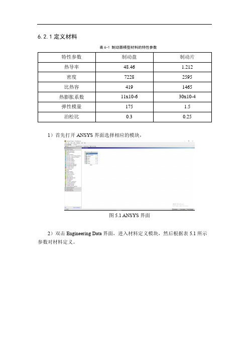
6.2.1定义材料表6-1 制动器模型材料的特性参数1）首先打开ANSYS界面选择相应的模块，图5.1 ANSYS界面2）双击Engineering Data界面，进入材料定义模块，然后根据表5.1所示参数对材料定义。

图5.2 ANSYS材料定义界面6.1.3模型处理将CATIA建立的制动盘模型转成stp格式，再将其导进ANSYS内，创建截面特性和分配截面特性，开展模型的前期处理，处理结果如图5.3所示。

图5.3 模型处理界面6.1.4制动盘的模态分析1）打开ANSYS界面，选择Modal 模块，根据上文对制动盘进行前处理。

图5.4 模态分析界面2）网格划分网格划分结果如下图5.5所示。

图5.5 制动盘网格划分结果3）边界条件设置选择Analysis Settings把Max Modes to Find 数值修改为6 ，选择制动盘的五个螺栓孔，用Fixed Support进行固定约束。

再在Solution添加六个Total Deformation，并把每个Total Deformation调成相应模态阶数的位移。

具体操作如下图所示。

图5.6 约束条件设置图5.7 求解设置4）后处理点击运算按钮，得到的前六阶模态如下图5.8-5.13所示。

图5.8 一阶模态图5.9 二阶模态图5.10 三阶模态图5.11 四阶模态图5.12 五阶模态图5.13 六阶模态图5.8-5.13是制动盘的1-6阶模态振型图。

相关结果可得：第一阶的固有频率为1356.7Hz，振型表现出对称型排列，于其边缘处产生了2处较大应变。

第二阶的固有频率为1380.8Hz，振型结果与第一阶相近。

第三阶的固有频率为1524.9Hz，振型为伞形振型，应变均匀分布在制动盘的边缘。

第四阶的固有频率为1599.1Hz，振型为垂直弯曲振型，在制动盘周边相距60度的地方有6处较大的应变。

第五阶的固有频率为1603.4Hz，该阶振型与第四阶相近。

第六阶的固有频率为2224.2Hz，振型为扭转振型。

基于ABAQUS的刹车盘热应力分析随着机动车数量的不断增加，刹车系统的安全性和使用寿命成为一个重要的研究方向。

刹车盘作为刹车系统的关键部件之一，其材料选择对于提高机动车的安全性能至关重要。

在刹车过程中，由于制动器片和刹车盘之间的不断摩擦，会产生大量的热量并引起刹车盘的热应力，影响刹车盘的性能与使用寿命。

为深入研究刹车盘的热应力，本文采用ABAQUS软件对刹车盘进行热应力分析。

首先，我们需要进行前期工作。

根据实际情况，选取合适的刹车盘模型和材料模型，并设置刹车盘的几何尺寸和初始温度以及制动器片的作用力。

在模型的加工过程中，需要注意刹车盘各部位的加工精度，以保证模型的准确性。

然后，我们对刹车盘进行热传递分析。

刹车盘在刹车过程中会受到大量的制动器片摩擦产生的热量的影响，因此需要对其热传递进行分析。

在计算过程中，我们需要根据实际数据设置以下参数：热扩散系数、材料密度和比热、传热系数等。

这些参数可以在材料手册中获得。

接下来，我们进行热弹性分析。

在高温和大应力的环境下，刹车盘内部会产生热应力，导致刹车盘的力学性能发生变化。

利用ABAQUS软件对于刹车盘的热应力进行分析，可以了解到刹车盘在制动过程中是否发生变形、开裂等破坏现象，预测刹车盘寿命并进行优化设计。

最后，我们将分析结果进行打印和分析，根据热应力分析结果，对刹车盘的合理性进行评估。

如果出现问题，可以尝试通过改变制动片的材料、设置通风方式等方式来解决问题，提高刹车盘的寿命和安全性能。

总的来说，ABAQUS软件提供了一个重要的工具，用于对于刹车盘的热应力进行分析、寿命预测和性能优化。

通过对于刹车盘的热应力分析，我们可以有效提高机动车的安全性和使用寿命，保障行车安全。

刹车盘的热应力分析需要大量的相关数据，从材料的热物理参数到刹车盘的几何尺寸等方面都需要考虑。

下面列举了一些相关数据，并进行分析。

1. 刹车盘材料的热物理参数：例如，材料的热扩散系数、比热和密度等，这些参数会影响刹车盘在制动过程中的热传递和热应力。

10.16638/ki.1671-7988.2020.13.012基于Hyperworks的散热器支架有限元分析及改进设计龙俊华，安瑞兵（广州汽车集团股份有限公司汽车工程研究院，广东广州510000）摘要：文章通过Hyperworks软件对散热器支架进行了仿真分析，判断了散热器支架高强耐久试验时的破坏原因。

对散热器支架方案进行了设计改善，通过改进方案的仿真设计，找出了满足强度要求的方案，为今后的汽车散热器支架设计开发提供了可借鉴的方法。

关键词：散热器支架；有限元分析中图分类号：U462.1 文献标识码：A 文章编号：1671-7988(2020)13-39-03Finite Element Analysis And Improved Design Of Radiator Bracket BasedOn HyperworksLong Junhua, An Ruibing（GAC Automotive Research & Development Center, Guangdong Guangzhou 510000）Abstract: HyperWorks software is used to simulate and analyze the radiator bracket, find the damage reason of the radiator bracket during the high-strength durability test, The design of radiator bracket is improved. Through the simulation design of the improved scheme, the scheme meeting the strength requirements is found, which provides a reference method for the design and development of automobile radiator bracket in the future.Keywords: Radiator bracket; Finite element analysisCLC NO.: U462.1 Document Code: A Article ID: 1671-7988(2020)13-39-03前言汽车冷却系统是汽车的重要系统，汽车发动机工作时，燃料燃烧约25%的热量是由冷却系统带走。

投稿邮箱*****************.cn ******************.cn- 44 -经验 Experience针对某轨道交通空调风机总成，利用前处理软件HyperMesh 对整个风机总成进行网格划分，之后利用HyperWorks 仿真平台的有限元求解器OptiStruct 对该风机总成进行分析。

结果表明，在离心力和冲击载荷作用下，风机总成的各个部件都没有超过材料屈服强度，满足设计要求。

一、概述轨道交通是城市交通系统的主要组成部分，不但承载输送乘客职能，而且要在高低温环境下保证客舱内舒适性，空调系统需要发挥重大作用。

地铁空调系统主要由空调机组、风道、送风格栅及控制装置等组成。

其中空调机组不但要调节空气的温度和湿度，提供舒适环境，而且要保证高可靠性。

而其中空调机组内风机的可靠性直接决定了整个空调机组的正常运行。

因为在空调运行过程中，空调风机长期处于运行状态，加上其转速高，车辆运行过程中还有惯性加速度的冲击，因此在整个轨道交通空调系统中，属于易发生故障总成，因此有必要在设计时进行结构强度方面的分析研究和验证。

文中利用HyperMesh 建立某轨道交通空调风机总成的有限元模型，利用HyperWorks 仿真平台有限元求解器OptiStruct 对风机总成在设计工况下进行强度分析，根据分析结果，判定设计方案的可靠性和合理性。

二、空调风机总成的有限元模型建立1、三维模型建立利用三维设计软件SolidWorks 进行某轨道交通空调风机三维总成的几何实体建模，如图1所示。

HyperMesh 可以提供各种主流三维模型的导入接口，由于是装配件总成，为了防止模型几何数据的丢失，模型按照国际标准化组织（ISO ）所属技术委员会制订的国际统一CAD 数据交换标准，导出为STEP格式。

（a ）正视图 （b ）后视图图1某轨道交通空调风机总成三维模型基于HyperWorks 的某轨道交通空调风机总成分析研究文|浙江盾安人工环境股份有限公司 张克鹏2020年第6期- 45 -经验 Experience2、网格划分标准在将STEP 格式的三维CAD 模型通过HyperMesh 的import 导入功能加载到软件界面之前，选择求解器模块为OptiStruct ，后面所有的操作都将以HyperWorks 的OptiStruct 求解器为模板。

基于ANSYS Workbench软件的汽车盘式制动器轻量化设计及实践许锐1，哈菲2，史楠21.西安华雷船舶实业有限公司　陕西西安　7100002.西安汽车职业大学　陕西西安　710605摘要：以汽车原鼓式制动器为研究对象，采用ANSYS Workbench软件对其进行盘式制动器轻量化设计与优化。

通过研究得出以下结论：盘式制动器在制动性能、散热能力和整体轻量化方面相对于鼓式制动器具有更大的优势。

因此，将鼓式制动器改为轻量化的盘式制动器是一种可行且有效的设计方案。

关键词：ANSYS Workbench；盘式制动器；轻量化设计；仿真分析随着汽车工业的发展，人们对汽车的安全性和性能表现要求越来越高。

制动系统作为汽车安全性能的重要组成部分，其性能直接关系到汽车的制动效果和行车安全。

鼓式制动器是汽车上常见的制动器类型，但由于其结构的限制，存在一些问题，如制动效果稳定性差、散热能力不足及质量大等。

盘式制动器相比于鼓式制动器具有更好的制动性能、散热能力和轻量化特性，因此在现代汽车上得到了广泛应用。

本文旨在将汽车鼓式制动器改为更轻量化的盘式制动器，以提升制动系统的性能和轻量化设计。

首先对鼓式制动器的工作原理和结构进行了分析，找出存在的问题和不足之处。

然后，基于盘式制动器的原理和结构特点，对鼓式制动器进行改进和优化设计。

在设计过程中，充分考虑了制动力、散热能力和轻量化等因素，并利用ANSYS Workbench软件进行了仿真分析。

通过仿真分析，优化了盘式制动器的结构参数，在理论上证明了设计方案的可行性。

最后，通过实践验证，对轻量化盘式制动器的性能进行了实际测试，并与鼓式制动器进行了对比评估。

ANSYS Workbench软件的分析流程ANSYS Workbench的分析流程包括以下几个步骤：首先是初步确定，即根据需要确定所要进行的分析类型和需要考虑的影响因素；其次进行前处理，包括几何建模、网格划分和载荷条件的设置等；第三是求解，使用适当的数值方法进行计算，得出结果；最后是后处理，对计算结果进行可视化和分析，以获取所需的工程信息，如图1所示。