第七讲空间计量经济学模型的matlab估计
- 格式:doc
- 大小:141.50 KB
- 文档页数:20


空间计量模型的估计方法我折腾了好久空间计量模型的估计方法,总算找到点门道。
说实话,这事儿我一开始也是瞎摸索。
我最开始接触的时候,真是一头雾水。
我就先从那些基础的计量方法看起,什么最小二乘法啊,感觉它就像是我们平常数数一样,要找那个最合理的数。
但把它用到空间计量模型里,根本不行,这就是我开始时犯的错,以为传统计量方法直接就能套过来。
后来我知道空间计量模型有它特殊的地方。
我试过用极大似然估计法。
这个方法呢,我给你打个比方,就像是你在一个大森林里找一颗最特别的树。
你得一点点去试探评估,哪里的树最符合你心里想的那种特别的样子。
在这个过程中,我的数据处理就特别重要。
要先把空间权重矩阵搞定。
这个矩阵就像是一个巨大的关系网,每个元素之间的距离或者相关关系都要准确的放在里面,要是这里弄错了,整个极大似然估计就乱套了。
我有一次就是没有仔细核对空间权重矩阵的设定,结果得出来的估计结果就差得老远,我还以为我的代码或者公式用错了呢,费了好大功夫才发现是这个关系网没搭好。
还有个方法是广义矩估计法。
这个方法我觉得比较难理解。
我在尝试的时候就感觉像是在走迷宫一样,有时候走着走着就不知道到哪儿了。
每一步计算的逻辑得理得特别清楚。
就像你在迷宫里得记住你每个转弯的规则,这个估计方法里就是每一步的计算依据你得清楚。
我也试过一些软件来做空间计量模型的估计。
像R和Stata。
在R里面有很多相关的包,比如说spdep包。
但是刚开始用的时候我也是各种报错,原因很多时候就是对函数的参数设置不对,就好比你想让机器人干活,但是你给它的指令不精确。
在Stata里面呢,命令其实也有很多细节,我是一边看官方文档,一边一点点试,跟试密码似的。
比如说做空间滞后模型估计的时候,我在Stata里输入命令输错一个字母,结果就完全不对。
所以我建议啊,如果用软件,一定要仔细阅读文档,对函数和命令的每个部分都要理解,哪怕稍微有点含糊的地方都可能导致结果出错。
不过这些软件如果用得好的话,能给咱们节省不少时间呢。
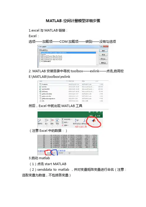
MATLAB-空间计量模型详细步骤1.excel与MATLAB链接:Excel:选项——加载项——COM加载项——转到——没有勾选项2. MATLAB安装目录中寻找toolbox——exlink——点击,启用宏E:\MATLAB\toolbox\exlink然后,Excel中就出现MATLAB工具(注意Excel中的数据:)3.启动matlab(1)点击start MATLAB(2)senddata to matlab ,并对变量矩阵变量进行命名(注意:选取变量为数值,不包括各变量)(data表中数据进行命名)(空间权重进行命名)(3)导入MATLAB中的两个矩阵变量就可以看见4.将elhorst和jplv7两个程序文件夹复制到MATLAB安装目录的toolbox文件夹5.设置路径:6.输入程序,得出结果T=30;N=46;W=norm(W1);y=A(:,3);x=A(:,[4,6]);xconstant=ones(N*T,1); [nobs K]=size(x);results=ols(y,[xconstant x]);vnames=strvcat('logcit','intercept','logp','logy');prt_reg(results,vnames,1);sige=results.sige*((nobs-K)/nobs);loglikols=-nobs/2*log(2*pi*sige)-1/(2*sige)*results.resid'*results.resid % The (robust)LM tests developed by ElhorstLMsarsem_panel(results,W,y,[xconstant x]); % (Robust) LM tests 解释附录:静态面板空间计量经济学一、OLS静态面板编程1、普通面板编程T=30;N=46;W=normw(W1);y=A(:,3);x=A(:,[4,6]);xconstant=ones(N*T,1);[nobs K]=size(x);results=ols(y,[xconstant x]);vnames=strvcat('logcit','intercept','logp','logy');prt_reg(results,vnames,1);sige=results.sige*((nobs-K)/nobs);loglikols=-nobs/2*log(2*pi*sige)-1/(2*sige)*results.resid'*results.resid % The (robust)LM tests developed by ElhorstLMsarsem_panel(results,W,y,[xconstant x]); % (Robust) LM tests2、空间固定OLS (spatial-fixed effects)T=30;N=46;W=normw(W1);y=A(:,3);x=A(:,[4,6]);xconstant=ones(N*T,1);[nobs K]=size(x);model=1;[ywith,xwith,meanny,meannx,meanty,meantx]=demean(y,x, N,T,model );results=ols(ywith,xwith);vnames=strvcat('logcit','logp','logy'); % should be changed if x is changedprt_reg(results,vnames);sfe=meanny-meannx*results.beta; % including the constant term yme = y - mean(y);et=ones(T,1);error=y-kron(et,sfe)-x*results.beta;rsqr1 = error'*error;rsqr2 = yme'*yme;FE_rsqr2 = 1.0 - rsqr1/rsqr2 % r-squared including fixed effectssige=results.sige*((nobs-K)/nobs);logliksfe=-nobs/2*log(2*pi*sige)-1/(2*sige)*results.resid'*results.residLMsarsem_panel(results,W,ywith,xwith); % (Robust) LM tests3、时期固定OLS(time-period fixed effects)T=30;N=46;W=normw(W1);y=A(:,3);x=A(:,[4,6]);xconstant=ones(N*T,1);[nobs K]=size(x);model=2;[ywith,xwith,meanny,meannx,meanty,meantx]=demean(y,x, N,T,model );results=ols(ywith,xwith);vnames=strvcat('logcit','logp','logy'); % should be changed if x is changedprt_reg(results,vnames);tfe=meanty-meantx*results.beta; % including the constant termyme = y - mean(y);en=ones(N,1);error=y-kron(tfe,en)-x*results.beta;rsqr1 = error'*error;rsqr2 = yme'*yme;FE_rsqr2 = 1.0 - rsqr1/rsqr2 % r-squared including fixed effectssige=results.sige*((nobs-K)/nobs);logliktfe=-nobs/2*log(2*pi*sige)-1/(2*sige)*results.resid'*results.residLMsarsem_panel(results,W,ywith,xwith); % (Robust) LM tests4、空间与时间双固定模型T=30;N=46;W=normw(W1);y=A(:,3);x=A(:,[4,6]);xconstant=ones(N*T,1);[nobs K]=size(x);model=3;[ywith,xwith,meanny,meannx,meanty,meantx]=demean(y,x, N,T,model );results=ols(ywith,xwith);vnames=strvcat('logcit','logp','logy'); % should be changed if x is changedprt_reg(results,vnames)en=ones(N,1);et=ones(T,1);intercept=mean(y)-mean(x)*results.beta;sfe=meanny-meannx*results.beta-kron(en,intercept);tfe=meanty-meantx*results.beta-kron(et,intercept);yme = y - mean(y);ent=ones(N*T,1);error=y-kron(tfe,en)-kron(et,sfe)-x*results.beta-kron(ent,intercept); rsqr1 = error'*error;rsqr2 = yme'*yme;FE_rsqr2 = 1.0 - rsqr1/rsqr2 % r-squared including fixed effects sige=results.sige*((nobs-K)/nobs);loglikstfe=-nobs/2*log(2*pi*sige)-1/(2*sige)*results.resid'*results.residLMsarsem_panel(results,W,ywith,xwith); % (Robust) LM tests二、静态面板SAR模型1、无固定效应(No fixed effects)T=30;N=46;W=normw(W1);y=A(:,[3]);x=A(:,[4,6]);for t=1:Tt1=(t-1)*N+1;t2=t*N;wx(t1:t2,:)=W*x(t1:t2,:);endxconstant=ones(N*T,1);[nobs K]=size(x);info.lflag=0;info.model=0;info.fe=0;results=sar_panel_FE(y,[xconstant x],W,T,info); vnames=strvcat('logcit','intercept','logp','logy');prt_spnew(results,vnames,1)% Print out effects estimatesspat_model=0;direct_indirect_effects_estimates(results,W,spat_model); panel_effects_sar(results,vnames,W);2、空间固定效应(Spatial fixed effects)T=30;N=46;W=normw(W1);y=A(:,[3]);x=A(:,[4,6]);for t=1:Tt1=(t-1)*N+1;t2=t*N;wx(t1:t2,:)=W*x(t1:t2,:);endxconstant=ones(N*T,1);[nobs K]=size(x);info.lflag=0;info.model=1;info.fe=0;results=sar_panel_FE(y,x,W,T,info);vnames=strvcat('logcit','logp','logy');prt_spnew(results,vnames,1)% Print out effects estimatesspat_model=0;direct_indirect_effects_estimates(results,W,spat_model);panel_effects_sar(results,vnames,W);3、时点固定效应(Time period fixed effects)T=30;N=46;W=normw(W1);y=A(:,[3]);x=A(:,[4,6]);for t=1:Tt1=(t-1)*N+1;t2=t*N;wx(t1:t2,:)=W*x(t1:t2,:);endxconstant=ones(N*T,1);[nobs K]=size(x);info.lflag=0; % required for exact resultsinfo.model=2;info.fe=0; % Do not print intercept and fixed effects; use info.fe=1 to turn onresults=sar_panel_FE(y,x,W,T,info);vnames=strvcat('logcit','logp','logy');prt_spnew(results,vnames,1)% Print out effects estimatesspat_model=0;direct_indirect_effects_estimates(results,W,spat_model);panel_effects_sar(results,vnames,W);4、双固定效应(Spatial and time period fixed effects)T=30;N=46;W=normw(W1);y=A(:,[3]);x=A(:,[4,6]);for t=1:Tt1=(t-1)*N+1;t2=t*N;wx(t1:t2,:)=W*x(t1:t2,:);endxconstant=ones(N*T,1);[nobs K]=size(x);info.lflag=0; % required for exact resultsinfo.model=3;info.fe=0; % Do not print intercept and fixed effects; use info.fe=1 to turn onresults=sar_panel_FE(y,x,W,T,info);vnames=strvcat('logcit','logp','logy');prt_spnew(results,vnames,1)% Print out effects estimatesspat_model=0;direct_indirect_effects_estimates(results,W,spat_model);panel_effects_sar(results,vnames,W);三、静态面板SDM模型1、无固定效应(No fixed effects)T=30;N=46;W=normw(W1);y=A(:,[3]);x=A(:,[4,6]);for t=1:Tt1=(t-1)*N+1;t2=t*N;wx(t1:t2,:)=W*x(t1:t2,:);endxconstant=ones(N*T,1);[nobs K]=size(x);info.lflag=0;info.model=0;info.fe=0;results=sar_panel_FE(y,[xconstant x wx],W,T,info);vnames=strvcat('logcit','intercept','logp','logy','W*logp','W*l ogy');prt_spnew(results,vnames,1)% Print out effects estimatesspat_model=1;direct_indirect_effects_estimates(results,W,spat_model);panel_effects_sdm(results,vnames,W);2、空间固定效应(Spatial fixed effects)T=30;N=46;W=normw(W1);y=A(:,[3]);x=A(:,[4,6]);for t=1:Tt1=(t-1)*N+1;t2=t*N;wx(t1:t2,:)=W*x(t1:t2,:);endxconstant=ones(N*T,1);[nobs K]=size(x);info.lflag=0; % required for exact resultsinfo.model=1;info.fe=0; % Do not print intercept and fixed effects; use info.fe=1 to turn onresults=sar_panel_FE(y,[x wx],W,T,info);vnames=strvcat('logcit','logp','logy','W*logp','W*logy');prt_spnew(results,vnames,1)% Print out effects estimatesspat_model=1;direct_indirect_effects_estimates(results,W,spat_model);panel_effects_sdm(results,vnames,W);3、时点固定效应(Time period fixed effects)T=30;N=46;W=norm(W1);y=A(:,[3]);x=A(:,[4,6]);for t=1:Tt1=(t-1)*N+1;t2=t*N;wx(t1:t2,:)=W*x(t1:t2,:);endxconstant=ones(N*T,1);[nobs K]=size(x);info.lflag=0; % required for exact resultsinfo.model=2;info.fe=0; % Do not print intercept and fixed effects; use info.fe=1 to turn on% New routines to calculate effects estimatesresults=sar_panel_FE(y,[x wx],W,T,info);vnames=strvcat('logcit','logp','logy','W*logp','W*logy');% Print out coefficient estimatesprt_spnew(results,vnames,1)% Print out effects estimatesspat_model=1;direct_indirect_effects_estimates(results,W,spat_model);panel_effects_sdm(results,vnames,W)4、双固定效应(Spatial and time period fixed effects)T=30;N=46;W=normw(W1);y=A(:,[3]);x=A(:,[4,6]);for t=1:Tt1=(t-1)*N+1;t2=t*N;wx(t1:t2,:)=W*x(t1:t2,:);endxconstant=ones(N*T,1);[nobs K]=size(x);info.bc=0;info.lflag=0; % required for exact resultsinfo.model=3;info.fe=0; % Do not print intercept and fixed effects; use info.fe=1 to turn onresults=sar_panel_FE(y,[x wx],W,T,info);vnames=strvcat('logcit','logp','logy','W*logp','W*logy');prt_spnew(results,vnames,1)% Print out effects estimatesspat_model=1;direct_indirect_effects_estimates(results,W,spat_model);panel_effects_sdm(results,vnames,W)wald test spatial lag% Wald test for spatial Durbin model against spatial lagmodelbtemp=results.parm;varcov=results.cov;Rafg=zeros(K,2*K+2);for k=1:KRafg(k,K+k)=1; % R(1,3)=0 and R(2,4)=0;endWald_spatial_lag=(Rafg*btemp)'*inv(Rafg*varcov*Rafg')*Raf g*btemp prob_spatial_lag=1-chis_cdf (Wald_spatial_lag, K) wald test spatial error% Wald test spatial Durbin model against spatial error model R=zeros(K,1);for k=1:KR(k)=btemp(2*K+1)*btemp(k)+btemp(K+k); % k changed in 1,7/12/2010% R(1)=btemp(5)*btemp(1)+btemp(3);% R(2)=btemp(5)*btemp(2)+btemp(4);endRafg=zeros(K,2*K+2);for k=1:KRafg(k,k) =btemp(2*K+1); % k changed in 1, 7/12/2010Rafg(k,K+k) =1;Rafg(k,2*K+1)=btemp(k);% Rafg(1,1)=btemp(5);Rafg(1,3)=1;Rafg(1,5)=btemp(1);% Rafg(2,2)=btemp(5);Rafg(2,4)=1;Rafg(2,5)=btemp(2);endWald_spatial_error=R'*inv(Rafg*varcov*Rafg')*Rprob_spatial_error=1-chis_cdf (Wald_spatial_error,K)LR test spatial lagresultssar=sar_panel_FE(y,x,W,T,info);LR_spatial_lag=-2*(resultssar.lik-results.lik)prob_spatial_lag=1-chis_cdf (LR_spatial_lag,K)LR test spatial errorresultssem=sem_panel_FE(y,x,W,T,info);LR_spatial_error=-2*(resultssem.lik-results.lik)prob_spatial_error=1-chis_cdf (LR_spatial_error,K)5、空间随机效应与时点固定效应模型T=30;N=46;W=normw(W1);y=A(:,[3]);x=A(:,[4,6]);for t=1:Tt1=(t-1)*N+1;t2=t*N;wx(t1:t2,:)=W*x(t1:t2,:);endxconstant=ones(N*T,1);[nobs K]=size(x);[ywith,xwith,meanny,meannx,meanty,meantx]=demean(y,[x wx],N,T,2); % 2=time dummiesinfo.model=1;results=sar_panel_RE(ywith,xwith,W,T,info);prt_spnew(results,vnames,1)spat_model=1;direct_indirect_effects_estimates(results,W,spat_model);panel_effects_sdm(results,vnames,W)wald test spatial lagbtemp=results.parm(1:2*K+2);varcov=results.cov(1:2*K+2,1:2*K+2);Rafg=zeros(K,2*K+2);for k=1:KRafg(k,K+k)=1; % R(1,3)=0 and R(2,4)=0;endWald_spatial_lag=(Rafg*btemp)'*inv(Rafg*varcov*Rafg')*Raf g*btempprob_spatial_lag= 1-chis_cdf (Wald_spatial_lag, K)wald test spatial errorR=zeros(K,1);for k=1:KR(k)=btemp(2*K+1)*btemp(k)+btemp(K+k); % k changed in 1,7/12/2010% R(1)=btemp(5)*btemp(1)+btemp(3);% R(2)=btemp(5)*btemp(2)+btemp(4);endRafg=zeros(K,2*K+2);for k=1:KRafg(k,k) =btemp(2*K+1); % k changed in 1, 7/12/2010 Rafg(k,K+k) =1;Rafg(k,2*K+1)=btemp(k);% Rafg(1,1)=btemp(5);Rafg(1,3)=1;Rafg(1,5)=btemp(1);% Rafg(2,2)=btemp(5);Rafg(2,4)=1;Rafg(2,5)=btemp(2);endWald_spatial_error=R'*inv(Rafg*varcov*Rafg')*Rprob_spatial_error= 1-chis_cdf (Wald_spatial_error,K)LR test spatial lagresultssar=sar_panel_RE(ywith,xwith(:,1:K),W,T,info);LR_spatial_lag=-2*(resultssar.lik-results.lik)prob_spatial_lag=1-chis_cdf (LR_spatial_lag,K)LR test spatial errorresultssem=sem_panel_RE(ywith,xwith(:,1:K),W,T,info);LR_spatial_error=-2*(resultssem.lik-results.lik)prob_spatial_error=1-chis_cdf (LR_spatial_error,K)四、静态面板SEM模型1、无固定效应(No fixed effects)T=30;N=46;W=normw(W1);y=A(:,[3]);x=A(:,[4,6]);for t=1:Tt1=(t-1)*N+1;t2=t*N;wx(t1:t2,:)=W*x(t1:t2,:);endxconstant=ones(N*T,1);[nobs K]=size(x);info.lflag=0;info.model=0;info.fe=0;results=sem_panel_FE(y,[xconstant x],W,T,info);vnames=strvcat('logcit','intercept','logp','logy');prt_spnew(results,vnames,1)% Print out effects estimatesspat_model=0;direct_indirect_effects_estimates(results,W,spat_model); panel_effects_sar(results,vnames,W);2、空间固定效应(Spatial fixed effects)T=30;N=46;W=normw(W1);y=A(:,[3]);x=A(:,[4,6]);for t=1:Tt1=(t-1)*N+1;t2=t*N;wx(t1:t2,:)=W*x(t1:t2,:);endxconstant=ones(N*T,1);[nobs K]=size(x);info.lflag=0;info.model=1;info.fe=0;results=sem_panel_FE(y,x,W,T,info);vnames=strvcat('logcit','logp','logy');prt_spnew(results,vnames,1)% Print out effects estimatesspat_model=0;direct_indirect_effects_estimates(results,W,spat_model); panel_effects_sar(results,vnames,W);3、时点固定效应(Time period fixed effects)T=30;N=46;W=normw(W1);y=A(:,[3]);x=A(:,[4,6]);for t=1:Tt1=(t-1)*N+1;t2=t*N;wx(t1:t2,:)=W*x(t1:t2,:);endxconstant=ones(N*T,1);[nobs K]=size(x);info.lflag=0; % required for exact resultsinfo.model=2;info.fe=0; % Do not print intercept and fixed effects; use info.fe=1 to turn onresults=sem_panel_FE(y,x,W,T,info);vnames=strvcat('logcit','logp','logy');prt_spnew(results,vnames,1)% Print out effects estimatesspat_model=0;direct_indirect_effects_estimates(results,W,spat_model);panel_effects_sar(results,vnames,W);4、双固定效应(Spatial and time period fixed effects)T=30;N=46;W=normw(W1);y=A(:,[3]);x=A(:,[4,6]);for t=1:Tt1=(t-1)*N+1;t2=t*N;wx(t1:t2,:)=W*x(t1:t2,:);endxconstant=ones(N*T,1);[nobs K]=size(x);info.lflag=0; % required for exact resultsinfo.model=3;info.fe=0; % Do not print intercept and fixed effects; use info.fe=1 to turn onresults=sem_panel_FE(y,x,W,T,info);vnames=strvcat('logcit','logp','logy');prt_spnew(results,vnames,1)% Print out effects estimatesspat_model=0;direct_indirect_effects_estimates(results,W,spat_model); panel_effects_sar(results,vnames,W);五、静态面板SDEM模型1、无固定效应(No fixed effects)T=30;N=46;W=normw(W1);y=A(:,[3]);x=A(:,[4,6]);。

Matlab技术经济学应用引言:技术经济学是一门研究科技创新与经济发展之间相互关系的学科,而Matlab作为一种强大的数值计算和科学编程语言,被广泛应用于技术经济学领域。
本文将重点探讨Matlab在技术经济学中的应用,着重介绍其在经济评估、金融模型、企业决策等方面的应用。
一、经济评估1.1 投资成本分析在进行经济评估时,投资成本分析是一个重要的步骤。
Matlab可以帮助分析人员通过数学模型计算出投资成本,并进行灵活的调整和优化。
例如,可以使用Matlab编写一个程序,基于现金流量贴现法(NPV)来计算投资项目的净现值。
通过调整输入参数,可以模拟不同情况下的投资成本,并找到最优方案。
1.2 效益评估Matlab也可以用于效益评估,即对投资项目的经济效益进行分析。
例如,可以使用Matlab编写一个程序来计算投资项目的内部收益率(IRR),并评估其可行性和盈利能力。
通过在程序中引入不同的输入变量,可以进行灵活的模拟和分析,帮助决策者做出科学的投资决策。
二、金融模型2.1 期权定价模型期权定价是金融领域中的一个重要问题,Matlab提供了强大的数学计算功能,可以用于构建和求解各种期权定价模型。
例如,可以使用Matlab编写程序,基于布莱克-斯科尔斯(Black-Scholes)模型来估计欧式期权的价格。
通过调整输入参数,可以对不同情况下的期权价格进行计算和分析。
2.2 风险管理模型金融市场中存在着各种风险,如市场风险、信用风险等。
Matlab可以用于构建和求解各种风险管理模型,以帮助投资者进行风险评估和管理。
例如,可以使用Matlab编写程序,基于Value at Risk(VaR)模型来评估投资组合的风险水平,并制定相应的风险管理策略。
三、企业决策3.1 供应链优化供应链管理是现代企业中的一个重要问题,而Matlab可以帮助企业进行供应链优化。
例如,可以使用Matlab编写程序,基于线性规划模型来优化供应链网络的布局和物流运输方案。
在Matlab中进行模型建立和参数估计引言在科学研究和工程实践中,建立数学模型并通过参数估计对模型进行优化是常见的任务。
Matlab作为一种功能强大的数学计算工具,提供了丰富的函数和工具箱,可以方便地进行模型建立和参数估计。
本文将介绍在Matlab中进行模型建立和参数估计的基本方法和技巧。
一、模型建立模型建立是构建一个能够描述实际问题的数学模型的过程。
在Matlab中,可以使用符号运算工具箱(Symbolic Math Toolbox)来定义符号变量和代数表达式,并利用这些符号变量和代数表达式构建模型。
例如,对于线性回归模型,可以使用符号变量定义输入变量和待估参数,并通过代数表达式构建模型方程。
除了使用符号运算工具箱,Matlab还提供了许多其他工具箱和函数来进行模型建立。
例如,Curve Fitting Toolbox可以用于拟合曲线和表面,System Identification Toolbox可以用于系统建模和参数估计等。
这些工具箱和函数提供了丰富的方法和算法来支持各种类型的模型建立。
二、参数估计参数估计是通过观测数据来估计模型中的未知参数的过程。
在Matlab中,可以使用最小二乘法(Least Squares)或最大似然估计(Maximum Likelihood Estimation)等方法进行参数估计。
最小二乘法是一种常用的参数估计方法,通过最小化观测数据与模型预测值之间的误差平方和来估计参数。
在Matlab中,可以使用lsqcurvefit函数或最小二乘曲线拟合工具箱(Curve Fitting Toolbox)中的相关函数来进行最小二乘估计。
这些函数可以根据用户提供的模型函数、初始参数值和观测数据进行参数估计,并返回估计的参数值和相应的拟合误差等信息。
最大似然估计是一种统计推断方法,通过估计参数使得观测数据的出现概率最大化。
在Matlab中,可以使用mle函数或Probability Distribution Fitting工具箱中的相关函数进行最大似然估计。
matlab中ma参数估计Estimating parameters in a moving average (MA) model in Matlab can be a complex but essential task in time series analysis. The MA model is commonly used to represent the stochastic process of a time series, with random noise being incorporated into the model through the MA parameters. By accurately estimating these parameters, analysts can better understand and predict the behavior of the time series data.在Matlab中估计移动平均(MA)模型中的参数可能是时间序列分析中一个复杂但必要的任务。
MA模型通常用于表示时间序列的随机过程,通过MA参数将随机噪声纳入模型中。
通过准确估计这些参数,分析师可以更好地了解和预测时间序列数据的行为。
One way to estimate MA parameters in Matlab is through maximum likelihood estimation. This method involves finding the values of the MA parameters that maximize the likelihood function, which measures how well the model explains the observed data. By iteratively adjusting the parameter values to maximize the likelihood, analysts can arrive at estimates that best fit the data.在Matlab中估计MA参数的一种方法是通过最大似然估计。

Matlab中常用的最小二乘(LS)估计方法是一种常见的参数估计方法。
在统计分析和数据建模中,LS估计可以帮助我们估计出模型参数的最佳值,以最好地拟合观测数据。
本文将对Matlab中LS估计的估计值进行深度和广度的探讨,以帮助读者更好地理解和应用这一估计方法。
1. LS估计的原理和应用LS估计的原理是通过最小化观测数据与模型预测值之间的残差平方和,来找到最适合的模型参数。
在Matlab中,可以使用“lsqcurvefit”或者“polyfit”等函数来实现LS估计的应用。
其中,“lsqcurvefit”适用于非线性模型参数的估计,而“polyfit”适用于多项式拟合模型的参数估计。
2. Matlab中LS估计的具体实现在Matlab中,可以通过编写自定义的拟合模型函数来实现LS估计。
首先要定义模型函数的形式,然后使用“lsqcurvefit”函数进行参数估计。
通过调用该函数,并传入观测数据和初始参数的估计值,可以得到LS估计的最优参数值。
3. LS估计的优缺点LS估计作为一种常见的参数估计方法,具有很多优点。
它可以用于各种类型的模型拟合,包括线性和非线性模型。
LS估计还可以通过加权最小二乘法进行改进,适应不同方差的观测数据。
然而,LS估计也存在一些缺点,例如对异常值敏感,以及可能出现多重共线性的问题。
4. 个人观点和理解在我看来,LS估计作为一种经典的参数估计方法,在实际应用中具有广泛的适用性和灵活性。
在Matlab中,利用其强大的数据处理和优化工具,可以更轻松地实现LS估计,并通过可视化工具来验证拟合效果。
然而,需要注意的是在应用LS估计时,要结合实际问题特点,对参数估计结果进行适当的解释和评估。
总结回顾:通过本文的介绍,读者对Matlab中LS估计的估计值应该有了更深入的理解。
通过对LS估计的原理、实现方法、优缺点和个人观点的探讨,我们可以更好地把握LS估计的特点和适用范围。
在实际应用中,希望读者能够充分利用Matlab的工具和LS估计方法,为数据建模和分析提供更准确、可靠的结果。

如何使用Matlab进行空间数据分析引言:随着科技的不断进步,我们生活的这个世界正变得越来越数字化。
在这个数字化时代中,收集和分析空间数据变得越来越重要。
作为一种功能强大的数学软件,Matlab可以帮助我们进行空间数据分析。
本文将介绍如何使用Matlab进行空间数据分析的基本方法和技巧。
一、数据准备在进行空间数据分析之前,我们需要准备相应的数据。
空间数据可以包括地理坐标、地形图、气象数据等等。
在Matlab中,我们可以通过多种方式导入这些数据。
比如,我们可以使用地图坐标系统进行坐标转换,将不同的空间数据调整到同一个坐标系统下,方便后续的分析。
二、数据可视化在进行空间数据分析之前,我们需要对数据进行可视化。
Matlab提供了丰富的绘图函数和工具箱,可以帮助我们将空间数据映射为图像。
例如,我们可以使用绘图函数plot3将三维坐标点绘制在三维坐标系的图中。
此外,我们还可以使用绘图函数contour和surf对二维或三维数据进行等值线图或曲面图的可视化。
三、空间插值空间插值是一种将离散的空间数据点通过插值算法生成连续的空间数据场的方法。
Matlab提供了许多插值方法(如最近邻插值、反距离加权插值、克里金插值等),可以根据具体情况选择合适的插值方法。
通过空间插值,我们可以预测未知位置的值,并通过等值曲线图或等值面图对连续的空间数据进行可视化。
四、空间统计分析在对空间数据进行分析时,我们通常需要了解数据的特征和变异性。
Matlab提供了丰富的统计函数和工具箱,可以帮助我们计算空间数据的统计指标,如均值、方差、标准差等。
此外,我们还可以使用相关性分析和半变异函数来揭示空间数据之间的关系和变化规律。
五、空间回归分析当我们需要了解空间数据的影响因素及其空间分布规律时,可以使用空间回归分析。
Matlab提供了相关的统计工具箱,可以进行空间回归分析,并生成相应的回归模型。
通过空间回归分析,我们可以找出重要的自变量,并预测因变量在空间上的分布。
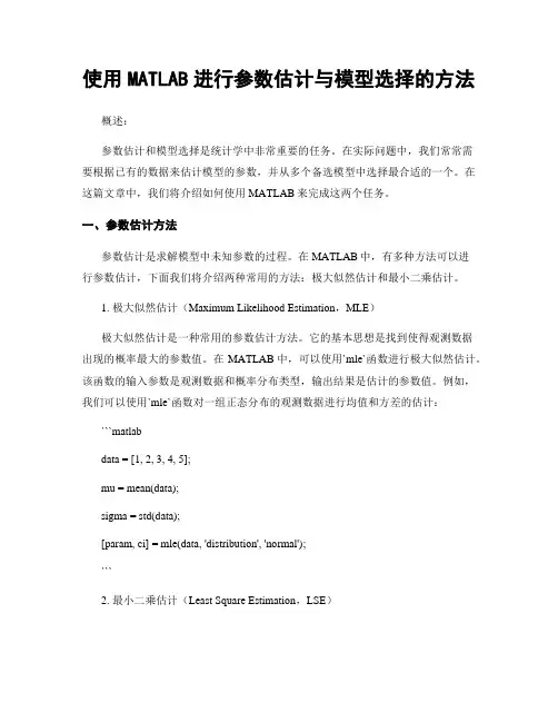
使用MATLAB进行参数估计与模型选择的方法概述:参数估计和模型选择是统计学中非常重要的任务。
在实际问题中,我们常常需要根据已有的数据来估计模型的参数,并从多个备选模型中选择最合适的一个。
在这篇文章中,我们将介绍如何使用MATLAB来完成这两个任务。
一、参数估计方法参数估计是求解模型中未知参数的过程。
在MATLAB中,有多种方法可以进行参数估计,下面我们将介绍两种常用的方法:极大似然估计和最小二乘估计。
1. 极大似然估计(Maximum Likelihood Estimation,MLE)极大似然估计是一种常用的参数估计方法。
它的基本思想是找到使得观测数据出现的概率最大的参数值。
在MATLAB中,可以使用`mle`函数进行极大似然估计。
该函数的输入参数是观测数据和概率分布类型,输出结果是估计的参数值。
例如,我们可以使用`mle`函数对一组正态分布的观测数据进行均值和方差的估计:```matlabdata = [1, 2, 3, 4, 5];mu = mean(data);sigma = std(data);[param, ci] = mle(data, 'distribution', 'normal');```2. 最小二乘估计(Least Square Estimation,LSE)最小二乘估计是一种广泛应用的参数估计方法,特别适用于线性回归模型。
它的基本思想是通过最小化预测值与观测值之间的差异来估计参数。
在MATLAB中,可以使用`lsqcurvefit`函数进行最小二乘估计。
该函数的输入参数是待拟合的函数模型、观测数据和初始参数值,输出结果是估计的参数值。
例如,我们可以使用`lsqcurvefit`函数对一组带有噪声的正弦函数进行参数估计:```matlabx = 0:0.1:pi;y = sin(x) + randn(size(x))*0.1;fun = @(p,x) p(1)*sin(p(2)*x);p0 = [1, 1];p = lsqcurvefit(fun, p0, x, y);```二、模型选择方法模型选择是从多个备选模型中选择最合适的一个。
使用MATLAB进行参数估计与模型选择的方法在MATLAB中,有多种方法可以进行参数估计与模型选择,其中包括最小二乘法、最大似然估计、贝叶斯统计和交叉验证。
最小二乘法:最小二乘法是一种常见的参数估计方法,适用于线性模型。
在MATLAB中,可以使用`polyfit`函数进行最小二乘法估计。
该函数采用原始数据点的坐标和多项式的次数作为输入,并返回多项式系数。
```matlabx=[1,2,3,4,5];y=[1,4,9,14,24];degree = 2;coefficients = polyfit(x, y, degree);```最大似然估计:最大似然估计是一种参数估计方法,通过最大化观测数据的可能性来估计参数。
在MATLAB中,可以使用`mle`函数进行最大似然估计。
该函数要求用户提供一个自定义的似然函数,该函数将根据参数估计观测数据的可能性。
```matlabx=[1,2,3,4,5];startingVals = [0, 1];estimates = mle(y, 'pdf', likelihoodFunc, 'start', startingVals);```贝叶斯统计:贝叶斯统计是一种基于概率的模型选择方法,通过计算后验概率来进行模型选择和参数估计。
在MATLAB中,可以使用`bayeslm`函数进行贝叶斯线性回归的模型选择。
该函数采用原始数据点的坐标和响应变量作为输入,并返回具有最高后验概率的线性回归模型。
```matlabx=[1,2,3,4,5];y=[1,4,9,14,24];model = bayeslm(x, y);```交叉验证:交叉验证是一种常用的模型选择方法,通过将数据集分成训练集和测试集来评估模型的性能。
在MATLAB中,可以使用`cvpartition`函数将数据集分成训练集和测试集。
然后,可以使用交叉验证来选择模型,并使用测试集进行性能评估。
matlab vasicek模型参数估计Matlab Vasicek模型参数估计Vasicek模型是一种用于描述利率市场的数学模型,它是由捷克经济学家Ole Hagan Vasicek于1977年提出的。
该模型是基于随机微分方程的,可以用于估计利率的未来走势。
在本文中,将介绍如何使用Matlab进行Vasicek模型的参数估计。
我们需要收集利率数据,以便对Vasicek模型进行参数估计。
这些数据可以从金融数据提供商或金融数据库中获取,如Yahoo Finance或Bloomberg。
在本文中,我们将使用Matlab自带的数据集“Datafeed Toolbox”中的美国国债收益率数据作为例子。
在Matlab中,我们可以使用“datafeed”函数来获取美国国债收益率数据。
首先,我们需要指定数据的起始日期和结束日期,并选择适当的利率期限。
例如,我们可以选择10年期的美国国债收益率数据。
然后,我们可以使用“fetch”函数从数据源获取数据。
获取到的数据将被存储在一个表格中,方便后续处理和分析。
在得到利率数据后,我们可以使用Vasicek模型进行参数估计。
Vasicek模型的基本形式如下:dr = a(b - r)dt + σdW其中,dr是利率的变化,a是回归系数,b是利率的均值,r是当前的利率,σ是波动率,dW是布朗运动。
我们的目标是根据观测到的利率数据,估计出模型中的参数a、b和σ。
在Matlab中,我们可以使用最小二乘法来估计Vasicek模型的参数。
首先,我们需要对模型进行离散化,将其转化为差分方程。
然后,我们可以使用“lsqcurvefit”函数来拟合模型,并得到参数的估计值。
具体地说,我们可以将Vasicek模型离散化为以下形式:r(t+Δt) = r(t) + a(b - r(t))Δt + σ√Δtε其中,r(t)是第t期的利率,Δt是时间间隔,ε是一个标准正态分布随机变量。
我们可以通过最小二乘法来拟合模型,找到最优的参数估计值。
Matlab程序命令(四)数据处理及空间自回归模型参数估计一、教材实例Matlab操作过程(注意:在进行空间计量模型参数估计时,要把空间计量软件包jplv7和fanzuan、lYhbzh函数添加到Matlab程序文件夹中,否则,所有与Matlab相关的程序、函数等都能够被Matlab识别并使用)%空间自回归模型设立%移项、矩阵变换%估计结果(一)构造变量矩阵y=[42;37;30;26;30;37;42] %7行1列矩阵x=[10,30;20,20;30,10;50,0;30,10;20,20;10,30] %7行2列矩阵(二)构建已经行标准化的空间权重矩阵W=zeros(7) %建立7×7零矩阵W(1,2)=1 %赋W第1行第2列为1的值W(2,1)=0.5 %赋W第2行第1列为0.5的值W(2,3) =0.5 %赋W第2行第3列为0.5的值W(3,2) =0.5 %赋W第3行第2列为0.5的值W(3,4) =0.5 %赋W第3行第4列为0.5的值W(4,3) =0.5 %赋W第4行第3列为0.5的值W(4,5) =0.5 %赋W第4行第5列为0.5的值W(5,4) =0.5 %赋W第5行第4列为0.5的值W(5,6) =0.5 %赋W第5行第6列为0.5的值W(6,5) =0.5 %赋W第6行第5列为0.5的值W(6,7) =0.5 %赋W第6行第7列为0.5的值W(7,6) =1 %赋W第7行第6列为1的值(三)估计空间自回归模型Matlab程序命令results = sar(y,x,W) %估计估计空间自回归模型参数prt(results) %格式化二、教材实例(续)(一)引进函数lyhbzh的Matlab程序命令A=zeros(7); %生成7×7阶0矩阵AA(1,2)=1; %A矩阵中第1行第2列元素为1A(2,1)=1; %A矩阵中第2行第1列元素为1A(2,3)=1; %A矩阵中第2行第3列元素为1A(3,2)=1; %A矩阵中第3行第2列元素为1A(3,4)=1; %A矩阵中第3行第4列元素为1A(4,3)=1; %A矩阵中第4行第3列元素为1A(4,5)=1; %A矩阵中第4行第5列元素为1A(5,4)=1; %A矩阵中第5行第4列元素为1A(5,6)=1; %A矩阵中第5行第6列元素为1A(6,5)=1; %A矩阵中第6行第5列元素为1A(6,7)=1; %A矩阵中第6行第7列元素为1A(7,6)=1; %A矩阵中第7行第6列元素为1W=lyhbzh(A); %对矩阵A行标准化y=[42;37;30;26;30;37;42]; %出行时间的列向量x1=[10;20;30;50;30;20;10]; %人口密度的列向量x2=[30;20;10;0;10;20;30]; %到中央商务区的距离的列向量x=horzcat(x1,x2); %x1和x2并列排列vnames=strvcat('y','x1','x2'); %对变量命名results =sar(y,x,W); %估计空间自回归模型的参数prt(results,vnames) %对估计空间自回归模型的参数进行格式化%以下是计算y1,y2和dy的Matlab程序命令I=eye(7); %生成7×7阶单位矩阵B=inv(I-0.642975*W) %计算y1=B*x*[0.135137;0.56] %计算y1x(2,1)=40; %把x中第2行第1列的元素改为40y2=B*x*[0.135137;0.56] %计算y2dy=y2-y1 %计算dy%下面给出具体的操作步骤第一步:构建邻域空间权重矩阵A=zeros(7); %生成7×7阶0矩阵AA(1,2)=1; %A矩阵中第1行第2列元素为1A(2,1)=1; %A矩阵中第2行第1列元素为1A(2,3)=1; %A矩阵中第2行第3列元素为1A(3,2)=1; %A矩阵中第3行第2列元素为1A(3,4)=1; %A矩阵中第3行第4列元素为1A(4,3)=1; %A矩阵中第4行第3列元素为1A(4,5)=1; %A矩阵中第4行第5列元素为1A(5,4)=1; %A矩阵中第5行第4列元素为1A(5,6)=1; %A矩阵中第5行第6列元素为1A(6,5)=1; %A矩阵中第6行第5列元素为1A(6,7)=1; %A矩阵中第6行第7列元素为1A(7,6)=1; %A矩阵中第7行第6列元素为1A=0 1 0 0 0 0 01 0 1 0 0 0 0 0 1 0 1 0 0 0 0 0 1 0 1 0 0 0 0 0 1 0 1 0 0 0 0 0 1 0 1 0 0 0 0 0 1 0第二步:A进行行标准化W=hbzh(A)W =0 1.0000 0 0 0 0 00.5000 0 0.5000 0 0 0 0 0 0.5000 0 0.5000 0 0 0 0 0 0.5000 0 0.5000 0 0 0 0 0 0.5000 0 0.5000 0 0 0 0 0 0.5000 0 0.5000 0 0 0 0 0 1.0000 0第三步:构建y,x变量y=[42;37;30;26;30;37;42] %出行时间y =42373026303742x1=[10;20;30;50;30;20;10] %人口密度x1 =10203050302010x2=[30;20;10;0;10;20;30] %到中央商务区的距离x2 =302010102030x=horzcat(x1,x2) %x1和x2并列排x =10 3020 2030 1050 030 1020 2010 30第四步:空间自回归模型参数估计空间自回归模型:变换为:results =sar(y,x,W);prt(results)Spatial autoregressive Model EstimatesR-squared = 0.9999Rbar-squared = 0.9999sigma^2 = 0.0038Nobs, Nvars = 7, 2log-likelihood = 10.844689# of iterations = 18min and max rho = -1.0000, 1.0000total time in secs = 1.0610time for lndet = 0.1250time for t-stats = 0.2340time for x-impacts = 0.1400# draws x-impacts = 1000Pace and Barry, 1999 MC lndet approximation usedorder for MC appr = 50iter for MC appr = 30*************************************************************** Variable Coefficient Asymptot t-stat z-probabilityvariable 1 0.135137 14.939012 0.000000variable 2 0.561200 37.497156 0.000000rho 0.642975 46.232379 0.000000Direct Coefficient t-stat t-prob lower 01 upper 99 variable 1 0.181608 20.357543 0.000000 0.154298 0.205780 variable 2 0.754111 101.842843 0.000000 0.733892 0.774507Indirect Coefficient t-stat t-prob lower 01 upper 99 variable 1 0.196727 93.940264 0.000000 0.189259 0.201305 variable 2 0.818219 31.127774 0.000000 0.750695 0.891202Total Coefficient t-stat t-prob lower 01 upper 99 variable 1 0.378336 35.548934 0.000000 0.343579 0.404899 variable 2 1.572331 80.780336 0.000000 1.523822 1.633477第五步:计算=0.642975;A= %单位矩阵A=eye(7) %单位矩阵A =1 0 0 0 0 0 00 1 0 0 0 0 00 0 1 0 0 0 00 0 0 1 0 0 00 0 0 0 1 0 00 0 0 0 0 1 00 0 0 0 0 0 1>> B=inv(A-0.642975*W) %计算B =1.3057 0.9509 0.3463 0.1263 0.0467 0.0189 0.0061 0.4754 1.4788 0.5386 0.1965 0.0726 0.0294 0.0095 0.1732 0.5386 1.3290 0.4849 0.1792 0.0726 0.0234 0.0632 0.1965 0.4849 1.3118 0.4849 0.1965 0.0632 0.0234 0.0726 0.1792 0.4849 1.3290 0.5386 0.1732 0.0095 0.0294 0.0726 0.1965 0.5386 1.4788 0.4754 0.0061 0.0189 0.0467 0.1263 0.3463 0.9509 1.3057D=B*0.135137D =0.1764 0.1285 0.0468 0.0171 0.0063 0.0026 0.0008 0.0642 0.1998 0.0728 0.0266 0.0098 0.0040 0.0013 0.0234 0.0728 0.1796 0.0655 0.0242 0.0098 0.0032 0.0085 0.0266 0.0655 0.1773 0.0655 0.0266 0.0085 0.0032 0.0098 0.0242 0.0655 0.1796 0.0728 0.0234 0.0013 0.0040 0.0098 0.0266 0.0728 0.1998 0.0642 0.0008 0.0026 0.0063 0.0171 0.0468 0.1285 0.1764trace(D)/7 %矩阵D的迹的均值,ans =0.1842则y1=B*x*[0.135137;0.56]yy1=B*xyy1 =50.6213 62.679163.1772 50.824983.6830 33.2029103.8061 21.348683.6830 33.202963.1772 50.824950.6213 62.6791y1 =yy1*[0.135137;0.56]y1 =41.941136.999529.902325.983329.902336.999541.9411第五步:计算R2人口密度增加一倍y2=B*x*[0.135137;0.56]y2 =44.511040.996431.358026.514430.098637.079141.9923dy=y2-y1dy =2.56993.99691.45570.53110.19630.07960.0512第六步:空间溢出效应的分解……人口密度变化对人们出行时间的直接效应和空间外溢效应效应平均值标准差t统计值直接效应0.1842空间外溢效应0.1943总效应0.3785W阶叠加直接空间外溢效应0.135137 0.135137 0.0000000.0869 0.000000 0.08690.0529 0.0319 0.02100.0359 0.000000 0.03590.0251 0.0107 0.01440.0148 0.000000 0.01480.0105 0.0039 0.00660.0062 0.000000 0.00620.3674 0.1816 0.1858当q=0,当=0.135137;=0.642975;当q=1=0.135137;=0.642975;当q=2=0.135137;=0.642975;当q=3=0.135137;=0.642975;当q=4=0.135137;=0.642975;当q=5=0.135137;=0.642975;当q=6=0.135137;=0.642975;当q=7=0.135137;=0.642975;第七步:传统回归模型results = ols(y,x);prt(results)Ordinary Least-squares EstimatesR-squared = 0.9652Rbar-squared = 0.9582sigma^2 = 1.6487Durbin-Watson = 2.5084Nobs, Nvars = 7, 2*************************************************************** Variable Coefficient t-statistic t-probabilityvariable 1 0.551292 26.714374 0.000001variable 2 1.249077 43.994071 0.000000y3=x*[0.551292;1.249077]y3 =42.985236.007429.029527.564629.029536.007442.9852计算R2人口密度增加一倍Y4=x*[0.551292;1.249077]y4=x*[0.551292;1.249077]y4 =42.985247.033229.029527.564629.029536.007442.9852ddy=y4-y3ddy =11.0258s1=B*0.135137s1 =0.1764 0.1285 0.0468 0.0171 0.0063 0.0026 0.0008 0.0642 0.1998 0.0728 0.0266 0.0098 0.0040 0.0013 0.0234 0.0728 0.1796 0.0655 0.0242 0.0098 0.0032 0.0085 0.0266 0.0655 0.1773 0.0655 0.0266 0.0085 0.0032 0.0098 0.0242 0.0655 0.1796 0.0728 0.02340.0013 0.0040 0.0098 0.0266 0.0728 0.1998 0.06420.0008 0.0026 0.0063 0.0171 0.0468 0.1285 0.1764ss1=s1*x1ss1 =6.84088.537611.308714.028011.30878.53766.8408s2=B*0.5612s2 =0.7328 0.5336 0.1943 0.0709 0.0262 0.0106 0.00340.2668 0.8299 0.3023 0.1103 0.0408 0.0165 0.00530.0972 0.3023 0.7459 0.2721 0.1006 0.0408 0.01310.0355 0.1103 0.2721 0.7362 0.2721 0.1103 0.03550.0131 0.0408 0.1006 0.2721 0.7459 0.3023 0.09720.0053 0.0165 0.0408 0.1103 0.3023 0.8299 0.26680.0034 0.0106 0.0262 0.0709 0.1943 0.5336 0.7328三、实例一安徽省财政收入的空间效应分析--基于地级市视角Matlab操作过程(注意:在进行空间计量模型参数估计时,要把空间计量软件包jplv7和fanzuan、lYhbzh函数添加到Matlab程序文件夹中,否则,所有与Matlab相关的程序、函数等都能够被Matlab识别并使用)(一)数据处理1.在EXcel中将所搜集到的2011、2012年安徽省经济数据进行处理,进行对数化后得到以下数据图1 2011年安徽省各市经济数据图2 2012年安徽省各市经济数据2.构建安徽省各市直线地理距离和领域的权重矩阵,矩阵如下。
matlab计量经济学辅导书
摘要:
1.MATLAB 简介
2.MATLAB 在计量经济学中的应用
3.MATLAB 计量经济学辅导书的作用
4.推荐的MATLAB 计量经济学辅导书
正文:
MATLAB 是一款广泛应用于科学计算和数据分析的软件,它的强大的功能和易于使用的特性使其成为许多学科领域的重要工具,其中包括计量经济学。
在计量经济学中,MATLAB 可以用于数据的处理和分析,模型的建立和估计,以及结果的图形化展示等。
它可以帮助我们更方便地进行数据处理,更准确地估计模型参数,更直观地展示结果,从而提高我们的研究效率和质量。
对于学习计量经济学的人来说,一本好的MATLAB 计量经济学辅导书是非常有帮助的。
它可以帮助我们更好地理解MATLAB 在计量经济学中的应用,掌握MATLAB 的使用技巧,提高我们的研究能力。
在这里,我推荐几本MATLAB 计量经济学辅导书。
首先是《MATLAB 在计量经济学中的应用》,这本书详细介绍了MATLAB 在计量经济学中的各种应用,包括数据的处理和分析,模型的建立和估计等。
其次是《MATLAB 编程技巧与计量经济学实战》,这本书不仅介绍了MATLAB 的使用技巧,还通过实际的计量经济学问题,讲解了如何使用MATLAB 进行研究。
总的来说,MATLAB 在计量经济学中的应用非常广泛,而一本好的
MATLAB 计量经济学辅导书可以大大提高我们的研究效率和质量。
Matlab与经济学模型的应用技巧总结目前,计算机技术在各个领域的应用日益普及。
在经济学领域,诸如财务分析、市场预测、经济模型等都离不开计算机软件的辅助。
其中,Matlab作为一款专业的数值计算和数据分析工具,为经济学模型的构建和分析提供了强有力的支持。
在本文中,我们将从不同的角度总结和探讨Matlab在经济学模型应用中的技巧和方法。
一、数据处理与分析在经济学研究中,数据处理与分析是非常重要的一环。
Matlab提供了强大的数据操作和处理函数,可以方便地进行数据的导入、整理和转换。
比如,我们可以使用csvread函数将.csv格式的数据导入到Matlab中,利用table和array2table函数将数据转换为表格形式,并通过table的列操作实现数据的筛选和整理。
在数据分析方面,Matlab提供了多种统计工具和函数,如统计量计算、数据可视化等。
对于经济学的时间序列分析,我们可以使用Matlab中的time series对象进行建模和分析。
此外,Matlab还提供了强大的绘图功能,可以轻松地生成各种图表,如线图、柱状图、散点图等,方便经济学研究者对数据进行可视化展示和分析。
二、经济模型的建立与求解在经济学研究中,经济模型的建立和求解是重要的内容之一。
Matlab提供了多种工具箱和函数,可以方便地构建和求解各类经济模型。
比如,对于线性经济模型,可以利用Matlab中的线性代数函数进行建模和求解;对于非线性经济模型,可以使用优化工具箱中的优化函数进行求解。
此外,Matlab还提供了解常微分方程(ODE)和偏微分方程(PDE)的工具箱,可以应用于宏观经济模型的建模和求解。
通过将宏观经济模型转化为ODE或PDE形式,可以采用Matlab中的求解器进行模型的求解和数值仿真。
三、经济学模型的参数估计与拟合在经济学研究中,对经济模型的参数进行估计和拟合是非常常见的工作。
Matlab提供了多种统计工具箱和函数,可以方便地进行参数估计和模型拟合。
空间计量经济学基本模型的matlab估计一、空间滞后模型sar ()==================================================== ➢ 函数功能估计空间滞后模型(空间自回归-回归模型)),0(~2n I N x Wy y σεεβρ++=中的未知参数ρ、β和σ2。
==================================================== ➢ 使用方法res=sar(y ,x ,W ,info )*********************************************************** res : 存储结果的变量;y : 被解释变量;x : 解释变量;w : 空间权重矩阵;info :结构化参数,具体可使用help sar语句查看====================================================➢注意事项1)WW为权重矩阵,因为是稀疏矩阵,原始数据通常以n×3的数组形式存储,需要用sparse函数转换为矩阵形式。
***********************************************************2)ydev(不再需要)sar函数求解的标准模型可以包含常数项,被解释变量(因变量)y,不再需要转换为离差形式(ydev)。
***********************************************************3)x需要注意x的生成方式,应将常数项包括在内。
***********************************************************4)infoinfo为结构化参数,事前赋值;通常调整info.lflag(标准n?1000)、info.rmin和info.rmax。