基于LR-MKR(加权多内核回归)的不规则函数评估(IJIEEB-V3-N1-2)
- 格式:pdf
- 大小:269.28 KB
- 文档页数:7

基于MRR-KELM算法的涡轴发动机非线性模型预测控制王宁;潘慕绚;黄金泉【摘要】针对涡轴发动机控制系统的设计,提出了一种基于多输出迭代约简核极限学习机(MRR-KELM)的非线性模型预测控制(NMPC)方法.基于直升机旋翼扭矩、燃气涡轮转速、动力涡轮转速以及涡轮级间温度等传感器数据,利用MRR-KELM 算法,训练具有较好实时性、精度以及泛化能力的发动机预测模型,引入预测模型输出与发动机输出的误差对控制器指令进行反馈校正,利用序列二次规化(SQP)算法在线求解包含限制约束的预测控制问题.在某型直升机/涡轴发动机综合仿真平台环境下,通过直升机机动飞行仿真,验证了该模型预测控制器相比于传统的串级PI控制具有更好的控制性能,可显著降低动力涡轮转速超调/下垂量.【期刊名称】《重庆理工大学学报(自然科学版)》【年(卷),期】2018(032)008【总页数】9页(P94-102)【关键词】涡轴发动机;控制系统;传感器;核极限学习机;迭代约简;非线性模型预测控制【作者】王宁;潘慕绚;黄金泉【作者单位】南京航空航天大学能源与动力学院,南京 210016;南京航空航天大学能源与动力学院,南京 210016;南京航空航天大学能源与动力学院,南京 210016【正文语种】中文【中图分类】V233.7直升机是一个多自由度、强耦合的系统,直升机以及发动机之间是相互耦合的[1]。
随着新一代涡轴发动机技术的不断提高,对发动机控制系统的性能要求也越来越高,涡轴发动机与直升机的耦合效应也大大增强。
由于旋翼系统的时滞性影响,传统串级PI控制方法因不具备预测功能而不能考虑时滞的影响,难以满足控制系统的性能要求[2-3]。
此外,为了保证发动机平稳、安全可靠工作,不希望发动机出现超温、超转等不安全现象。
因此,发动机控制系统还受到发动机参数的约束限制。
模型预测控制(MPC)[4]是一种基于预测系统未来输出的有限时域滚动优化控制技术,在解决各种软硬约束限制上具备强大的处理能力。


㊀㊀㊀㊀收稿日期:2021-03-31;修回日期:2021-06-09基金项目:湖南省重点实验室开放基金(2020Z N D L 006)通信作者:孙辰昊(1991-),男,博士,讲师,主要从事电力大数据及人工智能理论研究;E -m a i l :c h e n h a o s u n @c s u s t .e d u .c n第37卷第3期电力科学与技术学报V o l .37N o .32022年5月J O U R N A LO FE I E C T R I CP O W E RS C I E N C EA N DT E C H N O L O G YM a y 2022㊀基于改进关联规则挖掘的变压器油中溶解气体分析模型邓佳乐1,孙辰昊2,胡㊀博3,岳一石5,易洲楠4,李绍龙2(1.国网四川省电力公司天府新区供电公司,四川成都610213;2.长沙理工大学电气与信息工程学院,湖南长沙410114;3.国网河南省电力公司,河南郑州450000;4.国网湖南省电力有限公司长沙供电分公司,湖南长沙410015;5.国网湖南省电力有限公司电力科学研究院,湖南长沙410007)摘㊀要:关联规则挖掘算法常用于基于油中溶解气体分析的变压器故障诊断中㊂为进一步提升诊断效果,提出一种基于改进关联规则挖掘模型的变压器故障诊断方法㊂首先,构建可调整的状态重要度评估标准计算方式,能够适应不同输入特征并将其中的罕见高危数据纳入分析,从而有效应对现实应用过程中可能出现的极端状况;其次,直接基于输入特征量导致的故障风险而非特征量的数据占比或出现频率求解相应故障风险权重,能够更加准确地衡量各特征量所带来的影响;最后应用R e l i m 算法进行关联规则挖掘,从而改善挖掘效率㊂实例仿真结果表明,所提出方法相较采用固定重要度评估标准计算方式㊁传统风险权重求解方法以及A p r i o r i 关联规则挖掘算法的故障诊断方法,具有更好的诊断准确率㊁实际可行性以及运算效率㊂关㊀键㊀词:变压器故障;油中溶解气体分析;加权关联规则挖掘;组件重要度测量;R e l i m 算法D O I :10.19781/j.i s s n .1673-9140.2022.03.020㊀㊀中图分类号:TM 407㊀㊀文章编号:1673-9140(2022)03-0165-08E v a l u a t i o nm o d e l o f t h e p o w e r t r a n s f o r m e r d i s s o l v e d g a s a n a l ys i s b a s e d o n t h e e n h a n c e d a s s o c i a t i o n r u l em i n i n g a l go r i t h m D E N GJ i a l e 1,S U N C h e n h a o 2,HU B o 3,Y U EY i s h i 5,Y I Z h o u n a n 4,L I S h a o l o n g2(1.T i a n f uN e w A r e aP o w e r S u p p l y C o m p a n y ,S t a t eG r i dS i c h u a nE l e c t r i c P o w e rC o m p a n y ,C h e n g d u 610213,C h i n a ;2.S c h o o l o f E l e c t r i c a l&I n f o r m a t i o nE n g i n e e r i n g ,C h a n g s h aU n i v e r s i t y o f S c i e n c e&T e c h n o l o g y ,C h a n gs h a 410114,C h i n a ;3.S t a t eG r i dH e n a nE l e c t r i c P o w e rC o m p a n y ,Z h e n g z h o u 450000,C h i n a ;4.C h a n g s h aP o w e r S u p p l y C o m p a n y ,S t a t eG r i dH u n a nE l e c t r i c P o w e rC o .,L t d .,C h a n g s h a 410015,C h i n a ;5.E l e c t r i c P o w e r S c i e n c eR e s e a r c h I n s t i t u t e ,S t a t eG r i dH u n a nE l e c t r i c P o w e rC o .,L t d .,C h a n g s h a 410007,C h i n a )A b s t r a c t :A s s o c i a t i o n r u l em i n i n g m e t h o d s a r e c o mm o n l y u t i l i z e d t o a n a l y z e t h e d i s s o l v e d g a sw h i c h i s a p p l i e d t o d i a g-n o s e t h e p o w e r t r a n s f o r m e r f a u l t e v e n t s .F o r t h e p u r p o s e o f i m p r o v i n g t h e p e r f o r m a n c e ,t h i s p a p e r p r o p o s e s a d i a g -n o s i sm e t h o d f o r p o w e r t r a n s f o r m e r f a u l t e v e n t sb a s e do nt h ee n h a n c e da s s o c i a t i o nr u l em i n i n g a l g o r i t h m.F i r s t l y,t h e c o n d i t i o n a l s i g n i f i c a n c em e a s u r e m e n t sw h i c hc a nb e a d a p t e d f o r d i f f e r e n t i n p u t f e a t u r e s a r e e s t a b l i s h e d .T h u s t h e r a r e l y d i s t r i b u t e db u t r i s k y d a t a c a nb e i n c o r p o r a t e d i na n a l y s i s ,a n da l l t h e p o t e n t i a l c i r c u m s t a n c e s i nr e a l i t y c a nb e c o n s i d e r e d .N e x t ,t h e c o r r e s p o n d i n g r i s kw e i g h t so f i n p u td a t aa r e g e n e r a t e dt h r o u g ht h e i r p r o b a b i l i t y o f c a u s i n g a电㊀㊀力㊀㊀科㊀㊀学㊀㊀与㊀㊀技㊀㊀术㊀㊀学㊀㊀报2022年5月f a u l t r a t h e r t h a n t h e i r s t a t i s t i c a l d i s t r i b u t i o n.T h e r e f o r e,t h e i m p a c t o f e a c h i n p u tw i l l b em e a s u r e d m o r e p r e c i s e l y.F i n a l l y,R e l i ma l g o r i t h mi s a p p l i e d t o r a i s e t h e e f f i c i e n c y o fm i n i n g.T h e e x p e r i m e n t a l s t u d y s h o w s t h a t t h e p r o p o s e d m e t h o d i sm o r e p i n p o i n t,r e a l i z a b l ea n de f f i c i e n tc o m p a r e d w i t ht h e m e t h o d sw i t ht h ef i x e ds i g n i f i c a n c e m e a s u r e-m e n t s,t h e c o n v e n t i o n a l t e c h n i q u e t o c a l c u l a t e t h e r i s kw e i g h t,a n dA p r i o r i a l g o r i t h m.K e y w o r d s:p o w e rt r a n s f o r m e rf a u l te v e n t;d i s s o l v e d g a s;w e i g h t e da s s o c i a t i o nr u l e m i n i n g;c o m p o n e n t i m p o r t a n c e m e a s u r e;R e l i ma l g o r i t h m㊀㊀电力变压器作为输电线路系统中最重要的设施之一,其稳定运行至关重要㊂任何类型的变压器故障都可能导致电力供应的中断,进而对电网造成极大的损失㊂考虑到变压器故障通常发生在运行期间,因此,依据变压器内部特性进行及时有效的故障诊断,就能够在第一时间实施针对性的应对措施,从而大大减少潜在故障风险㊂同电气参数一样,变压器所含绝缘油中溶解气体的含量也能够提供变压器运行状态的有效信息,但不同之处在于其基本不受变压器内电磁环境变化的影响㊂因此,变压器油中溶解气体分析(d i s s o l v e d g a s a n a l y s i s,D G A)常被用于变压器的故障诊断[1]㊂目前,许多研究者提出了大量关于D G A的研究思路,也取得了可观的成果㊂第1类是基于优化算法的D G A方法㊂文献[2]采用基于改进量子粒子群优化支持向量机算法实施变压器故障诊断,能够进一步提高方法的全局搜索能力;针对变压器故障诊断,文献[3]基于征兆子集筛选效果设计了一种征兆优选方法,筛选出的征兆子集相较于传统比值方法具有优势;文献[4]通过结合遗传算法和支持向量机,实现针对D G A特征量的优选㊂基于优化算法的D G A方法往往能够获取直观的故障概率,但必需统计时段较长的大容量数据,对输入数据的要求较高㊂第2类是采用神经网络的D G A方法㊂文献[5]在变压器振动机理的基础上,利用自组织特征映射神经网络,提高了变压器故障诊断效率;文献[6]针对传统深度信念网络方法中存在的误判,构建组合D B N故障诊断方法,提高了故障诊断效果;文献[7]将卷积神经网络应用在变压器故障诊断中;文献[8]基于模糊神经网络和局部统计提出了一种变压器状态评估方法㊂基于神经网络的D G A方法一般拥有较强的稳定性和容错性,但一般需要较大容量的输入数据㊂第3类是基于向量机的D G A方法㊂文献[9]通过B P神经网络为基于支持向量机的变压器故障检测选择输入特征,提高了准确率;文献[10]结合A d a B o o s t算法和二次映射支持向量机,提出了变压器故障诊断模型;文献[11]应用支持向量机实现对变压器故障的分类与判别㊂尽管基于向量机的D G A方法结果一般为全局最优,但较难解决多分类问题㊂针对以上这些问题,关联规则挖掘(a s s o c i a t i o n r u l em i n i n g,A R M)由于可根据需求选择输入特征或状态,常被应用于D G A方法中㊂文献[12]搭建一种基于关联规则和变权重系数的变压器状态综合评估的模型;文献[13]为诊断变压器故障,提出了一种结合集对分析和A R M的集成算法;文献[14]将概率图像模型应用到A R M算法之中,进一步提升了效率㊂尽管上述文献取得了一定进展,但依然存在一些可改进的地方㊂首先,传统A R M算法通常采用固定统一的重要度评估标准,故一些出现频率较低的数据将被直接筛除㊂但在这些罕见数据中同样存在能够引起故障的高危数据,所以也应该予以分析;其次,输入数据的风险权重应该由其所产生的风险决定,而非出现频率;最后,这些A R M方法的运算效率还可以进一步被提升㊂针对上述问题,本文提出一种基于加权关联规则挖掘(w e i g h t e d a s s o c i a t i o n r u l e m i n i n g, WA R M)模型的D G A方法㊂在该模型中,针对罕见数据改进重要度评估标准计算方式,从而从罕见数据中筛选出罕见高危数据并加入后续分析中,而非直接舍弃㊂首先基于组件重要度测量(c o m p o n e n t i m p o r t a n c em e a s u r e,C I M)提出一种基于输入数据自身影响程度的风险权重计算方法;然后应用R e-l i m挖掘流程进行运算,比传统A p r i o r i算法运算速度快;最后基于某实际系统变压器运行状态数据实施实例仿真,验证所提方法能够同时改善变压器故障诊断的正确率㊁运行效率以及现实应用中的可信度㊂661第37卷第3期邓佳乐,等:基于改进关联规则挖掘的变压器油中溶解气体分析模型1㊀加权关联规则挖掘模型1.1㊀关联规则挖掘原理A R M算法最早由A g r a w a l等提出[15],其主要目标是挖掘数据库中各个变量之间的隐含关系㊂假设I为一个包含所有物品的集合,X与T是I的子集,X被称为物品集,T被称为目标集㊂假设D=t1,t2, ,t m{}为包含所有记录的数据库,其中每一条记录均由物品集和目标集组成㊂若X 与T之间不存在交集,且挖掘结果显示:若X出现时目标T也会发生,则一条关联规则可以被表示为XңT㊂通过对输入数据进行判别,能够获取相应高频物品集,并进一步构建出关联规则㊂目前,通常采用重要度评估标准实现高频物品集和关联规则的筛选㊂支持度(S u p p o r t)[16]用于挖掘高频物品集,可被写为包含物品集X记录的基数在所有记录的基数中所占比例,即S U(X)=|X⊆t||D|(1)㊀㊀置信度(C o n f i d e n c e)[16]用于验证所挖掘的规则是否为关联规则,可由数据库中所有同时含有X与T记录的基数在含有X的记录的基数中所占比例来表示,即C O(XңY)=S U(XɣY)S U(X)(2)㊀㊀关联规则挖掘的过程通常可概括为2步:①使用预设的支持度阈值挖掘数据库中的高频物品集;②基于选出的高频物品集,采用预设的置信度阈值筛选出相应的关联规则㊂1.2㊀输入数据的预处理参照行业标准[17],本文选取7种变压器中溶解气体作为输入特征,其中包括:氢气(H2)㊁甲烷(C H4)㊁乙炔(C2H2)㊁乙烯(C2H4)㊁乙烷(C2H6)㊁一氧化碳(C O)的相对产气速率及二氧化碳(C O2)的相对产气速率㊂所研究的7种变压器状态包括正常工作㊁低温过热㊁中温过热㊁高温过热㊁低能放电㊁高能放电及局部放电㊂为方便后续数据挖掘,需要将数据进行预处理并实现整合㊂假设{t1,t2, ,t m}为一个包含D中各条记录编号的向量㊂假设C={c1,c2, ,c j, ,c7}为一个包含7种输入特征的向量,其中c j为其中任意一个特征㊂对于c j,假设{v j,1,v j,2, ,v j,k, ,v j,l}为其中包含所有特征量数值的向量㊂假设T= {T1,T2, ,T i, ,T m}为包括所有记录中变压器状态的向量,其中T i为其中任意一条记录中的变压器状态㊂T i可能属于所有7种变压器状态中的一种,即T i=T(o)ɪ{T(g1),T(g2), ,T(g7)}㊂综合以上假设,能够构建数据的整合空间矩阵为Z=C c1 c j c7Tt1i11 i1j i17T1︙︙⋱︙⋱︙︙t i i i1 i i j i i7T i︙︙⋱︙⋱︙︙t m i m1 i m j i m7T méëùû(3)式中㊀i i j为第i行记录中的一个物品,即所在列对应的特征c j中的任意一个特征量数值v j,k㊂1.3㊀重要度评估标准的改进作为输电线路系统中最重要的组件,变压器的正常稳定运行需要得到首要保障㊂不可否认的是,对于一些出现较少的溶解气体数值的分析与诊断将在一定程度上增加运维检修成本,但能够将现实中所有可能出现的情况设计相应预案,从而将变压器的潜在故障风险降至最低㊂因为当这些罕见高危特征量数值导致变压器故障时,同样将引起严重的损失㊂因此,对出现频率较少的罕见数据进行诊断,能够从中挖掘出真正的罕见高危数据㊂如此,一方面能够在将来这些罕见高危数据再次出现时,保证快速应对,另一方面也能有效地改善整体诊断准确率㊂目前对于所有的输入特征,传统A R M算法中通常采用预设且相同数值的重要度评估标准计算公式计算重要度得分㊂由文1.1节中的背景介绍可知,对于含有出现罕见数据的记录,由传统重要度评估标准计算公式所计算的得分一般较低,容易低于所设置阈值从而被直接筛除㊂为改进这一不足,本文对原有重要度评估标准计算公式进行改进,基于761电㊀㊀力㊀㊀科㊀㊀学㊀㊀与㊀㊀技㊀㊀术㊀㊀学㊀㊀报2022年5月式(1)㊁(2)提出了一套可变的状态重要度评估标准计算公式㊂通过应用这一套状态重要度评估标准计算公式,包含各个特征中的罕见数据的记录将被单独提出,并由为该特征所专门生成的状态重要度评估标准计算公式计算相应得分,再与所设阈值相比较㊂这样便能够得出基于该特征中罕见数据的高频物品集和关联规则㊂首先,将所有记录中的物品集划分为两部分,并重新写为X c +X s ңT(4)式中㊀X c ㊁X s 分别为含有常见数据的物品集和含有罕见数据的物品集㊂由此,对于含有任意特征c j 中罕见数据的记录,相应的状态重要度评估标准计算公式为S U (X c+X s)j =|t i ɪZ (i ,1);X c ⊆Z (i ,H )ʂ0;Z (i ,j )ɪX sʂφ||t i ɪZ (i ,1);Z (i ,j )ɪX sʂφ|(5)c O (X c +X s ңT )j ,a =|t i ɪZ (i ,1);X c ⊆Z (i ,H )ʂ0;Z (i ,j )ɪX sʂφ;Z (i ,n +1)=T (o )||t i ɪZ (i ,1);Z (i ,j )ɪX sʂφ|(6)式中㊀|㊃|为同时满足其中所有条件的故障记录的基数;T (o )为7种变压器状态中的一种;H 为一个数值区间,取值2~8㊂由式(6)可知,对于置信度,a 表明存在7种不同形式的置信度计算公式,对应含有7种不同状态的记录,即含有不同故障类型的记录的置信度计算公式也不相同㊂1.4㊀风险权重计算方法的改进在通过状态重要度评估标准计算公式并基于各个特征进行高频物品集和关联规则的求解后,需要将这些基于不同特征的结果进行汇总㊂考虑到不同特征量与变压器故障之间的关联程度也不相同,故对于各个输入特征中所有数值的风险权重进行分析㊂当前大多数研究一般采用特征量在数据库中的占比或出现频率来求解权重㊂但在现实中,特征量与变压器故障之间的关联程度与该特征量的数据占比或出现频率并没有直接联系㊂因此,本文为实现更加精确地计算风险权重,采用C I M 计算各个特征量数值对于整体故障风险的影响程度作为其风险权重㊂首先,本文假设D sj 为数据库D 的一个子集,包括含有任意特征c j 中罕见数据的所有故障记录㊂则对于该特征c j 中的一个特征量v j ,k ,其风险权重由两部分组成,即θj ,k =θc j ,k +θsj ,k (7)式中㊀θc j ,k ㊁θsj ,k 分别为常见物品集和罕见物品集部分的风险权重㊂当v j ,k 为c j 中的常见数值时,式(7)中的θsj ,k 为0,而θcj ,k 可被写为θcj ,k =ð|t i ɪD |i =2|Z (i ,j )=v j ,k |m(8)㊀㊀当v j ,k 为c j 中的罕见数值时,式(7)中的θcj ,k 为0,θsj ,k 可通过C I M 求解㊂B i r n b a u m s 测量[18]是一种简便的C I M 计算方法,其数学表达为I B (k )=∂h (p )∂p k(9)㊀㊀通过p i v o t a l 分解,式(7)能被线性表示为I B (k )=h (1k ,p )-h (0k ,p )(10)式中㊀h (1k ,p )㊁h (0k ,p )分别为当特征量v j ,k 确定与变压器故障相关或无关时的整体故障风险㊂通过式(10),θsj ,k 可被写为θsj ,k =ð|t i ɪD sj |i =2|t i ɪZ (i ,1);Z (i ,j )=v j ,k ;Z (i ,j )ɪX r|t i ɪZ (i ,1);Z (i ,j )ɪc j-ᵑlk =1ð|t i ɪD sj |i =2|t i ɪZ (i ,1);Z (i ,j )ʂv j ,k ;Z (i ,j )ɪX r||t i ɪZ (i ,1);Z (i ,j )ɪc j |æèöø(11)式中㊀k 为共计l 个特征量中的任意一个㊂1.5㊀R e l i m 算法原理及优势目前最为常用的A R M 算法是A pr i o r i 算法[15]㊂A pr i o r i 算法首先从数据库中筛选出单项高频物品,并采用连枝和剪枝的方法将其逐渐扩展为更多项的物品集,直到这些物品集满足相应要求成为高频物品集㊂最后通过确定高频物品集进而求解出相应的关联规则㊂尽管结果准确,但A pr i o r i 算法运行过程中将产生较多的候选物品集,从而导致生成大量冗余规则,861第37卷第3期邓佳乐,等:基于改进关联规则挖掘的变压器油中溶解气体分析模型降低了运行效率㊂针对这个问题,R e l i m 算法在运行过程中无需候选物品集,具有结构简单㊁运行速度快的优点㊂R e l i m 算法主要通过建立相应的记录链表组求解相应高频物品集㊂因此,R e l i m 算法无需诸如高频模式树等复杂数据结构,其中所有挖掘过程能够在一个简单的递归函数中完成,加快了挖掘速度㊂R e l i m 算法的基本流程如下:1)由数据库中搜索单项高频物品集,按支持度大小排序;2)将转换后的数据库设为记录链表组,其中各记录链表按头元素支持度大小排序;3)按顺序依次对每个记录链表进行搜索,挖掘出高频物品集;然后将该记录链表删除,并构建以该链表中头元素为前缀的新记录链表组;将原记录链表组和新记录链表组合并;4)将所有记录链表挖掘完毕㊂1.6㊀基于W A R M 的D G A 方法的构建根据上述讨论,本文构建基于WA R M 的D G A方法,基本流程如图1所示㊂训练数据重要度评估标准常见物品集风险权重常见特征值状态重要度评估标准罕见特征值罕见物品集风险权重故障风险指数诊断结果对比测试数据图1㊀基于WA R M 的D G A 方法流程F i gu r e 1㊀F l o wc h a r t o f t h eWA R M -b a s e dD G A m e t h o d 基于WA R M 的D G A 方法流程具体如下:1)对训练数据库中的第一个输入特征中的所有特征量数值采用预设重要度评估标准阈值挖掘出相应罕见数值;2)将含有该特征中罕见数值的记录集中于数据库子集中,并通过相应特征的状态重要度评估标准得分计算公式挖掘出高频物品集和关联规则;3)将训练数据库中所有特征依次重复进行前两步;4)分别计算常见和罕见物品集的风险权重,并汇总;5)基于风险权重,将测试数据库中的记录依据其所含有的各个特征的特征量数值计算相应的故障风险指数;6)将故障风险指数与记录的真实结果对比㊂2㊀算例分析2.1㊀实验数据本文采用中部某省区域内高压线路系统中变压器记录进行实验验证㊂样本数据共计564条,涵盖文1.2节中所引述的7种气体的含量(H 2㊁C H 4㊁C 2H 2㊁C 2H 4㊁C 2H 6)和相对产气速率(C O ㊁C O 2),以及7种变压器状态(正常工作㊁低温过热㊁中温过热㊁高温过热㊁低能放电㊁高能放电及局部放电)㊂2.2㊀实验验证方法本文采用3ʒ1的比例划分实验数据,即423条记录作为训练数据,141条记录作为测试数据㊂在将诊断结果与测试数据对比时,本文通过接收者操作特征曲线(r e c e i v e ro p e r a t i n g ch a r a c t e r i s -t i c ,R O C )和准确 召回曲线(p r e c i s i o n -r e c a l l ,P R )共同衡量相应对比结果㊂在这两类曲线的基础上,采用线下包围面积(a r e au n d e r t h e c u r v e ,A U C )为诊断方法效果的检验参数,其中A U C 的数值越高则证明诊断越准确㊂2.3㊀整体故障诊断结果首先,本文将输入数据库涵盖的所有类型变压器故障作为整体,并采用基于WA R M 的D G A 方法对变压器是否故障进行诊断,即变压器的状态仅有故障和正常工作2种㊂为验证所提出D G A 方法(WA R M (R e l i m ))的有效性,加入2种D G A 方法作为对比㊂其中,一种是同样采用改进后的重要度评估标准和风险权重计算方式但挖掘时应用传统A pr i o r i 算法的D G A 方法(WA R M (A p r i o r i )),另一种是采用传统重要度评估标准和风险权重计算方式及A pr i o r i 算法的D G A 方法(A R M (A p r i o r i ))㊂3种D G A 方法基于整体故障诊断结果的R O C 曲线及P R 曲线对比如图2㊁3所示,3种方法的运行时间如表1所示㊂961电㊀㊀力㊀㊀科㊀㊀学㊀㊀与㊀㊀技㊀㊀术㊀㊀学㊀㊀报2022年5月1.00.90.80.70.60.50.40.30.20.1真阳率1.00.80.60.40.2WARM (Relim )WARM (Apriori )ARM (Apriori )假阳率图2㊀基于整体故障诊断结果的R O C 曲线对比F i gu r e 2㊀C o m p a r i s o no f t h e g e n e r a l d i a g n o s i s c a s eb y th eR O Cc u r v e 0.70准确度1.00.80.60.40.20.0WARM (Relim )WARM (Apriori )ARM (Apriori )假阳率0.750.800.850.900.951.001.050.65图3㊀基于整体故障诊断结果的P R 曲线对比F i gu r e 3㊀C o m p a r i s o no f t h e g e n e r a l d i a g n o s i s c a s eb y th eP Rc u r v e 表1㊀整体故障诊断的运行时间对比T a b l e 1㊀C o m p a r i s o no f t h e p r o c e s s i n g ti m e o f t h e g e n e r a l d i a gn o s i s c a s e 方法运行时间/s WA R M (R e l i m )0.0309WA R M (A pr i o r i )0.0356A R M (A pr i o r i )0.0347由图2㊁3可知,采用基于改进重要度评估标准和风险权重计算方式的WA R M 方法相比传统A R M 方法,能够实现更为精确的变压器故障诊断㊂其中,基于WA R M 和R e l i m 的D G A 方法相较基于A R M 和A p r i o r i 的D G A 方法,分别在R O C 和P R 曲线的A U C 数值上提升了17.3%和13.8%㊂此外,还可以得出应用R e l i m 和A p r i o r i 算法得到的诊断结果精确性较为接近,即R e l i m 算法并不能显著改善诊断精度㊂但由表1可知,应用R e l i m 算法的运行时间相较应用A p r i o r i 算法减少了12.3%㊂因此,本文所提出的基于W A R M 和R e l i m 的D G A 方法能够在减少运行时间的基础上有效地提升诊断精度㊂2.4㊀各类型故障诊断结果本文对所有7种变压器状态实施分类诊断,所得出的诊断精度与运行时间对比如图4~6所示㊂WARM (Relim )ARM (Apriori )0.10.01.00.20.30.40.50.60.70.80.9正常工作低温过热中温过热高温过热低能放电高能放电局部放电WARM (Apriori )1.1准确度状态图4㊀基于各类型故障诊断的A U C (R O C )对比F i gu r e 4㊀C o m p a r i s o no f t h e f a u l t d i a g n o s i s c a s e b y th eA U C (R O Cc u r v e )WARM (Relim )ARM (Apriori )0.700.65正常工作低温过热中温过热高温过热低能放电高能放电局部放电WARM (Apriori )0.750.800.850.900.951.00准确度状态图5㊀基于各类型故障诊断的A U C (P R )对比F i gu r e 5㊀C o m p a r i s o no f t h e f a u l t d i a g n o s i s c a s e b y th eA U C (P Rc u r v e )0.0050.000正常工作低温过热中温过热高温过热低能放电高能放电局部放电0.0150.0200.0250.0300.0350.0400.010时间/sWARM (Relim )ARM (Apriori )WARM (Apriori )状态图6㊀各类型故障诊断的运行时间对比F i gu r e 6㊀C o m p a r i s o no f t h e p r o c e s s i n g t i m e o f t h e f a u l t d i a gn o s i s c a s e 由图4㊁5可知,对重要度评估标准和风险权重计算方式的改进均能够有效地改善针对所有7种变071第37卷第3期邓佳乐,等:基于改进关联规则挖掘的变压器油中溶解气体分析模型压器状态诊断的精度㊂其中,基于WA R M和R e-l i m的D G A方法相较于基于A R M和A p r i o r i的D G A方法,分别在7组R O C和P R曲线的A U C数值上平均提升了15.6%和12.7%㊂由图6可知,应用R e l i m算法的运行时间相较于应用A p r i o r i算法平均减少了10.7%㊂因此,对于变压器的不同运行状态,本文所提出的基于WA R M和R e l i m的D G A 方法同样能够在减少运行时间的基础上有效地提升针对每一种变压器状态的诊断精度㊂此外,该方法也能够分析可能出现的罕见高危特征量和变压器故障类型,从而进一步减少变压器出现故障的风险㊂3㊀结语针对目前基于关联规则挖掘算法的D G A方法中所存在的直接忽略罕见高危数据㊁特征量权重计算过于简单以及挖掘所需时间较长,本文提出了一种基于WA R M的变压器D G A诊断方法,主要研究如下:1)为将各个特征中的罕见高危数据纳入分析,对重要度评估标准计算公式进行了改进,能够在提升诊断精度的同时涵盖现实中可能出现的极端情况;2)基于C I M直接求解各个输入特征量导致变压器故障的风险程度,相较基于出现频率能够更加准确地衡量相应的故障风险权重;3)采用R e l i m算法进行关联规则挖掘,相较传统A p r i o r i算法能够有效地改善挖掘效率㊂实验结果表明,本文所提出的变压器故障诊断方法能够同时改善诊断的正确率㊁实用性和运行效率㊂参考文献:[1]何先华,张远鹏,崔桂兴,等.基于回归算法的变压器故障检测方法研究[J].电力系统保护与控制,2020,48(21):132-139.H E X i a n h u a,Z HA N G Y u a n p e n g,C U IG u i x i n g,e ta l.R e s e a r c ho nt r a n s f o r m e rf a u l td e t e c t i o n m e t h o db a s e d o na r e g r e s s i o na l g o r i t h m[J].P o w e rS y s t e m P r o t e c t i o n a n dC o n t r o l,2020,48(21):132-139.[2]党东升,张树永,葛鹏江,等.基于改进量子粒子群优化支持向量机的变压器故障诊断方法[J].电力科学与技术学报,2019,34(3):108-113.D A N GD o n g s h e n g,Z HA N GS h u y o n g,G EP e n g j i a n g,e t a l.T r a n s f o r m e r f a u l t d i a g n o s i sm e t h o d b a s e d o n s u p p o r t v e c t o rm a c h i n e o p t i m i z e d b y i m p r o v e d q u a n t u m-b e h a v e d p a r t i c l e s w a r mo p t i m i z a t i o n[J].J o u r n a l o fE l e c t r i c P o w-e r S c i e n c e a n dT e c h n o l o g y,2019,34(3):108-113.[3]张育杰,冯健,李典阳,等.基于油色谱数据的变压器故障征兆新优选策略[J].电网技术,2021,45(8):3324-3331.Z HA N G Y u j i e,F E N GJ i a n,L ID i a n y a n g,e t a l.N e wf e a-t u r es e l e c t i o n m e t h o df o rt r a n s f o r m e rf a u l td i a g n o s i s b a s e do n D G A d a t a[J].P o w e r S y s t e m T e c h n o l o g y, 2021,45(8):3324-3331.[4]王晶,许素安,洪凯星,等.基于D G A特征量优选与G A-S VM的变压器故障诊断模型[J].变压器,2020,57 (12):36-40+46.WA N GJ i n g,X U S u a n,HO N G K a i x i n g,e ta l.T r a n s-f o r m e r b a s e do nD G Af e a t u r e q u a n t i t y o p t i m i z a t i o na n d G A-S VMf a u l t d i a g n o s i sm o d e l[J].T r a n s f o r m e r,2020, 57(12):36-40+46.[5]夏玉剑,李敏,向天堂,等.基于S OM的变压器绕组和铁芯故障诊断[J].电力科学与技术学报,2018,33(2): 129-134.X I A Y u j i a n,L IM i n,X I A N G T i a n t a n g,e t a l.F a u l t d i a g-n o s i so ft r a n s f o r m e rw i n d i n g a n dc o r eb a s e do nS OM [J].J o u r n a l o fE l e c t r i cP o w e rS c i e n c e a n dT e c h n o l o g y, 2018,33(2):129-134.[6]刘胜军,孙志鹏,沈辰,等.基于振动频谱分析和总谐波畸变率的电力变压器故障诊断方法研究[J].电网与清洁能源,2021,37(3):86-91.L I U S h e n g j u n,S U N Z h i p e n g,S H E N C h e n,e ta l.R e-s e a r c ho nf a u l td i a g n o s i so f p o w e rt r a n s f o r m e r sb a s e d o ns p e c t r a la n a l y s i so fv i b r a t i o ns i g n a l sa n dt o t a lh a r-m o n i cd i s t o r t i o n[J].P o w e rS y s t e m a n dC l e a nE n e r g y, 2021,37(3):86-91.[7]郝玲玲,朱永利,王永正.基于D C A E-K S S E L M的变压器故障诊断方法[J].中国电力,2022,55(2):125-130. HA O L i n g l i n g,Z HU Y o n g l i,WA N G Y o n g z h e n g. T r a n s f o r m e rf a u l td i a g n o s i s m e t h o d b a s e do n D C A E-K S S E L M[J].E l e c t r i cP o w e r,2022,55(2):125-130.[8]R I G A T O SG,S I A N OP.P o w e r t r a n s f o r m e r s c o n d i t i o n m o n i t o r i n g u s i n g n e u r a lm o d e l i n g a n dt h e l o c a l s t a t i s t i-171电㊀㊀力㊀㊀科㊀㊀学㊀㊀与㊀㊀技㊀㊀术㊀㊀学㊀㊀报2022年5月c a l a p p r o a c h t o f a u l td i a g n o s i s[J].I n te r n a t i o n a l J o u r n a l o fE l e c t r i c a lP o w e ra n dE n e r g y S y s t e m s,2016,80(1): 150-159.[9]陈铁,陈卫东,李咸善,等.基于E M D和G C T的变压器油中溶解气体预测[J].高压电器,2022,58(04):70-79.C H E N T i e,C H E N W e i d o n g,L I X i a n s h a n,e ta l.D i s-s o l v e d g a s p r e d i c t i o n i nt r a n s f o r m e ro i l b a s e do nE M D a n dG C T[J].H i g h V o l t a g e A p p a r a t u s,2022,58(04): 70-79.[10]刘君,赵立进,黄良,等.基于A d a b o o s t.MK和S M-S V D D的变压器故障诊断方法[J].电力科学与技术学报,2017,32(3):139-144+152.L I UJ u n,Z HA O L i j i n,HU A N G L i a n g,e t a l.F a u l t d i-a g n o s i sm e t h o df o r p o w e r t r a n s f o r m e rb a s e do n A d a-b o o s t.MKa n dS M-S V D D[J].J o u r n a l o fE l ec t r i cP o w-e rS c i e n c ea n d T e c h n o l o g y,2017,32(3):139-144+152.[11]B A C HA K,S O U A H L I A S,G O S S A M.P o w e r t r a n s-f o r m e r f a u l td i ag n o s i sb a s e do nd i s s o l v e d g a sa n a l y s i sb y s u p p o r t v ec t o rm a c h i n e[J].E l e c t r i cP o w e rS y s t e m sR e s e a r c h,2012,83(1):73-79.[12]谭贵生,曹生现,赵波,等.基于关联规则与变权重系数的变压器状态综合评估方法[J].电力系统保护与控制,2020,48(1):88-95.T A N G u i s h e n g,C A O S h e n g x i a n,Z HA O B o,e t a l.A na s s e s s m e n t o f p o w e r t r a n s f o r m e r sb a s e do n a s s oc i a t i o nr u l e s a n dv a r i a b l e w e i g h tc o e f f i c i e n t s[J].P o w e rS y s-t e m P r o t e c t i o na n dC o n t r o l,2020,48(1):88-95. [13]L IL,Y O N GC,J U N X,e t a l.A n i n t e g r a t e dm e t h o do fs e t p a i r a n a l y s i s a n d a s s o c i a t i o n r u l e f o r f a u l t d i a g n o s i s o f p o w e r t r a n s f o r m e r s[J].I E E E T r a n s a c t i o n so nD i e-l e c t r i c sa n d E l e c t r i c a lI n s u l a t i o n,2015,22(4):2368-2378.[14]S H E N G G,HO U H,J I A N G X,e t a l.An o v e l a s s o c i a-t i o nr u l e m i n i n g m e t h o do fb i g d a t af o r p o w e r t r a n s-f o r m e r s s t a t e p a r a m e t e r sb a s e do n p r o b a b i l i s t i cg r a p hm o d e l[J].I E E E T r a n s a c t i o n so nS m a r tG r i d,2018,9(2):695-702.[15]A G R AWA L R,I M I E L I N'S K IT,S WAM I A.M i n i n ga s s o c i a t i o n r u l e sb e t w e e ns e t so f i t e m s i nl a r g ed a t a-b a s e s[J].Ac mS i g m o dR e c o r d,1993,22(2):207-216.[16]H I P PJ.A l g o r i t h m s f o r a s s o c i a t i o nr u l em i n i n g-a g e n-e r a l s u r v e y a n dc o m p a r i s o n[J].A C M,2000,2(1):58-64.[17]孔灿,张大宁,田杰,等.110k V变压器油纸绝缘套管不均匀绝缘受潮劣化分析[J].智慧电力,2020,48(4): 119-124.K O N GC a n,Z HA N G D a n i n g,T I A NJ i e,e t a l.N o n-u-n i f o r m m o i s t u r e d e g r a d a t i o na n a l y s i s o f110k Vt r a n s-f o r m e r o i l-p a p e r i n s u l a t i o nb u s h i n g[J].S m a r tP o w e r,2020,48(4):119-124.[18]B I R N B A UM Z.O n t h e i m p o r t a n c e o f d i f f e r e n t c o m p o-n e n t s i nam u l t i c o m p o n e n t s y s t e m[J].M u l t i v a r i a t eA-n a l y s i s I I,1968,1(1):581-592.271。

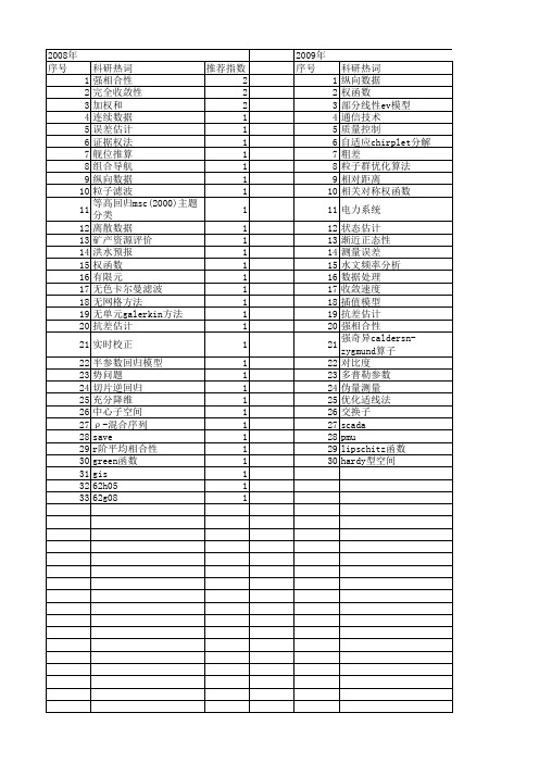
非参数估计方法张煜东;颜俊;王水花;吴乐南【摘要】为了解决函数估计问题,首先讨论了传统的参数回归方法.由于传统方法需要先验知识来决定参数模型,因此不稳健,且对模型敏感.因此,引入了基于数据驱动的非参数方法,无需任何先验知识即可对未知函数进行估计.本文主要介绍最新的8种非参数回归方法:核方法、局部多项式回归、正则化方法、正态均值模型、小波方法、超完备字典、前向神经网络、径向基函数网络.比较了不同的算法,给出算法之间的相关性与继承性.最后,将算法推广到高维情况,指出面临计算的维数诅咒与样本的维数诅咒两个问题.通过研究指出前者可以通过智能优化算法求解,而后者是问题固有的.【期刊名称】《武汉工程大学学报》【年(卷),期】2010(032)007【总页数】8页(P99-106)【关键词】参数统计;非参数统计;核方法;局部多项式回归;正则化方法;正态均值模型;小波;超完备字典;前向神经网络;径向基函数网络【作者】张煜东;颜俊;王水花;吴乐南【作者单位】东南大学信息科学与工程学院,江苏,南京,210096;哥仑比亚大学精神病学系脑成像实验室,纽约州,纽约,10032;东南大学信息科学与工程学院,江苏,南京,210096;东南大学信息科学与工程学院,江苏,南京,210096;东南大学信息科学与工程学院,江苏,南京,210096【正文语种】中文【中图分类】O212.70 引言函数估计[1]是一个经典反问题,一般定义为给定输入输出样本对,求未知的系统函数[2].传统的方法为参数方法,即构建一个参数模型,再定义某个误差项,通过最小化误差项来求解模型的参数[3].参数方法尽管较为简单,但不够灵活.例如参数模型假设有误,则会导致整个求解流程失败[4].因此学者们发展出不少新技术,非参数估计就是其中一项较好的方法.该方法无需提前假设参数模型的形式,而是基于数据结构推测回归曲面[5].本文首先研究了经典的2种参数回归方法:最小二乘法与内插函数法,分析了它们的不足,然后主要讨论8种非参数回归方法:核方法、局部多项式回归、正则化方法(样条估计)、正态均值模型、小波方法、过完全字典、前向神经网络、径向基函数网络,尤其详细介绍了其间的相关性与继承性.最后,研究了高维情况下面临的计算维数诅咒与样本维数诅咒.1 回归模型考虑模型yi=r(xi)+εi(1)式(1)中(xi,yi)为观测样本,假定误差ε具有方差齐性,则r=E(y|x)称为y对x的回归函数,简称回归.一般地,可以假设x取值在[0,1]区间内.定义“规则设计”为xi=i/n(i=1,2,…, n).并定义风险函数为(2)式(2)中为系统函数r的估计.回归一词源于高尔顿(Galton),他和学生皮尔逊(Pearson)在研究父母身高和子女身高的关系时,以每对夫妇的平均身高为x,取其一个成年儿子的身高为y,并用直线y=33.73+0.512x来描述y与x的关系.研究发现:如果双亲属于高个,则子女比他们还高的概率较小;反之,若双亲较矮,则子女以较大概率比双亲高.所以,个子偏高或偏矮的夫妇,其子女的身高有“向中心回归”的现象,因此高尔顿称描述子女与双亲身高关系的直线为“回归直线”[6].然而,并非所有的x-y函数均有回归性,但历史沿用了这个术语.更为精确的表达是“函数估计”.2 传统方法理论上描述一个函数需要无穷维数据,因此函数估计本身也可称为“无穷维估计”[7].传统的估计方法有下列两种极端情形.2.1 最小二乘法此时假设采用最小二乘法计算权值β=(β0,β1),得到的解为最小二乘估计[8],(3)则对给定样本点的估计可写为(4)这里Y=(y1,y2,…,yn)T.L=X(XTX)-1XT称为帽子矩阵[9].以5个样本点的一维规则设计矩阵为例,此时(5)L满足L=LT,L2=L.另外,L的迹等于输入数据的维数p,即trace(L)=p.这里输入数据是一维的,所以trace(L)=1.2.2 内插函数法此时对不加任何限制,得到的是该数据的一个内插函数[10].同样以5个样本点的一维规则设计矩阵为例,由于样本点的估计完全等于(y1,y2,…,yn)T,所以帽子矩阵为(6)2.3 两种方法的缺陷图1给出了这两种极端拟合的示意图,数据是被高斯噪声干扰的正弦函数,采用上述两种方法拟合,结果表明:最小二乘法过光滑,未展现数据内部的关系;而内插函数法忽略了噪声影响,显得欠光滑.从帽子矩阵也可看出,式(5)表明最小二乘法对每个数据的估计都利用了所有样本,这显然导致过光滑,且x值越大的数据权重越大,这明显与经验不符;反之,式(6)表明内插函数法仅仅利用了最邻近的样本数据,这显然导致欠光滑.图1 两种极端拟合Fig.1 Two extreme fitting2.4 非参数回归的优势非参数回归(non-parametric regression)作为最近兴起的一种函数估计方法,是一种分布无关(distribution free)的方法,即不依赖于数据的任何先验假设.与此对应的是参数回归(parametric regression),通常需要预先设置一个模型,然后求取该模型的参数.非参方法的本质在于:模型不是通过先验知识而是通过数据决定.需要注意的是,“非参数”并不表示没有参数,只是表示参数的数目、特征是可变的(flexible).由于非参方法无需数据先验知识,其应用范围较参数方法更广,且性能更稳健.其另一个优点是使用过程较参数方法更为简单.然而,它也存在缺点,一般结构更复杂,需要更多的运算时间.2.5 线性光滑器需要说明的是,最小二乘法、内插函数法、核方法、正则化方法、正态均值模型均是线性光滑器.定义为:若对每个x,存在向量l(x)=[l1(x),…,ln(x)]T,使得r(x)的估计可写为(7)则估计为一个线性光滑器[11].显然权重li(x)随着x而变化,这与信号处理中的“自适应滤波器”非常相似.3 核回归核方法[12]定义为(8)权重li由式(9)给出(9)这里h是带宽,K是一个核,满足K(x)≥0,以及(10)常用的核函数见表1.表1 常用的核公式Table 1 Frequently-used kernel formula核公式boxcarK(x)=0.5∗I(x)GaussianK(x)=12πexp-x22()EpanechnikovK(x)=34(1-x2)I(x)TricubeK(x)=7081(1-|x|3)3I(x)以boxcar核为例,帽子矩阵为(11)显然,这可视作最小二乘法与内插函数法的折中.为了估计带宽h,首先必须估计风险函数,一般可采用缺一交叉验证得分(12)这里为未用第i个数据所得到的估计,使CV最小的h,即为最佳带宽.为了加速运算,可将式(12)重新写为(13)这里Lii是光滑矩阵L的第i个对角线元素.另一种方法是采用广义交叉验证法,规定(14)这里v=tr(L).4 局部多项式回归采用核回归常会碰到下列2个问题[13]:1)若x不是规则设计的,则风险会增大,称为设计偏倚(design bias);2)核估计在接近边界处会出现较大偏差,称为边界偏倚(boundary bias).为了解决这2个问题,可采用局部多项式回归.局部多项式回归[14]可视作核估计的一个推广,首先定义权函数ωi(x)=K[(xi-x)/h],选择来使得下面的加权平方和最小(15)利用高等数学知识,可以看出解为(16)可见式(16)正好是核回归估计.这表明核估计是由局部加权最小二乘得到的局部常数估计.因此,若利用一个p阶的局部多项式而不是一个局部常数,就可能改进估计,使曲线更光滑.定义多项式(17)则局部多项式的思想是:选择使下列局部加权平方和(18)最小的a,估计依赖于目标值x,最终有(19)当p等于0时,等于核估计;当p=1时,称为局部线性回归(local linear regression)估计[15],由于其算法简单且性能优越,较为常用.5 基于正则化的回归为了描述方便,这里假设数据点为[(x0,y0),(x1,y1),…(xn-1,yn-1)].在风险函数(2)后增加一项惩罚项,一般设为r(x)的二阶导数(20)λ控制了解的光滑程度:当λ=0时,解为内插函数;当λ→∞时,解为最小二乘直线;当0<λ<∞时,是一个自然三次样条.需要注意下列事项:首先三次样条表示曲线在结点(knot)之间是三次多项式,且在结点处有连续的一阶和二阶导数;其次一个m阶样条为一个逐段m-1阶多项式,所以三次样条是4阶的(m=4);第三,自然样条表示在边界点处二阶导数为0,即在边界点外是线性的;第四,样条的结点等于数据点.为了加速计算,将数据点重新排序,假设a,b为样本点x的上下界,令a=t1≤t2≤…≤tn-1=b,这里t是x重新排序后的点,称为结点.可用B样条基(B-spline basis)[16]作为该三次样条的基,即(21)Pi称为控制点,共n-m个,形成一个凸壳.n-m个B样条基可通过如下计算,首先初始化:(22)然后对i=1,逐步+1,直到i=m-1,重复迭代下式:(23)若结点等距,则称B样条是均匀的(uniform),否则称为不均匀.如果两个结点相等,计算过程会出现0/0情况,此时默认结果为0.令矩阵B的第(i, j)元素bij=bj(xi),矩阵Ω的第(i, j)元素则控制点可由式(24)求得P=(BTB+λΩ)-1BTY(24)可见,样条也是一个线性光滑器.表面上看,基于核的估计与基于正则化的估计原理与模型均不一致,但是Silverman证明了如下定理,样条估计可视作如下所示的一种渐近的核估计(25)式中,f(x)是x的密度函数.(26)(27)显然,若样本x是规则设计,则f(x)=1, h(x)=(λ/n)1/4=h,li(x)∝K[(xi-x)/h],即此时样条估计可视作形如式(27)的渐近核估计.6 正态均值模型令φ1,φ2,…为一个标准正交基,则显然r(x)可以展开为定义(28)则随机变量Zj是正态分布,且均值与方差满足:E(Zj)=θj V(Zj)=σ2/n(29)可见,若估计出θ,则可近似求得因此正态均值模型将n个样本的函数估计问题转换为估计n个正态随机变量Zj的均值θ的问题[17].若直接令则显然得到一个很差的估计,下面给出风险更小的估计.首先,必须做出一个关于的风险估计,Stein给出下列定理:令为θ的一个估计,并令则的风险的一个无偏估计为(30)式中且D的第(i, j)个元素为g(z1,…,zn)的第i个元素关于zj的偏导数[18].假设式中b称为调节器,根据b的设置,存在下列3种情况:①b=(b,b,…,b),称为常数调节器(constant modulator),此时令式(30)最小的称为James-Stein估计;②b=(1,…,1,0,…,0),称为嵌套子集选择调节器(nested subset selection modulator),此时令式(30)最小的称为REACT方法.需要注意的是,若基选择傅立叶基,则该方法类似于频域低通滤波器方法.③b=(b1,b2,…,bn)满足1≥b1≥b2≥…≥bn≥0,称为单调调节器(monotone modulator),该方法理论最优,但是需要的运算量太大,几乎不实用.7 小波方法小波方法[19]适用于空间非齐次(spatially inhomogeneous)函数,即函数的光滑程度随着x会有本质性的变化.它可视作正态均值模型的推广,但存在两点区别:一是采用小波基代替传统的正交基,因为小波基较一般的正交基具有局部化的优点,能实现多分辨率分析;另一点是采用了一种称为“阈”的收缩方式.不妨假定父小波为φ,母小波为ψ,同时规定下标(j, k)的意义如下:fj,k(x)=2j/2f(2jx-k)(31)为了估计函数r,用n=2J项展开来近似r,(32)这里J0是任取常数,满足0≤J0≤J.α称为刻度系数,β称为细节系数.那么如何估计这些系数?首先计算(33)(34)Sk、Djk分别称为经验刻度系数与经验细节系数,可知Sk≈N(αj0,k,σ2/n),Djk≈N(βj,k,σ2/n),可估计方差为|∶k=0,…,2J-1-1)/0.6745(35)然后根据可得α与β的估计如下:(36)β的估计形式稍许复杂,采用硬阈与软阈的方式分别为(37)(38)之所以采用阈的形式,是因为稀疏性(sparse)的思想[20]:对某些复杂函数,在小波基上展开时系数也是稀疏的.因此,需要采用一种方式来捕获稀疏性.然而,传统的L2范数不能捕捉稀疏性,相反,L1范数与非零基数能够较好地捕捉稀疏性.例如,考虑n维向量a=(1,0,…,0)与b=(1/n1/2,…,1/n1/2),有‖a‖2=‖b‖2=1,可见,L2范数无法区分稀疏性.反之,‖a‖1=1,‖b‖1= n1/2,因此,L1范数能提取稀疏性;另外,若令非零基数为J(θ)={#(θi≠0)},则J(a)=1,J(b)=n,因此,非零基数也能提取稀疏性.最后,在正则化估计中若惩罚项分别为L1范数或非零基数,则最优估计恰好对应着软阈估计与硬阈估计.最后,需要解决阈估计中λ的计算问题,这里介绍两种最简单的方式:一是通用阈值(universal threshold),即对所有水平的分辨率阈值均一致,(39)另一种是分层阈值(level-by-level threshold),即对不同分辨率采用不同阈值,一般是通过最小化下式求得(40)式中nj=2j-1为在水平j的参数个数.8 超完备字典小波基较标准正交基的改进在于更加局部化,因此能实现对跳跃的捕捉.然而,虽然小波基非常复杂,但面对各种复杂的函数还是不够灵活.这种缺陷的根源在于:小波基是标准正交基,任意两个基函数之间正交,这保证了基函数简单完整的同时,也丧失了灵活性.基追踪(basis pursuit)方法[21]的思想是采用一种超完备(overcomplete)的基,例如对“光滑加跳跃”的函数,传统的傅立叶基能够捕捉光滑部分,但是难以捕捉跳跃部分;采用小波基能轻易捕捉跳跃部分,但是描述光滑部分较为困难.此时若将“傅立叶基”与“小波基”合并成一个新的基,则显然这种基能够轻松地估计“光滑加跳跃”函数.但是,这种新的基不再正交,它以牺牲正交性来获得更好的灵活性[22],故此时用“字典”来描述更精确,而本文为了简便统一仍采用“基”表述.9 前向神经网络以一个双层神经网络为例,记网络的输入神经元个数为m, 隐层神经元个数为n,输出层神经元个数为q,则网络结构如图2所示.图2 前向神经网络Fig.2 Forward neural network与上面几节线性方法不同的是,神经网络属于非线性统计数据建模(nonlinear statistical data modeling),其隐层暗含了“特征提取”的思想,且可视作输入数据在一种“自适应的非线性非正交的基”上的映射.同样地,此时基牺牲了正交性、线性、不变性,增加了计算负担,但换来了更加强大的灵活性[23].简而言之,前向神经网络采用了类似基追踪的方法[24],但基是自适应变化的、非线性的,因此更加灵活.前向神经网络与基追踪相似之处在于,两者的基都不是正交的,都是根据给定数据而自适应选取的最佳基.前向神经网络的优势在于无不需预选字典,字典在算法中自动生成,并可作为特征选择的一种方法.10 径向基函数网络首先观察径向基函数(RBF)神经元如图3所示.图3 RBF神经元图Fig.3 Neuron of RBF图中输入向量p的维数为R,首先p与输入层权值矩阵IW相减,然后求距离函数dist,再与偏置b1相乘,最后求径向基函数radbas(n)=exp(-n2),得到神经元的输出为a=radbas(‖IW-p‖b1)(41)整个RBF网络由两层神经元组成,第1层为S1个如图3所示的RBF神经元,第2层为S2个线性神经元,如图4所示.在第2层开始时,第1层的输出a首先经过线性层权值矩阵LW后与偏置b2相加,再通过一个纯线性(purelin)函数purelin(n)=n,得到网络输出y为y=purelin(LW×a+b2)(42)图4 RBF神经网络结构图Fig.4 Structure of RNN比较式(41)与式(9)可见,RBF网络与核方法非常类似,不同之处在于RBF网络的LW需要通过求解一个方程组,而核方法的权重是直接通过归一化计算求得,因此RBF网络预测结果更为逼近完全内插函数估计(注意不是未知函数r),而核方法计算更为简便[25].11 维数灾难将函数估计推广到高维,则会碰到维数诅咒(curse of dimensionality)[26](图5),它意味着当观测值的维数增加时,估计难度会迅速增大.维数诅咒有两层含义:一是计算的维数诅咒,指的是某些算法的计算量随着维数的增长而成指数增加.解决方法通常采用优化算法,例如遗传算法、粒子群算法、蚁群算法等[27].二是样本的维数诅咒,指的是数据维数为d时,样本量需要随着d指数增长.在函数估计中,第二层含义更为重要,这里给予详细解释.图5 样本的维数诅咒示意图Fig.5 Dimensionality curse of samples假设一个半径r维数为d的超球,被一个边长为2r维数为d的超立方体所包围,假设超立方体内存在一个均匀分布的点,则由于超球的体积为2rdπd/2/[dΓ(d/2)],超立方体的体积为(2r)d,因此该点同时也落在超球内的概率P为(43)令维数d由2逐步增长到20,则对应的概率P如图6所示.显然,当d=20时,P 仅为2.46×10⁻⁸.因此,若在2维空间中1个样本在半径r的意义下能逼近一个正方形,则在20维空间内,则需要1/2.46×10-8=4.06×107个样本才能在半径r的意义下逼近超立方体.图6 概率P与维数d的关系Fig.6 The curve of probability P against dimensionality d因此,在高维问题中,由于数据非常稀少,导致局部邻域中包含极少的数据点[28],因此估计变得异常困难.目前还没有较好的办法解决.12 结语将文中阐述的方法归结并示于图7.图7 非参数回归方法Fig.7 Survey of non-parametric regression methods不同类型方法的特点总结如下:a. 核方法、正则化方法、正态均值模型可以视作最基本最原始的方式.另外,正则化方法与正态均值模型可视作一类特殊的核方法.b. 核方法、局部多项式方法、正则化方法、正态均值模型、小波等方法在大多数情况下均非常类似.这些方法都包含了一个偏倚-方差平衡,所以都需要选择一个光滑参数.由于这些方法均是线性光滑器,所以均可以采用第4节中基于CV、GCV的方法.c. 小波方法一般面向空间非齐次函数.如果需要一个精确的函数估计,而且噪声水平较低,则小波方法非常有效.但若面对一个标准的非参数回归问题,而且感兴趣于置信集,则小波方法并不比其它方法明显更好.d. 超完备字典缺陷是丧失了基的正交性,因此估计系数变得复杂;优点是更为灵活,能够采用稀疏的系数描述复杂函数.e. 前向神经网络与RBF神经网络是基于不同的模型独立推导出来的,二者不可混淆.另外,神经网络方法的缺点是一般不考虑置信带,并常用训练误差代替风险函数,容易过拟合;优点是面向应用、思想简单且设计灵活.f. 理论上,这些方法没有大的差别,特别在用置信带的宽度来评价时.每种方法都有其拥护者与批评者,没有哪一种方法目前获得应用上的优势.一种解决方案是对每个问题都利用所有可行的方法,如果结果一致,则选择简单者;如果结果不一致,则必须探讨内在的原因.g. 所讨论的方法能够用于高维问题,然而,即使通过智能优化算法解决了计算的维数诅咒,仍然面对样本的维数诅咒.计算一个高维估计相对容易,然而该估计将不如一维情况下那么精确,其置信区间会非常大.但这并不表示方法失效,而是表示问题的固有困难.参考文献:[1]Neumeyer N.A note on uniform consistency of monotone function estimators [J]. Statistics & Probability Letters,2007,77(7):693-703[2]Sheena Y,Gupta A K.New estimator for functions of the canonical correlation coefficients [J]. Journal of Statistical Planning and Inference,2005,131(1):41-61.[3]张煜东,吴乐南,李铜川,等.基于PCNN的彩色图像直方图均衡化增强[J].东南大学学报,2010,40(1):64-68.[4]詹锦华.基于优化灰色模型的农村居民消费结构预测[J].武汉工程大学学报,2009,31(9):89-91.[5]Wasserman L. All of Nonparametric Statistics [M].New York:Springer-Verlag, Inc.[6]张煜东, 吴乐南, 吴含前.工程优化问题中神经网络与进化算法的比较[J].计算机工程与应用,2009,45(3):1-6.[7]Hansen C B.Asymptotic properties of a robust variance matrix estimator for panel data when T is large [J].Journal of Econometrics,2007,141(2):597-620.[8]Pokharel P P, Liu W F, Principe J C.Kernel least mean square algorithm with constrained growth [J].Signal Processing,2009,89(3):257-265.[9]Kalivas J H.Cyclic subspace regression with analysis of the hat matrix [J].Chemometrics and Intelligent Laboratory Systems,1999,45(1):215-224.[10]张煜东,吴乐南.基于二维Tsallis熵的改进PCNN图像分割[J].东南大学学报:自然科学版,2008,38(4):579-584[11]Geçkinli N C, Yavuz D.A set of optimal discrete linearsmoothers[J].Signal Processing,2001,3(1):49-62.[12]Antoniotti M,Carreras M,Farinaccio A,et al.An application of kernel methods to gene cluster temporal meta-analysis [J].Computers & Operations Research,2010,37(8):1361-1368.[13]Hsieh P F,Chou P W,Chuang H Y.An MRF-based kernel method for nonlinear feature extraction [J].Image and VisionComputing,2010,28(3):502-517.[14]Katkovnik V.Multiresolution local polynomial regression:A new approach to pointwise spatial adaptation [J].Digital Signal Processing,2005,15(1):73-116.[15]Baíllo A,Grané A.Local linear regression for functional predictor and scalar response [J].Journal of Multivariate Analysis,2009,100(1):102-111.[16]Zhang J W,Krause F L.Extending cubic uniform B-splines by unified trigonometric and hyperbolic basis [J].Graphical Models,2005,67(2):100-119.[17]张煜东,吴乐南,韦耿,等.用于多指数拟合的一种混沌免疫粒子群优化[J].东南大学学报,2009,39(4):678-683.[18]Chaudhuri S,Perlman M D.Consistent estimation of the minimum normal mean under the tree-order restriction [J].Journal of Statistical Planning and Inference,2007,137(11):3317-3335.[19]Labat D.Recent advances in wavelet analyses:Part 1.A review of concepts[J].Journal of Hydrology,2005,314(1):275-288.[20]Kunoth A.Adaptive Wavelets for Sparse Representations of Scattered Data[J].Studies in Computational Mathematics,2006,12:85-108.[21]Donoho D L, Elad M.On the stability of the basis pursuit in the presence of noise[J].Signal Processing,2006,86(3):511-532.[22]Malgouyres F.Rank related properties for Basis Pursuit and total variation regularization [J].Signal Processing,2007,87(11):2695-2707. [23]张煜东,吴乐南,韦耿.神经网络泛化增强技术研究[J].科学技术与工程,2009,9(17):4997-5002.[24]屠艳平,管昌生,谭浩.基于BP网络的钢筋混凝土结构时变可靠度[J].武汉工程大学学报,2008,30(3):36-39.[25]Zhang Y D,Wu L N,Neggaz N, et al.Remote-sensing Image Classification Based on an Improved Probabilistic NeuralNetwork[J].Sensors,2009,9:7516-7539.[26]Aleksandrowicz G,Barequet G.Counting polycubes without the dimensionality curse [J].Discrete Mathematics,2009,309(13):4576-4583. [27]张煜东,吴乐南,奚吉,等.进化计算研究现状(上)[J].电脑开发与应用,2009,22(12):1-5.[28]王忠,叶雄飞.遗传算法在数字水印技术中的应用[J].武汉工程大学学报,2008,30(1):95-97.。
I.J. Information Engineering and Electronic Business, 2011, 1, 9-15Published Online February 2011 in MECS (/)Irregular Function Estimation with LR-MKRWeiwei HanDepartment of Mathematics & Computer Science of Guangdong University of Business Studies, Guangzhou, ChinaEmail: hww_2006@Abstract —Estimating the irregular function with multi-scale structure is a hard problem. The results achieved by thetraditional kernel learning are often unsatisfactory, sinceunderfitting and overfitting cannot be simultaneouslyavoided, and the performance relative to boundary is oftenunsatisfactory. In this paper, we investigate the data-based local reweighted regression model under kernel trick and propose an iterative method to solve the kernel regression problem, local reweighted multiple kernel regression (LR-MKR). The new framework of kernel learning approach includes two parts. First, an improved Nadaraya-Watson estimator based on blockwised approach is constructed to organize a data-driven localized reweighted criteria; Second, an iterative kernel learning method is introduced in a series decreased active set. Experiments on simulated and real data sets demonstrate the proposed method can avoid under fitting and over fitting simultaneously and improve the performance relative to the boundary effetely.Index Terms —irregular function, statistic learning, multiple kernel learningI. I NTRODUCTIONLearning to fit irregular data with noise is an important research problem in many real-world data mining applications, which can be viewed as a function approximation from sample data. Kernel tricks have attracted more and more research attention recently. For kernel methods, the data representation should be implicitly chosen through the kernel function. Because this kernel actually plays several roles: it defines the similarity between two examples x and x ′, while defining an appropriate regularization term for learning problem. Choosing a kernel K is equivalent to specifying a prior information on a Reproducing Kernel Hilbert Space (RKHS), therefore having a large choice of RKHS should be fruitful for the approximation accuracy, if over fitting is properly controlled, since one can dapt its hypothesis space to each specific data set [1]-[3] For given data set 1{(,)}n i i i S x y ==. Assume that()m x H ∈, where H is some reproducing kernelHilbert space called active space, with respect to the reproducing kernel K . The square norm related to the inner productby 2||||,HHf f f =. Consider theproblem,1min ()(,())()n i i i H m L y m x P m λ==+∑Where λ is a positive number which balances the trade-off between fitness and smoothness; L is a loss function which determines how different between i y and ()i m x and should be penalized; ()P m is a function which denotes the prior information on the function ()m ⋅. When the penalized function ()P ⋅ is defined as2()||||H p m m =. By the represent theory, the solution ofthe upper kernel learning problem is of the general form1()(,)niii m x K x x α==∑ (1)Where i α are the coefficients to be learned from the examples, while K is positive definite kernel associated with RKHS H . It should be noted that m can also be expressed with regards to the basis elements of H as()()i i m x x αφ=∑, which is called the dual from of m . An advantage of using the kernel representationgiven in (1) is that the number of coefficients to be estimated depends only on n and not on cardinality of the basis, which may be infinite. It is this properly that makes the kernel methods so popular, see, e.g. [16]. Recently, using multiple kernels instead of a single one can enhance the interpretability and improve performance [1]. In such cases, a convenient approach is to consider: 11(,)(,),..1,0N Niiii i i K x x c K x x s t c c ==′′==≥∑∑ (2)Where N is the total number of kernels. Interpretabilitycan then be enhanced by a careful choice of the kernels, j K and their weighting coefficients, i c . Each basis kernel j K may either use the full set of variables describing x or only a subset of these variables. Within this framework, the multiple kernel learning problem is transformed to learning both the coefficients i αand the weights jc in a single optimization problem.Unfortunately, it is difficult problem to search the optimal parameters in 2-dimention space in irregular function regression problem. In addition, it ignored that a sequence of kernels will induce representation redundancy inevitably and will increase computational burden as a result of much more parameters. Also, the correct number of kernels N is unknown, and simultaneously determining the required number of10 Irregular Function Estimation with LR-MKRkernels as well as estimating the associated parameters of MKL is a challenging problem [1].For irregular functions which comprise both the steep variations and the smooth variations, it is sometimes unsuitable to use one kernel even if a composite multiple kernel with several global bandwidths to estimate the unknown function [2]. First, the kernels are chosen prior to learning, which may be not adaptive to the characteristics of the function so that under fittings and over fittings occur frequently in the estimated function [3]. Although, the localized multiple kernel learning proposed in [4] is adaptive to portions of high and low curvature, it is sensitive to initial parameters. Second, how to determine the number of kernels is unanswered. Finally, classical kernel regression methods exhibit a poor boundary performance [5][6][7]. In order to estimate an irregular function, this paper proposed an improved Nadaraya-Watson estimator approach to produce localized data-driven reweighted multiple kernel learning method; Different from classical MKL, we solve the MKL problem in a series decreased active subspace. Simulations show that the performance of the proposed method is systematically better than a fixed RBF kernel. The rest of this correspondence is organized as follows. In section 2, we proposed an iterative localized regression to deal with non-flat function regression problem. Section 3 presented regression results on numerical experiments on synthesis and real-world data sets while section 4 concludes the paper and contains remarks and other issues about future work.II. T HE LOCALIZED REWEIGHTED MULTIPLE KERNELREGRESSION METHOD In order to achieve the objects refer to abstract, we suggest adherence to the following recommendations. Different from the simple combination of several basis kernels, we proceed a new multiple kernel learning on a sequence of nested subspaces based on iteration approach. During iteration, the active subspace is decreasing while the classical multiple kernel regression is not.A. The Improved Nadaraya-Watson EstimatorNadaraya(1964) [8] and Watson(1964) [9] proposed to estimate ()m x using a kernel as a weighting function. Given the sample data set 1{(,)}n i i i S x y ==:111(,)ˆ(;)(;)(,)nnh i ii i i ni hi i K x x y mx S w x S y K x x =====∑∑∑Where 11(;)[(,)](,)ni hi h i i w x S Kx x K x x −==∑ is theNadaraya-Watson weights, such that1(;)1,njj w x S x ==∀∑And1()(/)h K x h K x h −= is a kernel withbandwidth h .Associating blockwise technique, we propose an improved localized kernel regression estimator which achieves automatic data-driven bandwidth selection [10]. Suppose the initial data set S is partitioned into p blocks denote by 12,,...,p SS SS SS with length12,,...,p d d d such that 1pj j b n ==∑[11]. For given x , ifthere is some block x SS such thatmin{|}max{|}i i x i i x x x SS x x x SS ∈≤≤∈Then the block wised Nadaraya-Watson estimator is given as follows(,)ˆ(;)(;)(,)i xi xi xh i i x SS xi x ix SS h i x SS K x x y mx SS w x SS y K x x ∈∈∈==∑∑∑As thus, the localized estimator presents the unknown function m without a complicated parameters selection procedure.B. The new regression methodGiven a dataset,{(,),,}ni i i i S x y x R y R =∈∈. Assume that ()m x H ∈, where H is some reproducing kernel Hilbert space called active space, with respect to the reproducing kernel K . The square norm related to the inner productby 2,HHf f f=. Consider theproblem,1min ()(,())()ni i i H m L y m x P m λ==+∑ (3)Where λ is a positive number which balances the trade-off between fitness and smoothness; L is a loss function;2()HP m m= is penalized function. By the representtheory, the solution of equation (3) is [12],1ˆ()(,)ni i i mx K x x α==∑ (4) A generalized framework of kernel is defined as1(,)(,)Ni i i K x x c K x x =′′=∑ (5)Where ,1,...,i K i N = are N positive definite kernels on the same input space X , and each of them beingassociated to a RKHS i H whose elements will be denoted i f and endowed with an inner product ,i ⋅, and 1{}Ni i c = are coefficients to be learned under the nonnegative and unity constraints11,0,1Nii i cc i N ==>≤≤∑ (6)How to determine N is an unanswered problem. For any 0i c >, i H ′ is the Hilbert space derived from i H as follows:{|:}iH i i if H f f H c ′=∈<∞Endowed with the inner product1,,i H i if gf g c ′=Within this framework, i H ′ is a RKHS with kernel (,)i i i K c K x x ′′=, since()(),(,)(),(,)ii i i i H H m x m K x m c K x ′=⋅⋅=⋅⋅Then, we define H as the direct sum of the RKHS i H ′. Substituting (5) into (4), an updated equation of (2) is obtained as follows,111111ˆ()(,)(,)(,)()ni i i nNi j j i i j Nnj i j i j i Nj j mx K x x c K x x c K x x m x ααα==========∑∑∑∑∑∑ (7)Instead of the equation (3), we convert to consider themodels for 1,...,j N =,1min ()(,())()nj j i j i j j i H m L y m x P m λ==+∑ (8)Then, the kernel learning problem can thus be envisioned as learning a predictor belonging to a series of adaptive hypothesis space endowed with a kernel function. The forthcoming part explains how we solve this problem. Assume that a kernel function 1(,)K ⋅⋅ and corresponding reproducing kernel Hilbert space 1H ′ are included, and then we get the initial estimator,111(,)ˆ()(,)i ji jph i i j x SS ph i j x SS K x x y mx K x x =∈=∈=∑∑∑∑(9)The residual function can be obtained,1111ˆ()()()res x m x mx V H H ′=−∈=− (10) If we have introduced t kernels 1{}tj j K =, then the estimator can be updated as111ˆˆ()()(,)t t nj j i j i j j i mx m x K x x α=====∑∑∑ And the residual function,ˆ()()()t res x m x mx =− (11) If the measurements of t res fulfilled certain thresholding criteria, here we employ 2-norm, N t = represents thenumber of introduced kernels and puts an end toiteration procedure. If not, considering the problem in the decreased subspace 1t H +′, computeˆ()i i i res y mx =− and update the sample set {(,)}i i S x res = which can be treated as the limited of the initial data set in 1t H +′. Employing iteration, we willconsider a new regression problem on the updated sample data set in a decreased subspace.Compared with the general multiple kernel learning (MKL), the first advantage is that it needs not to select weights i α which will reduce much more computation burden and just need to select one kernel bandwidth at each iteration step. Furthermore, the new method is adaptive to the local curvature variation and improves the boundary performance as a result of the introduction of blockwised Nadaraya-Watson estimate technique. At last, the number of kernels introduced will change according to real data settings based on iteration which will avoid under fitting and over fitting problem effectively. C .LR-MKR AlgorithmThe complete algorithm of Iterative Localized Multiple Kernel Reweighted Regression can be briefly described by the following steps:1) Input S , the maximum iterarion step M , the threshold ε, and 1N =;2) Initialize the pilot estimator ˆ()0mx =, and pilot residual e y =;3) Update the data set 1{(,)}nj j j S x e ==;4) Select kernel K , compute the estimator ˆ(;)mx S with equation (9); 5) Update the estimator ˆ()()(;)m x m x mx S =+; 6) Update the residuals ()e y m x =−, and update 1N N =+;7) Calculate the norm of residual e .Repeating the steps from 3) to 7), this process is continued until the norm of residual e is smaller than the pre-determined value ε or the number of iteration step N is larger than the pre-determined value M .The algorithm of Localized Reweighted Multiple Kernel Regression algorithm is adaptive to different portions with different curvatures and is not sensitive to noise level and the pilot estimation. One kernel in one interation step the new method avoids the representation redundance problem effectively. Although the choice of optimal kernel and associated parameters have been investigated by many model selection problems, the model parameters are generally domain-specific. The Gaussian kernel is most popularly used when there is no prior knowledge regarding the data.In order to select parameters, we choose 10-fold cross-validation: randomly divide the given data into ten blocksand consider the Generalized Cross Validation function is given as()21ˆ()()10j jGCV m m θ−=−∑ Where θ represents the set of relevant parameters, and()ˆj m− is the estimator of m without the jth block samples of S . Smaller values of the GCV function implybetter prediction performance. Thus, among a possible set of parameters, the optimal value is the minimized of the GCV function.Ⅲ. EXPERIMENT RESULTSWe have conducted studies on simulated data and real-world data using the proposed method. Each experiment is repeated 50 times with different random splits in order to estimate the numerical performance values. Some of the results are reported in the following. We decide to use, as it is done often, Gaussian radial basis kernel which not only satisfies Mercer’s conditions for kernels, but also is most widely used. Mercer’s conditions are illustrated in Scholkopf (2002) [3]. In classical MKL, it rises not only how many kernels to chose but also which one to choose. A. Application to Simulated Data (1) At first, we consider the test function2()5sin(2)exp(16/50)m x x x =−To examine the performance of regression algorithm. In this experiment, three random samples of size 100, 200, 500 were generated uniformly from the interval [-5,5], respectively. The target values are then corrupted by some noise with a normal distribution 2(0,)N σ. The standard deviation σ is 0.4 and 1, which determines the noise level.Which has different curvature for different design, so a global bandwidth can not deal with well. It is well known that around the peak of the true regression function ()m x the bias of the estimate is particularly important. So, in such areas, it would be better to choose a small bandwidth to reduce these bias effects. Conversely, a larger bandwidth could be used to reduce variance effects, without letting the bias increase too much, when the curve is relatively flat [14]. Experiments result shows that the new method could deal this intrinsic shortcoming well combining with the improved Nadaraya-Watson estimation and iteration approach.Figure 1 presents the curves of the test function (slender line) and the estimation curves (bold line) when the additive Gaussion noise is (0,1)N . Figure 1(a) demonstrates the test function and sample data; Figure 1(b) shows the estimated curve using the proposed method with two step iteration which deals well with different portions with different curvature; Figure 1(c) demonstrates the standard single kernel regression based on Gaussian kernel with a global bandwidth which was determined through GCV. The mean-square error (MSE) is adopted as the performance metric, which has beenwidely used in regression tasks. In the experiment, we generated several versions of data sets with different noise level. Then, we repeated each experiment up to 50 runs and summarized average results in Table 1. From the experimental results, several observations can be drawn. First, compared with single kernel regression, the iterative localized reweighted multiple kernel regression could adapt to different portions with different curvature and it could avoid under fitting and over fitting simultaneously. Second, the proposed method shows a better boundary performance. At last, the numerical results show that the new method is less sensitive to the noise level when the sample size is fixed.(a)(b)(c)Figure 1. Demonstration of LR-MKL results: the test function (slender line) and the approximation function (bold line). Figure (a) demonstrates the test function and noised sample data; Figure (b) shows the estimated curve using the proposed method which deals with well with different portion of different curvature; Figure (c) demonstrates the standard single kernel regression results(1σ=).TABLE I.THE AVERAGED EXPERIMENTAL RESULTS OVER 50REPETITIONS FOR EACH SITUATION . AND THE MSE IS ADOPTED AS THEMETRICn1002005000.4σ= 0.0226 0.0152 0.0074 1σ=0.02580.01570.0076(a)(b)(c)Figure 2. The test function (slender line) and the approximation function (bold line). Figure (a) shows simulated data with white noise (SNR=20); Figure (b) shows the estimated curve using the new method; Figure (c) demonstrates the standard single kernel regression result.B. Application to Simulated Data (2)The test function is the mixture of Gaussian and Laplacian distributions define by2(2)0.7220.7()4x x m x e−−−+=+The number of data points for experiment is 200, and the experiment was repeated 50 times. Figure 2(a) shows the target values which were corrupted by white noise. The performance of the experiment was shown in Figure 2, in which the slender line present the true test function and the bold line represented the estimated results. Figure 2(b) represented the estimated curve using the proposed method with two step iteration which deals well with different portions with different curvature; Figure 2(c) demonstrated the standard single kernel regression based on Gaussian kernel with a global bandwidth. For this example, it can be seen that the Iterative Localized Multiple Kernel regression method achieved the better performance. Compared with the proposed method, the single kernel regression could not avoid under fitting and over fitting simultaneously and sensitive to the noise at boundary area.C. Application to real data: Burning Ethanol DataIn order to evaluate the performance of our proposed method in practice, we analyzed the Burning Ethanol Data set. Figure 3(a) shows the data set of Brinkmann (1981) that has been analyzed extensively. The data consist of 88 a measurement from an experiment in which ethanol was burned in a single cylinder automobile test engine. Because of the nature of the experiment, the observations are not available at equally-spaced design points, and the variability is larger for low equivalence ratio.As we all know, it is a difficult problem to control the pump around 0.8. Figure 3 shows the Iterative Localized Multiple Kernel regression results with different parameters and iteration steps. The red line represents the single kernel estimator. The blue in figure 3(b)-(c) represent the estimators after two and three steps iteration with different kernel bandwidths which are determined by GCV. From the experimental results, several advantages can be drawn. First, all the estimated curves have not a spurious high-frequency feature when the equivalence ratio is around 0.8 which is the drawback other regression methods must deal with cautiously. Second, compared with [13], the proposed method is not sensitive to the pilot estimator and the kernel bandwidth selection. Finally, all the fitting results show the good boundary performance.D. CUP TimeAll the experiments were implemented in the environment of MATLAB-7.0 on 2.6 GHz Pentium 4 machine with 2-G RAM. Table 2 presents the average CPU time (second) of the general single kernel regression (SK) and the proposed method (LR-MKR) on simulation 1 for three training sample sizes 100, 200, 500, each sample size has been run 50 times. It can be seen that the proposed method needs more CPU time than the general single kernel regression as a result of multiple kernels to be introduced.(a)(b)(c)Figure 3. Figure (a) shows Burning Ethanol Data; The blue bold lines in figure (b) and (c) show different estimated curves with two and three kernels.TABLE II. TRAINING TIMES (SECONDS) OF GENERAL SINGLEKERNEL REGRESSION (SK) AND THE NEW METHOD (LR-MKR) ONSIMULATION 1.Samplesize100 200100 0.3120 0.3276200 0.3588 0.9204500 2.7456 5.5068Ⅳ.CONCLUSIONS AND DISCUSSIONIn this paper, we consider the kernel trick and proposed an iterative localized reweighted multiple kernel regression method which includes two parts. At first, an improved Nadaraya-Watson estimator is introduced based on blockwised approach to produce an localized data-driven reweighting method, which improves the classical Nadaraya-Watson estimator to be adaptive to different portions with different curvatures; Then, considering the shortcoming of general multiple kernel regression, we convert to iteration in a series decreased active subspaces and proposed a novel kernel selection framework during iteration procedure which simultaneously avoids under fitting and over fitting effectively. The presentation covers the curves both deep variation and smooth variation. The simulation results show that the proposed method is less sensitive to noise level and pilot selection. Furthermore, experiments on simulated and real data set demonstrate that the new method is adaptive to the local curvature variation and could improve boundary performance effectively. It is easy to extend the method to other type additive noise. Kernel function plays an important role in kernel trick and can only work well in some circumstances, so, how to construct a new kernel function according to the given sample data settings is another direction we will keep up with.R EFERENCES[1]G. R. G. Lanckriet, T. D. Bie, N. Cristianini, M. I. Jordanand W. S. Noble, “A statistical framework for genomic data fusion,” Bioinformatics, vol.20, pp. 2626-2635, 2004.[2] D. Zheng, J. Wang and Y. Zhao, “Non-flat functionestimation with a muli-scale support vector regression,”Neurocomputing, vol. 70, pp. 420-429, 2006.[3] B. Scholkopf and A. J. Smola, Learning with Kernels.London, England: The MIT Press, Cambbrige, Massachusetts, 2002.[4]M. Gonen and E. Alpaydin, “Localized multiple kernellearning,” in Processing of 25th International Conference on Machine Learning, 2008.[5]M. Szafranski, Y. Grandvalet and A. Rakotomamonjy,“Composite kernel learning,” in P rocessing of the 25th International Conference on Machine Learning, 2008. [6]G. R. G. Lanckriet, “Learning the kernel matrix withsemidefinite programming,” Journal of Machine Learning Research, vol. 5, pp. 27-72, 2004.[7] A. Rakotomamonjy, F. Bach, S. Canu and Y. Grandvale,“More efficiency in multiple kernel learning,” Preceedings of the 24th international conference on Machine Learning, vol. 227, pp. 775-782, 2007.[8] E. A. Nadaraya, “On estimating regression,” Theory ofprobability and Its Applications, vol. 9, no. 1, pp. 141-142, 1964.[9]G. S. Watson, “Smooth regression analysis,” Sankhya, Ser.A, vol. 26, pp. 359-372, 1964.[10]Y. Kim, J. Kim and Y. Kim, “Blockwise sparseregression,” Statistica Sinica, vol. 16, pp. 375-390, 2006. [11]L. Lin, Y. Fan and L. Tan, “Blockwise bootstrap waveletin nonparametric regression model with weakly dependent processes,” Metrika, vol. 67, pp. 31-48, 2008.[12]A. Tikhonov and V. Arsenin, Solutions of Ill-posedProblem, Washingon: W. H. Winston, 1977.[13]A. Rakotomamonjy, X, Mary and S. Canu, “Non-parametric regression with wavelet kernels,” Applied Stochastic Models in Business and Industry, vol. 21, pp.153-163, 2005.[14]P. Vieu, “Nonparametric regression: Optimal localbandwidth choice,” Journal of the Royal Statistical Society.Serie B (Methodological), vol.53, no. 2, pp. 453-464, 1991.[15]X. M. A. Rakotomamonjy and S. Canu, “non-parametricregression with wavelet kernels,” Applied Stochastic Models in Business and Industry, vol. 21, pp. 153-163, 2005.[16]W. F. Zhang, D. Q. Dai and H. Yan, “Framelet kernelswith applications to support vector regression and regularization networks,” IEEE Transactions on System, Man and Cybernetics, Part B, vol. 40, pp. 1128-1144, 2009.Weiwei Han received the M.S. degree inmathematics from Zhongshan University,Guangzhou, China, in 2005.She is a teaching staff in GuangdongUniversity of Business Study. Her researchinterests include statistical learning,machine learning and data mining.。