基于核函数的学习算法经典.ppt
- 格式:ppt
- 大小:1.36 MB
- 文档页数:38


基于核函数的学习算法基于核函数的学习算法是一种机器学习算法,用于解决非线性分类和回归问题。
在传统的机器学习算法中,我们通常假设样本数据是线性可分或线性可回归的,但是在现实世界中,许多问题是非线性的。
为了解决这些非线性问题,我们可以使用核函数来将原始数据映射到高维特征空间中,然后在该特征空间中进行线性分类或回归。
核函数是一个用于计算两个向量之间相似度的函数。
它可以通过计算两个向量在特征空间中的内积来度量它们的相似程度。
常用的核函数包括线性核函数、多项式核函数、高斯核函数等。
支持向量机是一种非常有力的分类算法。
它利用核技巧将输入数据映射到高维特征空间中,然后在该特征空间中找到一个最优分割超平面,使得样本点离超平面的距离最大化。
通过最大化间隔,支持向量机能够更好地处理非线性分类问题,并具有较好的泛化性能。
支持向量机的核函数可以将样本数据映射到高维特征空间中,以便在非线性问题上进行线性分类。
常用的核函数包括线性核函数、多项式核函数和高斯核函数等。
线性核函数可以实现与传统线性分类算法相同的效果。
多项式核函数可以将数据映射到多项式特征空间中,通过多项式特征的组合实现非线性分类。
高斯核函数可以将数据映射到无穷维的特征空间中,通过高斯核函数的相似度计算实现非线性分类。
核岭回归是一种非线性回归算法。
类似于支持向量机,核岭回归也利用核函数将输入数据映射到高维特征空间中,然后在该特征空间中进行线性回归。
通过最小二乘法求解岭回归问题,核岭回归能够更好地处理非线性回归问题。
1.能够处理非线性问题:核函数能够将数据映射到高维特征空间中,从而实现对非线性问题的线性分类或回归。
2.较好的泛化性能:支持向量机等基于核函数的学习算法通过最大化间隔来进行分类,可以有较好的泛化性能,减少模型的过拟合风险。
3.算法简洁高效:基于核函数的学习算法通常具有简单的模型结构和高效的求解方法,能够处理大规模数据集。
4.不依赖数据分布:基于核函数的学习算法不依赖于数据的分布情况,适用于各种类型的数据。
高斯核函数:深度学习中的经典工具
在深度学习领域中,高斯核函数一直是一个备受关注的经典工具。
它不仅可以有效地解决回归和分类等任务,还可以应用于图像和语音
识别等领域。
那么,高斯核函数是如何计算的呢?本文将介绍高斯核
函数的计算方法及其应用。
首先,高斯核函数是一种基于距离的相似度度量方式。
它可以将
样本空间中的点映射到高维空间中,使得原本线性不可分的数据变成
线性可分的数据。
具体而言,我们可以用以下公式来表示高斯核函数:K(x_i, x_j) = exp(-|| x_i - x_j ||^2 / (2 * sigma^2))
其中,x_i和x_j分别表示样本空间中的两个点,sigma为高斯核
函数的参数,|| x_i - x_j ||^2为欧氏距离的平方。
在实际计算过程中,高斯核函数通常与支持向量机(SVM)算法结
合使用,来进行分类和回归等任务。
在SVM算法中,高斯核函数可以
将原始数据映射到一个高维空间中,并计算多维空间中数据的内积,
从而得出分类结果。
具体而言,高斯核函数可以通过SVM的拉格朗日
乘子来计算。
除此之外,高斯核函数还可以应用于图像和语音识别等领域。
例如,在图像识别中,可以通过高斯核函数来进行图像特征提取,从而
实现图像分类和识别。
在语音识别中,可以通过高斯核函数来进行声
学模型训练,从而实现语音识别的精准度提升。
综上所述,高斯核函数作为深度学习中的经典工具,不仅能够有效地解决回归和分类等问题,还可以应用于图像和语音识别等领域。
因此,如果你想要开展深度学习相关的研究,那么请不要错过这个重要的工具!。

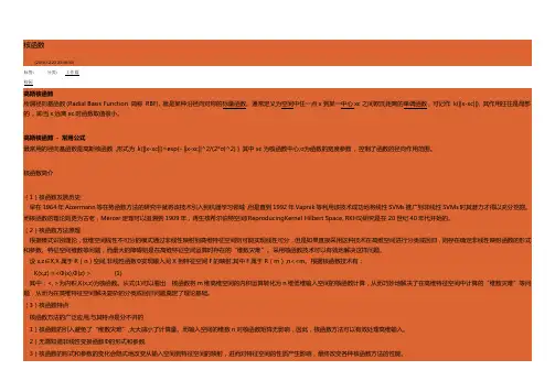
核函数(2010-12-23 23:08:30)分类:工作篇标签:校园高斯核函数所谓径向基函数(Radial Basis Function 简称 RBF), 就是某种沿径向对称的标量函数。
通常定义为空间中任一点x到某一中心xc之间欧氏距离的单调函数, 可记作 k(||x-xc||), 其作用往往是局部的 , 即当x远离xc时函数取值很小。
高斯核函数 - 常用公式最常用的径向基函数是高斯核函数 ,形式为 k(||x-xc||)=exp{- ||x-xc||^2/(2*σ)^2) } 其中xc为核函数中心,σ为函数的宽度参数 , 控制了函数的径向作用范围。
核函数简介(1)核函数发展历史早在1964年Aizermann等在势函数方法的研究中就将该技术引入到机器学习领域,但是直到1992年Vapnik等利用该技术成功地将线性SVMs推广到非线性SVMs时其潜力才得以充分挖掘。
而核函数的理论则更为古老,Mercer定理可以追溯到1909年,再生核希尔伯特空间(ReproducingKernel Hilbert Space, RKHS)研究是在20世纪40年代开始的。
(2)核函数方法原理根据模式识别理论,低维空间线性不可分的模式通过非线性映射到高维特征空间则可能实现线性可分,但是如果直接采用这种技术在高维空间进行分类或回归,则存在确定非线性映射函数的形式和参数、特征空间维数等问题,而最大的障碍则是在高维特征空间运算时存在的“维数灾难”。
采用核函数技术可以有效地解决这样问题。
设x,z∈X,X属于R(n)空间,非线性函数Φ实现输入间X到特征空间F的映射,其中F属于R(m),n<<m。
根据核函数技术有:K(x,z) =<Φ(x),Φ(z) >(1)其中:<, >为内积,K(x,z)为核函数。
从式(1)可以看出,核函数将m维高维空间的内积运算转化为n维低维输入空间的核函数计算,从而巧妙地解决了在高维特征空间中计算的“维数灾难”等问题,从而为在高维特征空间解决复杂的分类或回归问题奠定了理论基础。
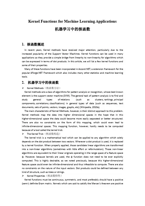
Kernel Functions for Machine Learning Applications机器学习中的核函数1.核函数概述In recent years, Kernel methods have received major attention, particularly due to the increased popularity of the Support Vector Machines. Kernel functions can be used in many applications as they provide a simple bridge from linearity to non-linearity for algorithms which can be expressed in terms of dot products. In this article, we will list a few kernel functions and some of their properties.Many of these functions have been incorporated in , a extension framework for the popular Framework which also includes many other statistics and machine learning tools.2.机器学习中的核函数Kernel Methods(核函数方法)Kernel methods are a class of algorithms for pattern analysis or recognition, whose best known element is the support vector machine (SVM). The general task of pattern analysis is to find and study general types of relations (such as clusters, rankings, principal components, correlations, classifications) in general types of data (such as sequences, text documents, sets of points, vectors, images, graphs, etc) (Wikipedia, 2010a).The main characteristic of Kernel Methods, however, is their distinct approach to this problem. Kernel methods map the data into higher dimensional spaces in the hope that in this higher-dimensional space the data could become more easily separated or better structured. There are also no constraints on the form of this mapping, which could even lead to infinite-dimensional spaces. This mapping function, however, hardly needs to be computed because of a tool called the kernel trick.The Kernel Trick(核函数构造)The kernel trick is a mathematical tool which can be applied to any algorithm which solely depends on the dot product between two vectors. Wherever a dot product is used, it is replaced by a kernel function. When properly applied, those candidate linear algorithms are transformed into a non-linear algorithms (sometimes with little effort or reformulation). Those non-linear algorithms are equivalent to their linear originals operating in the range space of a feature space φ. However, because kernels are used, the φ function does not need to be ever explicitly computed. This is highly desirable, as we noted previously, because this higher-dimensional feature space could even be infinite-dimensional and thus infeasible to compute. There are also no constraints on the nature of the input vectors. Dot products could be defined between any kind of structure, such as trees or strings.Kernel Properties(核函数特性)Kernel functions must be continuous, symmetric, and most preferably should have a positive (semi-) definite Gram matrix. Kernels which are said to satisfy the Mercer's theorem are positivesemi-definite, meaning their kernel matrices have no non-negative Eigen values. The use of a positive definite kernel insures that the optimization problem will be convex and solution will be unique.However, many kernel functions which aren’t strictly positive definite also have been shown to perform very well in practice. An example is the Sigmoid kernel, which, despite its wide use, it is not positive semi-definite for certain values of its parameters. Boughorbel (2005) also experimentally demonstrated that Kernels which are only conditionally positive definite can possibly outperform most classical kernels in some applications.Kernels also can be classified as anisotropic stationary, isotropic stationary, compactly supported, locally stationary, nonstationary or separable nonstationary. Moreover, kernels can also be labeled scale-invariant or scale-dependant, which is an interesting property as scale-invariant kernels drive the training process invariant to a scaling of the data.Choosing the Right Kernel(怎样选择正确的核函数)Choosing the most appropriate kernel highly depends on the problem at hand - and fine tuning its parameters can easily become a tedious and cumbersome task. Automatic kernel selection is possible and is discussed in the works by Tom Howley and Michael Madden.The choice of a Kernel depends on the problem at hand because it depends on what we are trying to model. Apolynomial kernel, for example, allows us to model feature conjunctions up to the order of the polynomial. Radial basis functions allows to pick out circles (or hyperspheres) - in constrast with the Linear kernel, which allows only to pick out lines (or hyperplanes).The motivation behind the choice of a particular kernel can be very intuitive and straightforward depending on what kind of information we are expecting to extract about the data. Please see the final notes on this topic from Introduction to Information Retrieval, by Manning, Raghavan and Schütze for a better explanation on the subject.Kernel Functions(常见的核函数)Below is a list of some kernel functions available from the existing literature. As was the case with previous articles, every LaTeX notation for the formulas below are readily available from their alternate text html tag. I can not guarantee all of them are perfectly correct, thus use them at your own risk. Most of them have links to articles where they have been originally used or proposed.1. Linear KernelThe Linear kernel is the simplest kernel function. It is given by the inner product <x,y> plus an optional constant c. Kernel algorithms using a linear kernel are often equivalent to their non-kernel counterparts, i.e. KPCA with linear kernel is the same as standard PCA.2. Polynomial KernelThe Polynomial kernel is a non-stationary kernel. Polynomial kernels are well suited for problems where all the training data is normalized.Adjustable parameters are the slope alpha, the constant term c and the polynomial degree d.3. Gaussian KernelThe Gaussian kernel is an example of radial basis function kernel.The adjustable parameter sigma plays a major role in the performance of the kernel, and should be carefully tuned to the problem at hand. If overestimated, the exponential will behave almost linearly and the higher-dimensional projection will start to lose its non-linear power. In the other hand, if underestimated, the function will lack regularization and the decision boundary will be highly sensitive to noise in training data.4. Exponential KernelThe exponential kernel is closely related to the Gaussian kernel, with only the square of the norm left out. It is also a radial basis function kernel.5. Laplacian KernelThe Laplace Kernel is completely equivalent to the exponential kernel, except for being less sensitive for changes in the sigma parameter. Being equivalent, it is also a radial basis function kernel.It is important to note that the observations made about the sigma parameter for the Gaussian kernel also apply to the Exponential and Laplacian kernels.6. ANOVA KernelThe ANOVA kernel is also a radial basis function kernel, just as the Gaussian and Laplacian kernels. It is said toperform well in multidimensional regression problems (Hofmann, 2008).7. Hyperbolic Tangent (Sigmoid) KernelThe Hyperbolic Tangent Kernel is also known as the Sigmoid Kernel and as the Multilayer Perceptron (MLP) kernel. The Sigmoid Kernel comes from the Neural Networks field, where the bipolar sigmoid function is often used as anactivation function for artificial neurons.It is interesting to note that a SVM model using a sigmoid kernel function is equivalent to a two-layer, perceptron neural network. This kernel was quite popular for support vector machines due to its origin from neural network theory. Also, despite being only conditionally positive definite, it has been found to perform well in practice.There are two adjustable parameters in the sigmoid kernel, the slope alpha and the intercept constant c. A common value for alpha is 1/N, where N is the data dimension. A more detailed study on sigmoid kernels can be found in theworks by Hsuan-Tien and Chih-Jen.8. Rational Quadratic KernelThe Rational Quadratic kernel is less computationally intensive than the Gaussian kernel andcan be used as an alternative when using the Gaussian becomes too expensive.9. Multiquadric KernelThe Multiquadric kernel can be used in the same situations as the Rational Quadratic kernel. As is the case with the Sigmoid kernel, it is also an example of an non-positive definite kernel.10. Inverse Multiquadric KernelThe Inverse Multi Quadric kernel. As with the Gaussian kernel, it results in a kernel matrix with full rank (Micchelli, 1986) and thus forms a infinite dimension feature space.11. Circular KernelThe circular kernel is used in geostatic applications. It is an example of an isotropic stationary kernel and is positive definite in .12. Spherical KernelThe spherical kernel is similar to the circular kernel, but is positive definite in R3.13. Wave KernelThe Wave kernel is also symmetric positive semi-definite (Huang, 2008).14. Power KernelThe Power kernel is also known as the (unrectified) triangular kernel. It is an example of scale-invariant kernel (Sahbi and Fleuret, 2004) and is also only conditionally positive definite.15. Log KernelThe Log kernel seems to be particularly interesting for images, but is only conditionally positive definite.16. Spline KernelThe Spline kernel is given as a piece-wise cubic polynomial, as derived in the works by Gunn (1998).17. B-Spline (Radial Basis Function) KernelThe B-Spline kernel is defined on the interval [−1, 1]. It is given by the recursive formula:In the work by Bart Hamers it is given by:Alternatively, Bn can be computed using the explicit expression (Fomel, 2000):Where x+ is defined as the truncated power function:18. Bessel KernelThe Bessel kernel is well known in the theory of function spaces of fractional smoothness. It is given by:where J is the Bessel function of first kind. However, in the Kernlab for R documentation, the Bessel kernel is said to be:19. Cauchy KernelThe Cauchy kernel comes from the Cauchy distribution (Basak, 2008). It is a long-tailed kernel and can be used to give long-range influence and sensitivity over the high dimension space.20. Chi-Square KernelThe Chi-Square kernel comes from the Chi-Square distribution.21. Histogram Intersection KernelThe Histogram Intersection Kernel is also known as the Min Kernel and has been proven useful in image classification.22. Generalized Histogram IntersectionThe Generalized Histogram Intersection kernel is built based on the Histogram Intersection Kernel for image classification but applies in a much larger variety of contexts (Boughorbel, 2005). It is given by:23. Generalized T-Student KernelThe Generalized T-Student Kernel has been proven to be a Mercel Kernel, thus having a positive semi-definite Kernel matrix (Boughorbel, 2004). It is given by:24. Bayesian KernelThe Bayesian kernel could be given as:However, it really depends on the problem being modeled. For more information, please see the work by Alashwal, Deris and Othman, in which they used a SVM with Bayesian kernels in the prediction of protein-protein interactions.25. Wavelet KernelThe Wavelet kernel (Zhang et al, 2004) comes from Wavelet theory and is given as:Where a and c are the wavelet dilation and translation coefficients, respectively (the form presented above is a simplification, please see the original paper for details). A translation-invariant version of this kernel can be given as:Where in both h(x) denotes a mother wavelet function. In the paper by Li Zhang, Weida Zhou, and Licheng Jiao, the authors suggests a possible h(x) as:Which they also prove as an admissible kernel function.See also(推荐阅读)Kernel Support Vector Machines (kSVMs)Principal Component Analysis (PCA)3.参考文献On-Line Prediction Wiki Contributors. "Kernel Methods." On-Line Prediction Wiki. /?n=Main.KernelMethods (accessed March 3, 2010). Genton, Marc G. "Classes of Kernels for Machine Learning: A Statistics Perspective." Journal of Machine Learning Research 2 (2001) 299-312.Hofmann, T., B. Schölkopf, and A. J. Smola. "Kernel methods in machine learning." Ann. Statist. Volume 36, Number 3 (2008), 1171-1220.Gunn, S. R. (1998, May). "Support vector machines for classification and regression." Technical report, Faculty of Engineering, Science and Mathematics School of Electronics and Computer Science.Karatzoglou, A., Smola, A., Hornik, K. and Zeileis, A. "Kernlab – an R package for kernel Learning." (2004).Karatzoglou, A., Smola, A., Hornik, K. and Zeileis, A. "Kernlab – an S4 package for kernel methods in R." J. Statistical Software, 11, 9 (2004).Karatzoglou, A., Smola, A., Hornik, K. and Zeileis, A. "R: Kernel Functions." Documentation for package 'kernlab' version 0.9-5. /Rdoc/library/kernlab/html/dots.html (accessed March 3, 2010). Howley, T. and Madden, M.G. "The genetic kernel support vector machine: Description and evaluation". Artificial Intelligence Review. Volume 24, Number 3 (2005), 379-395.Shawkat Ali and Kate A. Smith. "Kernel Width Selection for SVM Classification: A Meta-Learning Approach." International Journal of Data Warehousing & Mining, 1(4), 78-97, October-December 2005.Hsuan-Tien Lin and Chih-Jen Lin. "A study on sigmoid kernels for SVM and the training of non-PSD kernels by SMO-type methods." Technical report, Department of Computer Science, National Taiwan University, 2003.Boughorbel, S., Jean-Philippe Tarel, and Nozha Boujemaa. "Project-Imedia: Object Recognition." INRIA - INRIA Activity Reports - RalyX. http://ralyx.inria.fr/2004/Raweb/imedia/uid84.html (accessed March 3, 2010).Huang, Lingkang. "Variable Selection in Multi-class Support Vector Machine and Applications in Genomic Data Analysis." PhD Thesis, 2008.Manning, Christopher D., Prabhakar Raghavan, and Hinrich Schütze. "Nonlinear SVMs." The Stanford NLP (Natural Language Processing) Group. /IR-book/html/htmledition/nonlinear-svms-1.html(accessed March 3, 2010).Fomel, Sergey. "Inverse B-spline interpolation." Stanford Exploration Project, 2000./public/docs/sep105/sergey2/paper_html/node5.html (accessed March 3, 2010).Basak, Jayanta. "A least square kernel machine with box constraints." International Conference on Pattern Recognition 2008 1 (2008): 1-4.Alashwal, H., Safaai Deris, and Razib M. Othman. "A Bayesian Kernel for the Prediction of Protein - Protein Interactions." International Journal of Computational Intelligence 5, no. 2 (2009): 119-124.Hichem Sahbi and François Fleuret. “Kernel methods and scale invariance using the triangular kernel”. INRIA Research Report, N-5143, March 2004.Sabri Boughorbel, Jean-Philippe Tarel, and Nozha Boujemaa. “Generalized histogram intersection kernel for image recognition”. Proceedings of the 2005 Conference on Image Processing, volume 3, pages 161-164, 2005.Micchelli, Charles. Interpolation of scattered data: Distance matrices and conditionally positive definite functions. Constructive Approximation 2, no. 1 (1986): 11-22.Wikipedia contributors, "Kernel methods," Wikipedia, The Free Encyclopedia, /w/index.php?title=Kernel_methods&oldid=340911970 (ac cessed March 3, 2010).Wikipedia contributors, "Kernel trick," Wikipedia, The Free Encyclopedia, /w/index.php?title=Kernel_trick&oldid=269422477 (access ed March 3, 2010).Weisstein, Eric W. "Positive Semidefinite Matrix." From MathWorld--A Wolfram Web Resource./PositiveSemidefiniteMatrix.htmlHamers B. "Kernel Models for Large Scale Applications'', Ph.D. , Katholieke Universiteit Leuven, Belgium, 2004.Li Zhang, Weida Zhou, Licheng Jiao. Wavelet Support Vector Machine. IEEE Transactions on System, Man, and Cybernetics, Part B, 2004, 34(1): 34-39.。


核函数公式
核函数是机器学习中常用的一种工具,用于将低维数据映射到高维特征空间中,以便更好地进行分类或回归等任务。
核函数的本质是一种相似度度量,它通过计算两个样本在特征空间中的距离来确定它们的相似程度。
本文将介绍常见的几种核函数及其特点。
1. 线性核函数
线性核函数是最简单的核函数之一,它的公式为K(x,y)=x*y。
它的特点是将数据映射到同一维度的特征空间中,效果较差,适用于数据本身线性可分的情况。
2. 多项式核函数
多项式核函数是将数据映射到高维特征空间的一种方式,它的公式为K(x,y)=(x*y+1)^d,其中d为多项式的次数。
它的特点是可以处理一些非线性可分的情况,但需要选择合适的多项式次数,否则会出现过拟合或欠拟合的问题。
3. 径向基核函数
径向基核函数是常用的一种核函数,它的公式为K(x,y)=exp(-||x-y||^2/2σ^2),其中σ为控制函数衰减速度的参数。
它的特点是可以将数据映射到无穷维的特征空间中,适用于处理复杂的非线性可分问题。
但需要注意的是,径向基核函数对参数的选择比较敏感,不当的参数选择可能会导致分类效果不佳。
4. Sigmoid核函数
Sigmoid核函数是一种常用的核函数,它的公式为K(x,y)=tanh(αx*y+β),其中α和β为参数。
它的特点是可以处理一些非线性可分的问题,但需要选择合适的参数,否则会出现过拟合或欠拟合的问题。
此外,Sigmoid核函数在实践中并不常用。
以上是常见的几种核函数,它们各自有不同的特点和适用范围。
在使用核函数时,需要根据具体问题选择合适的核函数及其参数,以获得最佳的分类或回归效果。
机器学习:SVM(核函数、⾼斯核函数RBF)⼀、核函数(Kernel Function) 1)格式K(x, y):表⽰样本 x 和 y,添加多项式特征得到新的样本 x'、y',K(x, y) 就是返回新的样本经过计算得到的值;在 SVM 类型的算法 SVC() 中,K(x, y) 返回点乘:x' . y'得到的值; 2)多项式核函数业务问题:怎么分类⾮线性可分的样本的分类?内部实现:1. 对传⼊的样本数据点添加多项式项;2. 新的样本数据点进⾏点乘,返回点乘结果;多项式特征的基本原理:依靠升维使得原本线性不可分的数据线性可分;升维的意义:使得原本线性不可分的数据线性可分;例:1. ⼀维特征的样本,两种类型,分布如图,线性不可分:2.3. 为样本添加⼀个特征:x2,使得样本在⼆维平⾯内分布,此时样本在 x 轴升的分布位置不变;如图,可以线性可分:4. 3)优点 / 特点不需要每次都具体计算出原始样本点映射的新的⽆穷维度的样本点,直接使⽤映射后的新的样本点的点乘计算公式即可;减少计算量减少存储空间1. ⼀般将原始样本变形,通常是将低维的样本数据变为⾼维数据,存储⾼维数据花费较多的存储空间;使⽤核函数,不⽤考虑原来样本改变后的样⼦,也不⽤存储变化后的结果,只需要直接使⽤变化的结果进⾏运算并返回运算结果即可;核函数的⽅法和思路不是 SVM 算法特有,只要可以减少计算量和存储空间,都可以设计核函数⽅便运算;对于⽐较传统的常⽤的机器学习算法,核函数这种技巧更多的在 SVM 算法中使⽤; 4)SVM 中的核函数svm 类中的 SVC() 算法中包含两种核函数:1. SVC(kernel = 'ploy'):表⽰算法使⽤多项式核函数;2. SVC(kernel = 'rbf'):表⽰算法使⽤⾼斯核函数;SVM 算法的本质就是求解⽬标函数的最优化问题;求解最优化问题时,将数学模型变形: 5)多项式核函数格式:from sklearn.svm import SVCsvc = SVC(kernel = 'ploy')思路:设计⼀个函数( K(x i, x j) ),传⼊原始样本(x(i)、 x(j)),返回添加了多项式特征后的新样本的计算结果(x'(i) . x'(j));内部过程:先对 x i、x j添加多项式,得到:x'(i)、 x'(j),再进⾏运算:x'(i) . x'(j);1. x(i)添加多项式特征后:x'(i);2. x(j)添加多项式特征后:x'(j);3. x(i) . x(j)转化为:x'(i) . x'(j);其实不使⽤核函数也能达到同样的⽬的,这⾥核函数相当于⼀个技巧,更⽅便运算;⼆、⾼斯核函数(RBF)业务问题:怎么分类⾮线性可分的样本的分类? 1)思想业务的⽬的是样本分类,采⽤的⽅法:按⼀定规律统⼀改变样本的特征数据得到新的样本,新的样本按新的特征数据能更好的分类,由于新的样本的特征数据与原始样本的特征数据呈⼀定规律的对应关系,因此根据新的样本的分布及分类情况,得出原始样本的分类情况。
基于gauss核函数的快速构造最小超球算法基于高斯核函数的快速构造最小超球算法是通过计算各点附近三个层次相似度,来得到一个最小半径的超球簇。
它试图在给定一定数量的超球的情况下,使其半径最小化。
首先,建立数据集,准备计算邻域相似度。
设置好预设的参数,如高斯带宽等。
对于每一对数据点,计算它们在每个中心点的相似度,这可以通过计算欧氏距离来实现,如:$d_{ij}=\sqrt{(\mathbf{x_i}-\mathbf{x_j})^T(\mathbf{x_i}-\mathbf{x_j})}$其中,$\mathbf{x_i}$和$\mathbf{x_j}$分别为第i个和第j个数据点,dij表示两个数据点之间的欧氏距离。
接着,根据高斯核函数可以计算出相似度:$Sim(i,j)=\exp\biggr(-\frac{1}{2b^2}d_{ij}^2\biggr)$其中,b为高斯核函数的带宽参数。
接下来,计算每个数据点附近三层次的相似度,第一层为1,第二层为2,第三层为4。
例如,第一层次相似度:$Sim_1=\sum_{j=1,j\neq i}^{n}Sim(i,j)$这样,对于每个数据点,都可以得到它附近3层次的相似度s1, s2, s4。
最后,根据已有的三层次相似度,可以计算出一个最小半径的超球簇。
这个算法是从最小的超球簇开始,然后在不断地扩大半径,直到超球簇的相似度符合要求为止。
实际应用中,基于高斯核函数的快速构造最小超球算法可以用于各种类型的聚类任务。
决定超球半径的准则可以自定义,它能有效地将类内点聚类在同一个超球中,而将不属于同一类的点聚类到不同的超球中。
因此,这种算法可以有效地快速地构建出更好的聚类结果。