Poster Abstract Sensor Networks for Landslide Detection

ｄｏｉ：１０．３９６９／ｊ．ｉｓｓｎ．１００３－３１１４．２０２４．０２．００３引用格式：王兆瑞，刘亮，崔曙光．智能反射面辅助通信中的信道估计方法［Ｊ］．无线电通信技术，２０２４，５０（２）：２３８－２４４．［ＷＡＮＧＺｈａｏｒｕｉ，ＬＩＵＬｉａｎｇ，ＣＵＩＳｈｕｇｕａｎｇ．ＣｈａｎｎｅｌＥｓｔｉｍａｔｉｏｎｉｎＩｎｔｅｌｌｉｇｅｎｔＲｅｆｌｅｃｔｉｎｇＳｕｒｆａｃｅＡｓｓｉｓｔｅｄＣｏｍｍｕｎｉｃａｔｉｏｎｓ［Ｊ］．ＲａｄｉｏＣｏｍｍｕｎｉｃａｔｉｏｎｓＴｅｃｈｎｏｌｏｇｙ，２０２４，５０（２）：２３８－２４４．］智能反射面辅助通信中的信道估计方法王兆瑞１，２，刘　亮３，崔曙光１，２（１．香港中文大学（深圳）未来智联网络研究院，广东深圳５１８１７２；２．香港中文大学（深圳）理工学院，广东深圳５１８１７２；３．香港理工大学电子与信息工程系，香港９９９０７７）摘　要：信道信息对于智能反射面（ＩｎｔｅｌｌｉｇｅｎｔＲｅｆｌｅｃｔｉｎｇＳｕｒｆａｃｅ，ＩＲＳ）辅助的通信系统十分关键。

由于ＩＲＳ反射单元的数量十分巨大，信道估计和信道反馈的开销一直制约着ＩＲＳ辅助的通信系统的性能。

为解决这一难题，介绍了ＩＲＳ辅助的通信系统中信道的特性。

不同用户共享同一基站（ＢａｓｅＳｔａｔｉｏｎ，ＢＳ）－ＩＲＳ信道，而ＢＳ－ＩＲＳ－用户串联信道具有很强的关联性。

基于这一特有的信道特性，提出了ＩＲＳ辅助的通信系统上行信道估计方法、下行信道估计和信道反馈方法；理论性地刻画了以上方法所需要的最小信道估计开销和信道反馈开销，以揭示所提方法在ＩＲＳ辅助的通信系统中相对于传统信道信息获取方法的巨大优势。

关键词：智能反射面；信道估计；信道反馈中图分类号：ＴＮ９２９．５ 文献标志码：Ａ 开放科学（资源服务）标识码（ＯＳＩＤ）：文章编号：１００３－３１１４（２０２４）０２－０２３８－０７ＣｈａｎｎｅｌＥｓｔｉｍａｔｉｏｎｉｎＩｎｔｅｌｌｉｇｅｎｔＲｅｆｌｅｃｔｉｎｇＳｕｒｆａｃｅＡｓｓｉｓｔｅｄＣｏｍｍｕｎｉｃａｔｉｏｎｓＷＡＮＧＺｈａｏｒｕｉ１，２，ＬＩＵＬｉａｎｇ３ ，ＣＵＩＳｈｕｇｕａｎｇ１，２（１．ＦＮｉｉ，ＴｈｅＣｈｉｎｅｓｅＵｎｉｖｅｒｓｉｔｙｏｆＨｏｎｇＫｏｎｇ，Ｓｈｅｎｚｈｅｎ，Ｓｈｅｎｚｈｅｎ５１８１７２，Ｃｈｉｎａ；２．ＳＳＥ，ＴｈｅＣｈｉｎｅｓｅＵｎｉｖｅｒｓｉｔｙｏｆＨｏｎｇＫｏｎｇ，Ｓｈｅｎｚｈｅｎ，Ｓｈｅｎｚｈｅｎ５１８１７２，Ｃｈｉｎａ；３．ＥＩＥ，ＴｈｅＨｏｎｇＫｏｎｇＰｏｌｙｔｅｃｈｎｉｃＵｎｉｖｅｒｓｉｔｙ，ＨｏｎｇＫｏｎｇ９９９０７７，Ｃｈｉｎａ）Ａｂｓｔｒａｃｔ：ＣｈａｎｎｅｌｓｔａｔｅｉｎｆｏｒｍａｔｉｏｎｉｓｔｈｅｋｅｙｔｏＩｎｔｅｌｌｉｇｅｎｔＲｅｆｌｅｃｔｉｎｇＳｕｒｆａｃｅ（ＩＲＳ）ａｓｓｉｓｔｅｄｃｏｍｍｕｎｉｃａｔｉｏｎｓｙｓｔｅｍ．ＢｅｃａｕｓｅｏｆｈｕｇｅｎｕｍｂｅｒｏｆＩＲＳｅｌｅｍｅｎｔｓ，ｏｖｅｒｈｅａｄｆｏｒｃｈａｎｎｅｌｅｓｔｉｍａｔｉｏｎａｎｄｃｈａｎｎｅｌｏｖｅｒｈｅａｄｉｓａｆｕｎｄａｍｅｎｔａｌｉｓｓｕｅｔｈａｔｌｉｍｉｔｓｔｈｅｐｅｒｆｏｒｍａｎｃｅｏｆＩＲＳ ａｓｓｉｓｔｅｄｃｏｍｍｕｎｉｃａｔｉｏｎ．Ｔｏｏｖｅｒｃｏｍｅｔｈｉｓｉｓｓｕｅ，ｔｈｉｓｐａｐｅｒｗｉｌｌｆｉｒｓｔｓｈｏｗａｕｎｉｑｕｅｐｒｏｐｅｒｔｙｏｆｔｈｅｃｈａｎｎｅｌｓｉｎＩＲＳ ａｓｓｉｓｔｅｄｃｏｍｍｕｎｉｃａｔｉｏｎ．Ｓｐｅｃｉｆｉｃａｌｌｙ，ｄｕｅｔｏｔｈｅｃｏｍｍｏｎｃｈａｎｎｅｌｂｅｔｗｅｅｎＢａｓｅＳｔａｔｉｏｎ（ＢＳ）ａｎｄＩＲＳ，ＢＳ ＩＲＳ ｕｓｅｒｃａｓｃａｄｅｄｃｈａｎｎｅｌｓｏｆｄｉｆｆｅｒｅｎｔｕｓｅｒｓａｒｅｈｉｇｈｌｙｃｏｒｒｅｌａｔｅｄｔｏｅａｃｈｏｔｈｅｒ．Ｔｈｅｎ，ｂａｓｅｄｏｎａｂｏｖｅｐｒｏｐｅｒｔｙ，ｔｈｉｓｐａｐｅｒｗｉｌｌｒｅｓｐｅｃｔｉｖｅｌｙｉｎｔｒｏｄｕｃｅｃｈａｎｎｅｌｅｓｔｉｍａｔｉｏｎｍｅｔｈｏｄｓｉｎｕｐｌｉｎｋｃｏｍｍｕｎｉｃａｔｉｏｎａｎｄｃｈａｎｎｅｌｅｓｔｉｍａｔｉｏｎａｎｄｆｅｅｄｂａｃｋｍｅｔｈｏｄｓｉｎｄｏｗｎｌｉｎｋ．Ｍｏｒｅｏｖｅｒ，ｔｈｅｍｉｎｉｍｕｍｏｖｅｒｈｅａｄｏｆａｂｏｖｅｍｅｔｈｏｄｓｗｉｌｌｂｅｔｈｅｏｒｅｔｉｃａｌｌｙｃｈａｒａｃｔｅｒｉｚｅｄｆｏｒｄｅｍｏｎｓｔｒａｔｉｎｇｔｈｅｇａｉｎｏｖｅｒｃｏｎｖｅｎｔｉｏｎａｌｃｈａｎｎｅｌｅｓｔｉｍａｔｉｏｎａｎｄｆｅｅｄｂａｃｋｍｅｔｈｏｄｓｉｎＩＲＳ ａｓｓｉｓｔｅｄｃｏｍｍｕｎｉｃａｔｉｏｎｓｙｓｔｅｍｓ．Ｋｅｙｗｏｒｄｓ：ＩＲＳ；ｃｈａｎｎｅｌｅｓｔｉｍａｔｉｏｎ；ｃｈａｎｎｅｌｆｅｅｄｂａｃｋ收稿日期：２０２３－１１－２１基金项目：国家自然科学基金（６２２９３４８２）；深港科技合作区河套基础研究（ＨＺＱＢＫＣＺＹＺ ２０２１０６７）；国家重点研发计划（２０１８ＹＦＢ１８００８００）；深圳市杰出人才计划（２０２００２）；广东省科研项目（２０１７ＺＴ０７Ｘ１５２，２０１９ＣＸ０１Ｘ１０４）；广东省未来智联网络重点实验室（２０２２Ｂ１２１２０１０００１）；深圳市大数据和人工智能重点实验室（ＺＤＳＹＳ２０１７０７２５１４０９０５５）ＦｏｕｎｄａｔｉｏｎＩｔｅｍ：ＮａｔｉｏｎａｌＮａｔｕｒａｌＳｃｉｅｎｃｅＦｏｕｎｄａｔｉｏｎｏｆＣｈｉｎａ（６２２９３４８２）；ＢａｓｉｃＲｅｓｅａｒｃｈＰｒｏｊｅｃｔｏｆＨｅｔａｏＳｈｅｎｚｈｅｎ ＨＫＳ＆ＴＣｏｏｐｅｒａｔｉｏｎＺｏｎｅ（ＨＺＱＢＫＣＺＹＺ ２０２１０６７）；ＮａｔｉｏｎａｌＫｅｙＲ＆ＤＰｒｏｇｒａｍｏｆＣｈｉｎａ（２０１８ＹＦＢ１８００８００）；ＳｈｅｎｚｈｅｎＯｕｔｓｔａｎｄｉｎｇＴａｌｅｎｔｓＴｒａｉｎｉｎｇＦｕｎｄ（２０２００２）；ＧｕａｎｇｄｏｎｇＲｅｓｅａｒｃｈＰｒｏｊｅｃｔｓ（２０１７ＺＴ０７Ｘ１５２，２０１９ＣＸ０１Ｘ１０４）；ＧｕａｎｇｄｏｎｇＰｒｏｖｉｎｃｉａｌＫｅｙＬａｂｏｒａｔｏｒｙｏｆＦｕｔｕｒｅＮｅｔｗｏｒｋｓｏｆＩｎｔｅｌｌｉｇｅｎｃｅ（２０２２Ｂ１２１２０１０００１）；ＳｈｅｎｚｈｅｎＫｅｙＬａｂｏｒａｔｏｒｙｏｆＢｉｇＤａｔａａｎｄＡｒｔｉｆｉｃｉａｌＩｎｔｅｌｌｉｇｅｎｃｅ（ＺＤＳＹＳ２０１７０７２５１４０９０５５）０　引言在无线通信中，由于建筑物等遮挡的存在，通信链路会受到影响。

光纤传感会议ofs学术poster展示模板-回复光纤传感会议OFS学术Poster展示模板光纤传感（Optical Fiber Sensing, OFS）技术是基于光纤传输的光学传感技术，利用光纤作为传感元件，通过检测光的强度、相位、频率等参数的变化来实现对物理量、化学量、生物量等的测量和监测。

OFS技术具有高灵敏度、宽测量范围、抗干扰能力强等优点，已广泛应用于军事、能源、环境安全、医疗健康等领域。

为了推动OFS技术的创新与交流，光纤传感会议（Optical Fiber Sensing Conference, OFSC）每年举办一次，其中学术Poster展示是重要的环节之一。

下面我将逐步回答光纤传感会议OFS学术Poster展示模板的要求。

1. 标题（Title）在展示模板中，首先要准确、简明地给出研究的主题。

标题应包含足够的信息，能够吸引观众的注意力。

例如，如果我的研究主题是关于光纤传感在温度监测中的应用，可以选择标题为：“基于光纤传感的高精度温度监测技术研究”。

2. 摘要（Abstract）摘要应该提供研究的背景、目的、方法、结果和结论等关键信息。

它应该简洁明了，能够引起观众的兴趣，使其对研究内容产生初步的了解。

一个好的摘要应该包含足够的细节，同时又要避免冗长，建议控制在200-300字以内。

3. 引言（Introduction）在展示模板中的引言部分，需要对研究背景进行简要介绍，阐明该研究的重要性和应用前景。

例如，在温度监测领域，可以介绍目前存在的传统温度传感技术的局限性，并强调光纤传感技术在此领域中的突出优势。

4. 方法与实验设计（Methods and Experimental Design）在展示模板中的方法与实验设计部分，需要详细描述所采用的实验方法和设计。

这包括实验设备的选取与搭建、数据采集与分析方法、实验步骤和流程等。

要确保所描述的方法能够使观众了解研究的科学性和可重复性。

5. 结果与讨论（Results and Discussion）在展示模板中的结果与讨论部分，需要展示实验结果并对其进行相关性分析和解读。

专利名称：用于生成病人特有的、解剖学结构的基于数字图像的模型的系统和方法
专利类型：发明专利
发明人：艾纳夫·纳梅尔·叶林,兰·布龙施泰因,波阿斯·道夫·塔尔
申请号：CN201280015703.0
申请日：20120125
公开号：CN103460214A
公开日：
20131218
专利内容由知识产权出版社提供
摘要：本发明的实施方式针对执行图像引导手术的计算机仿真的方法。

所述方法可以包含接收特定病人的医学图像数据和元数据。

基于所述医学图像数据和所述元数据可以生成病人特有的、解剖学结构的基于数字图像的模型。

利用所述基于数字图像的模型和所述元数据可以执行图像引导手术的计算机仿真。

申请人：西姆博尼克斯有限公司
地址：以色列空港城
国籍：IL
代理机构：北京安信方达知识产权代理有限公司
更多信息请下载全文后查看。

光纤传感会议ofs学术poster展示模板-回复题目：光纤传感会议(OFS) 学术Poster 展示模板摘要：光纤传感技术在近年来得到了广泛的研究和应用，它在物理、化学、生物等领域都有着重要的应用价值。

本文以光纤传感会议(OFS) 学术Poster 展示模板为主题，详细介绍了光纤传感技术的原理、当前的研究热点以及未来的发展方向。

引言：光纤传感技术是一种通过光纤传输信号和接收反馈信号的技术，它可以实现对各种物理量和化学物质的高精度测量和监测。

光纤传感技术具有传输距离长、响应速度快、抗干扰能力强等优点，因此受到了广泛的关注和研究。

一、光纤传感技术原理光纤传感技术的原理是基于光的传输和散射效应。

通过在光纤中引入一些敏感材料或纳米结构，当光信号通过光纤时，它们与敏感材料或纳米结构相互作用，会发生光的散射、吸收或反射等现象。

通过分析这些散射信号的特性，就可以得到所要测量的物理量或化学物质的信息。

二、当前的研究热点1. 光纤传感技术在生物医学领域的应用光纤传感技术在生物医学领域有着广泛的应用，可以实现对生物组织的显微镜观察、生化分析等。

目前，研究人员正在探索基于光纤传感技术的生物传感器、生物成像等方面的应用。

2. 光纤传感技术在环境监测领域的应用光纤传感技术在环境监测领域也有着重要的应用，可以实现对环境污染物、大气污染物等的快速监测。

研究人员正在研究基于光纤传感技术的水质检测、空气质量监测等方面的应用。

3. 光纤传感技术在工业制造领域的应用光纤传感技术在工业制造领域也有着广泛的应用，可以实现对材料表面缺陷、温度、压力等参数的监测。

研究人员正在研究基于光纤传感技术的无损检测、工业自动化监控等方面的应用。

三、未来的发展方向1. 多模光纤传感技术的研究目前光纤传感技术主要采用单模光纤进行传感，为了提高传感信号的灵敏度和精度，研究人员正在研究多模光纤传感技术。

多模光纤传感技术可以实现对更多物理量和化学物质的测量，有着广阔的应用前景。

A learning automata-based solution to the target coverageproblem in wireless sensor networksShaharuddin SallehUniversiti T eknologi Malaysia Center of Industrial and applied mathematics Johor Bahru,Malaysiass@utm.mySara MaroufUniversiti T eknologi Malaysia Department of Computer Science,Faculty ofComputingJohor Bahru,Malaysiasara_mr1@ABSTRACTIn the last years,wireless sensor networks(WSNs)have been used in a wide range of applications like monitoring,tracking,classi-fication,etc.One of the most crucial challenges in the WSNs is designing an efficient method to monitor a set of targets and,at the same time,extend the network lifetime.Because of high density of the deployed sensors,scheduling algorithms can be considered as a promising method.In this paper,a learning automata-based scheduling algorithm is designed forfinding a near-optimal solu-tion to the target coverage problem that can produce both disjoint and non-disjoint cover sets in the WSNS.In the proposed algo-rithm,one learning automaton is in charge of choosing the sensor nodes that should be activated at each stage to cover all the targets. Furthermore,two pruning rules are devised to help the learning automaton in selection of more suitable active sensors.We have conducted several simulation experiments to evaluate the perfor-mance of the proposed algorithm.The obtained results revealed that the proposed algorithm could successfully extend the network lifetime.KeywordsWireless sensor networks,Cover set formation,Learning automata 1.INTRODUCTIONDuring recent years,wireless sensor networks(WSNs)have been widely studied and extensively used in many applications.A WSN is composed of a large number of low-cost,low-power,and multi-functional sensing devices called sensor nodes.These nodes col-laborate together to monitor the phenomenon of interest(area or target)[1].One of the fundamental issues in the area of sensor networks is the coverage problem dealing with the ability of the network in monitoring a certain area or some certain events[3]. Depending on the subject that should be monitored,the coverage problem can be categorized into three different classes:area cover-age,target coverage,and barrier coverage[2,3].Due to the limited energy of nodes and the difficulty of replacing and/or recharging their batteries,extending the network lifetime is another important Permission to make digital or hard copies of all or part of this work for personal or classroom use is granted without fee provided that copies are not made or distributed for profit or commercial advantage and that copies bear this notice and the full citation on thefirst page.To copy otherwise,to republish,to post on servers or to redistribute to lists,requires prior specific permission and/or a fee.MoMM2013,2-4December,2013,Vienna,Austria.Copyright2013ACM978-1-4503-2106-8/13/12...$15.00.concern in the WSNs[1].Hence,developing new solutions for maintaining coverage in the network and,at the same time,opti-mizing sensor energy utilization are of a high significance.This study addresses the problem of the target coverage in a ran-domly deployed network.The aim of this study is tofind the opti-mal subsets and their active intervals such that the coverage require-ment of application could be satisfied and network operational time could be maximized.A common technique for prolonging the net-work lifetime in a redundantly-deployed sensor network is keeping active only a necessary set of sensor nodes and putting the other sensors into sleep mode[4,10].This technique is known as sleep scheduling through which all sensor nodes are divided into several cover sets each of which is able to satisfy the full coverage require-ment.At any time,only one cover set is active to provide function-ality,while the others stay inactive to conserve the energy.When the energy of sensors in the cover set runs out,the cover set cannot fully satisfy the coverage requirement.In this case,another cover set will be activated to continue the functionality.Thus,forming more cover sets can extend further the network lifetime.Recently, several studies have been conducted based on this technique and their results confirmed efficiency of these algorithms[6,7,10]. This paper presents a learning automata-based algorithm to sched-ule the sensor nodes in the network for target coverage applications. In this algorithm,a learning automaton is responsible for selecting a subset of sensors to monitor all the targets.The action-set of the learning automaton is formed by assigning an action to each sensor node in the network.At the beginning of the algorithm,the choice probability of each action is configured based on the coverage ca-pability of the sensor corresponding to that action.The process of cover set formation consists of a number of steps.At each step,the learning automatonfirst selects one of its actions based on its ac-tion probability vector at random.Then,the sensor node associated with the selected action is added to the set of active sensors(cover set).The targets covered by the selected sensor are also added to the set of covered targets.Finally,using two pruning rules,the action-set and action probability vector of the learning automaton are updated.This step of algorithm is repeated until a cover set is constructed.Having formed the cover set,the algorithm computes the cardinality of the cover set and compares it with a dynamic threshold.Based on the comparison result,the action probability vector of the learning automaton is updated by rewarding the ac-tions corresponding to the selected active sensors.This process in-creases the choice probability of a selected sensor for the next stage. As the algorithm continues,the learning automaton learns how to choose sensor nodes so that a cover set with a minimum number of active sensors could be constructed.To evaluate the performance of the proposed algorithm,the simulation experiments have been con-ducted.The obtained results showed that the proposed algorithmcan contribute to extending the network lifetime.The remainder of this paper is organized as follows.In Sec-tion2,the related studies on prolonging the network lifetime are presented.In Section3,the Maximal Set Cover(MSC)problem is presented.In Section4,learning automata(LA)and variable action-set LA are introduced.In Section5,a new LA-based scheduling algorithm is proposed for solving the MSC problem.In Section6, the performance of the proposed algorithm is evaluated through the simulation experiments.Finally,Section7concludes the paper. 2.RELATED WORKOne of the most important performance metrics for measuring sensor networks is coverage that reflects how well a sensorfield is monitored.This problem can be classified into three subcategories: full area coverage,point coverage,and barrier coverage[5].Several studies have been conducted to investigate the research progress of various coverage problems in sensor networks[1,2,5].Based on these studies,algorithms can be divided into two main groups including centralized and distributed algorithms.The centralized coverage algorithms are,in turn,divided into two groups,includ-ing disjoint and non-disjoint algorithms.The former is referred to as algorithms in which each sensor node is able to participate only in one cover set,while the latter is referred to as those in which each sensor node can take part in more than one cover set.Here,we re-view some of the milestone studies conducted to solve the problem of target coverage using scheduling mechanism in the WSNs. The literature have witnessed several studies for solving the dis-joint cover set problem[7,8,3,16].Cardei and Du[7]have intro-duced the target coverage problem and modeled the problem as dis-joint cover sets in such a way that each cover set could monitor all the targets.In addition,they have shown that this problem is an NP-complete by changing it into a maximum-flow problem.In[8],Lai et al.have proposed a genetic algorithm tofind a near-optimal so-lution to the problem of SET K-COVER.Their proposed algorithm canfind a near-optimal solution in acceptable time but requires an upper bound about the maximum number of covers that is usually unobtainable.In[3],the authors have developed a memetic algo-rithm to solve the SET K-COVER problem where the algorithm does not require an upper bound.Recently,Mohamadi et al.[16] have proposed several LA-based scheduling algorithm to solve this problem.Reviewing the literature,we also canfind several studies con-ducted to solve the non-disjoint cover set problem[4,9,20].It is revealed that in some cases,non disjoint cover sets algorithms may further prolong the network lifetime in comparison with the disjoint cover set algorithms,however,it may increase their complexity[4]. Cardei et al.[9]were thefirst scholars that transformed the target coverage problem into a Maximal Set Cover(MSC)problem and proved the NP-completeness of the problem.They have proposed two heuristics based on linear programming and greedy approach for solving the problem.In[4],the authors attempt to solve the tar-get coverage problem by proposing two greedy algorithms.The algorithms are based on a complex cost function that evaluates the available nodes according to their coverage status,their association to the poorly covered targets,and their remaining energy.In this study,we design a novel LA-based scheduling algorithm for solving the target coverage problem,which can generate both disjoint and non-disjoint cover sets in the WSNs.The proposed algorithm attempts to select sensor nodes with as few overlapped targets as possible in order to reduce the cardinality of constructed cover sets.In addition,we propose two pruning rules in order to extend the network lifetime.3.PROBLEM DEFINITIONIn this study,the problem of target coverage in the WSNs is in-vestigated.To this end,several targets with known locations are deployed in a two-dimensional Euclidean plane,which must be continuously monitored.A number of sensors are deployed ran-domly and uniformly within thefield to cover the targets.A targetis covered if it lies within the sensing range of at least one sen-sor.It should be noted that at least one sensor covers each target and there may be overlapped targets simultaneously covered by ad-jacent sensors.All deployed sensors are homogeneous in termsof sensing range and initial energy.In this study,the sensors can adopt either active or passive state.Active sensors monitor the tar-gets while others go into the sleep mode for saving their energy. The following notations are used throughout this paper for describ-ing the MSC problem[8]:M,the number of targets.N,the number of sensors.t m,the m th target,1≤m≤M.s i,the i th sensor,1≤i≤N.T=t1,t2,...,t M,the set of targets.S=s1,s2,...,s N,the set of sensors.L i,the lifetime of the sensor s i,is defined as the time during which the sensor is in the active state.The common assumptions are that all sensors initially have an equal lifetime,sensors are non-rechargeable,and they will be disabled when their power is ex-hausted.Problem:How to schedule sensors into different cover sets,such that the coverage requirement could be satisfied by these covers and,at the same time,the lifetime could be maximized?Definition1.A target is critical,if and only if the sum of the en-ergy of the sensors covering this target is less than or equal to the sum of the energy of the sensors covering each of the other targets [11].Definition2.A sensor is critical,if and only if it covers one or more critical targets[11].It should be noted that the critical targets have a dynamic nature and tend to change within the execution of the algorithm.Therefore,they should be recalculated at the begin-ning of each stage in order to increase the accuracy in the process choosing the critical nodes.Definition3.The network lifetime can be defined as the period of time when the network is set up to the time it could not perform its tasks[3].4.LEARNING AUTOMATA AND V ARIABLEACTION-SET LEARNING AUTOMATA 4.1Learning AutomataLearning automaton as an artificial intelligence tool attempts to improve its performance through learning how to select the opti-mal action among afinite set of actions;it could be realized through continuously interacting with a random operating environment.Typ-ically,learning automaton aims at choosing the optimal action from the provided action-set in such a way that it could minimize the av-erage penalty that may be received from the environment[12,14]. To define the environment,we use the triple E=(α,β,c),wherein α={α1,α2,...,αr}indicates afinite set of inputs,β={β1,β2,...,βm} represents the set of the values that could be chosen by reinforce-ment signal,and c={c1,c2,...,c r}is the set of penalty probabili-ties in which the element c i is accompanied with the given actionαi.Depending on whether the penalty probabilities are constant or variable with time,the environment can be classified as stationaryor non-stationary.The random environment is known as a station-ary random environment if the penalty probabilities are constant; otherwise it is called a non-stationary environment.The environ-ment can be categorized according to the nature of the reinforce-ment signal into a P-model,Q-model,and S-model.The environ-ments wherein the reinforcement signal could only choose two bi-nary values0and1are known as a P-model environment.As a further generalization,in a Q-model of the environment,the rein-forcement signal can take afinite number of values in the interval [0,1].Finally,in an S-model of the environment,the reinforcement signal is a continuous random variable that assumes values in the interval[0,1].Learning automata could be categorized into two main classes including the variable structure learning automata and thefixed structure learning automata.A variable structure LA is modeled by a triple(β,α,T),in whichβsignifies the set of inputs,αdenotes the set of actions of the automata,and T represents the learning al-gorithm that is a recurrence relation used for modifying the action probability vector.The learning algorithm operates as follows.Let α(k)represent the selected action at instant k,and p(k)signifies the action probability vector.Atfirst,learning automaton chooses one of its actions based on its action probability vector,and then per-forms the selected action on the environment.After that,it receives a reinforcement signal from the environment and updates its own action probability vector according to Eqs.(1)and(2)for reward-ing and penalizing responses,respectively.In the recurrence Eqs.(1)and(2),a and b are considered as reward and penalty parame-ters,determining the amount of decreases and increases of action probabilities,respectively.If a=b,the learning algorithm is called the linear reward-penalty(L R−P)method;if a b,the learning al-gorithm is called the linear reward-εpenalty(L R−εP)method;and if b=0,it is called the linear reward-inaction(L R−I)method.p j(k+1)=p j(k)+a[1−p j(k)]j=i(1−a)p j(k)∀j=i(1)p j(k+1)=(1−b)p j(k)j=i(br−1)+(1−b)p j(k)∀j=i(2)LA have been employed for many applications in variousfield,es-pecially in systems with incomplete information about the environ-ment.It has been proved that LA perform properly in dynamic environments where adaptivity can result in a significant increasein network efficiency[13].Recently,several LA-based protocols have been designed in order to improve the performance of WSNs and directional sensor networks[15,16,17,18].4.2Variable Action Set Learning Automata Variable action-set learning automata are those in which the num-ber of actions available at each instance changes with the time.It has been shown that a learning automaton with a variable numberof actions is faster,such an automaton consists of afinite set of n actions,α={α1,α2,...,αn}.A={A1,A2,...,A m}represents the set of action subsets,and A(k)⊆αis the subset of all the actions that can be selected by the learning automaton at each instant k.Ac-cording to the probability distribution q(k)={q1(k),q2(k),...,q m(k)}, the action subsets are randomly selected by an external agency.The probability distribution is defined over the possible subsets of the all actions,where q i(k)is the probability of the actionαi being se-lected,given the action subset A(k)has already been selected and αi∈A(k).The scaled probabilityˆp i(k)is defined asˆp i(k)=p i(k)/R(k)(3)where R(k)=∑αi∈A k p i(k)is the sum of the probabilities of the actions in the subset A(k),and p i(k)=prob[α(k)=αi].The procedure of randomly choosing an action and updating the action probabilities in a variable action-set learning automaton is simply described as follows.Assume that A(k)is the action subset selected at instant k.Before selecting an action,using Eq.(3), the probabilities of all the actions are scaled.Then according to the scaled action probability vector p(k),the automaton randomly selects one of its possible actions.Based on the responses from the environment,the learning automaton updates its scaled action probability vector.It is noticeable that in this step,the probability of the available actions is updated,while that of unavailable ones is not changed.Finally,using p i(k+1)=ˆp i(k+1).R(k),probability vector of the action of the chosen subset is rescaled for allαi∈A(k).A proof of the absolute expediency andε-optimality of the method described above can be found in[19].5.PROPOSED ALGORITHMIn this section,we propose a new centralized scheduling algo-rithm based on LA in order tofind a near-optimal solution to the target problem.In the proposed scheduling algorithm,the opera-tion of the network is divided into several rounds.Each round of the algorithm is generally subdivided into three main phases of op-eration:(i)initialization phase,(ii)cover set formation phase,and (iii)monitoring phase.During thefirst phase,action-set and ac-tion probability vector of learning automaton are configured.In the second phase,a cover set is formed by the learning automaton.Fi-nally,during the monitoring phase,the created cover set is activated to cover the targets.The following subsections describe the phases of the proposed scheduling algorithm in further detail.5.1Initialization phaseDuring this phase,the process of configuring both the action-set and action probability vector of learning automaton are described. Let A be the learning automaton corresponding to cover set CS and N signify the number of available sensors.Learning automaton A is responsible to select a subset of sensors for cover CS.Let α={αi|1≤i≤N}represent the action-set of automaton A.αi is the action associated with the selection of sensor node s i.It means that the action-set of learning automaton A is divided into N parts each of which is assigned to a sensor node.Once the action-set of learning automaton is formed,its action probability vector should be adjusted.Let p={p i|∀αi∈α}repre-sent the action probability vector of learning automaton A,where p i is the choice probability of actionαi.The proposed algorithm con-sists of a number of stages in which k signifies the stage number. At the beginning of the algorithm(k is0),the action probability vector of learning automaton A is configured asp i(k)=CF(s i∑CF(s i)∀αi∈αand k=0(4)Where CF(s i)denotes the number of targets covered by sensor node s i,and∑CF(s i)indicates the total number of targets covered by all the sensor nodes.As it can been seen in Eq.(4),the sensor nodes covering more targets have more chance to be selected.It should be noted that the action probability vector of learning au-tomaton changes over the time.At the end of this phase,both the action-set and action probability vector of learning automaton A are adjusted.Next,we explain the cover set formation phase in detail.5.2Cover set formation phaseAfter configuring the action-set and action probability vector of the learning automaton,in this step,a cover set is formed.For thispurpose,we propose an LA-based algorithm consisting of a num-ber of stages at each of which a sub set of sensors is selected by the learning automaton to construct a cover set.Then,the action probability vector of the learning automaton is updated based on the cardinality of the constructed cover set.The iterative process of constructing cover sets continues until a cover set with a mini-mum number of active sensors is formed.The pseudo code of the proposed algorithm is shown in Algorithm1.The k th stage of the algorithm is described in detail as follows.Let CS(k)represent the cover set that is to be formed at stage k and CT(k)represents the set of targets covered by the selected active sensors at stage k.At each stage k,CS(k)and CT(k)are initialized to an empty set.Once the process of cover set formation is started,the learning automaton A is activated.Afterwards,the automaton A selects one of its actions based on its action probabil-ity vector.Letαi∈αbe the action selected at this stage.Sensor node s i corresponding to the selected actionαi is then added to the cover set(i.e.,CS).The targets covered by the selected sensor s i are added to the set of covered targets(i.e.,CT).In the next step, for selecting another active sensor,the action probability vector of the learning automaton A must be updated.It can be performed by two pruning rules.Thefirst rule is devised to avoid the selection of redundant sensors.To this end,the learning automaton disables the actions corresponding to both earlier-selected active sensors and sensors covering the already-covered targets.The second one is embedded to prevent the selection of more than one critical sensor in each cover set.To this end,when the learning automaton chooses a critical sensor as an active sensor,the actions corresponding to the other critical sensors are disabled.These rules reduce the num-ber of actions and,consequently,increase the convergence speed, which leads to a decrease in the algorithm running time.Generally, the pruning rules aim at maximizing the network lifetime.The pro-cess of choosing active sensors goes on until a cover set is formed. After formation of a cover set,in order to improve the perfor-mance of the cover set formation algorithm,the action probability vector of the learning automaton is updated based on the cardinality of the constructed cover set.To this end,the cardinality of the cover set is computed and compared with a dynamic threshold T k(ini-tially set to N).If the cardinality of the cover set is smaller than or equal to the dynamic threshold,the actions corresponding to the se-lected active sensors are rewarded,otherwise,the action probabil-ity vector remains unchanged.On the other words,the constructed cover set is rewarded,only if it can monitor all the targets with a less number of active senors than those of previous one.This re-warding process ensures that the action probability vector of learn-ing automaton converges to the optimal configuration.It is notice-able that the action probability vector is updated after re-enabling all disabled actions.At each stage,cardinality of the smallest cover set is a measure to which the dynamic threshold is set.The k th it-eration of the proposed algorithm thus is ended.As the algorithm progresses,the action probability vector of the learning automaton A converges to its optimal configuration and,consequently,a cover set with a minimum cardinality is formed.The proposed algorithm terminates when the total number of constructed cover sets exceeds threshold K.5.3Monitoring phaseWhen cover set formation phase is over,a cover set with mini-mum number of active sensors is activated.Then,a specific time interval(i.e.,working time)is assigned to the activated cover set. The assigned time is also added to the accumulated total network lifetime.Moreover,the algorithm updates the residual energy of sensors existing in the activated cover set and eliminates sensors without any residual energy.It is obvious that when the energy ofa sensor runs down,the sensor dies.It causes the topology of the network to change over the time,and hence,the algorithm updates the action-set and action probability vector of automaton A.If sen-sor node s i becomes disable at stage k+1,the algorithm updates the action-set and action probability vector of automaton A by re-moving actionαi.The choice probability of the actionαi is set to zero,and that of other actionsαi is updated as follows.p i (k+1)=p i (k).[1+p i(k)1−p i(k)]i =i(5)Once the current monitoring phase is over,the next round of the algorithm will be started.The termination conditions for a cover-age algorithm are either reaching the theoretical maximum numberof constructed cover sets,or running out of sensors capable of cov-ering the given set of targets.Algorithm1The Step of Cover Set Formation01.Input:Wireless sensor network02.Output:The minimum number of active sensors03.Assumption:04.Assign learning automaton A to cover set CS05.Letαdenote the action set of the automaton A06.Begin07.Let T k signify the dynamic threshold at stage k08.Let N signify the number of sensors09.Let M signify the number of targets10.Let k signify the stage number,initially set to zero11.Repeat12.Let CS be the set of active sensors selected at stage k13.Let CT be the set of targets covered by the activated sensorsat stage k14.While(|CT|<M)Do15.Automaton A randomly chooses one of its actions(sayαi)16.Add sensor node s i corresponding to the selected actionαito CS17.Add the targets covered by sensor node s i to CT18.Automaton A prunes its action-set19.End while20.Configuration of automaton A is updated by re-enabling alldisabled actionspute cardinality of the constructed cover set(C k←|CS k|)22.if(C k≤T k)Then23.Reward the actions corresponding to all selected sensors byEquation124.T k←C k25.End if26.K←K+127.Until(the stage number k exceeds K)28.End Algorithm6.SIMULATION RESULTSIn this section,we evaluate the performance of the proposed learning automata-based scheduling algorithm,referred to as LASA hereafter,and compare the obtained results with a learning automata-based algorithm called Algorithm2[16].In these experiments,we have examined the impact of different parameters on the network lifetime.These experiments are carried out in a two-dimensional field with the size of500m∗500m,in which all sensor nodesand targets are randomly and uniformly deployed.Initially,all the targets are covered by one or more sensors.It is assumed that all sensors have 1unit of energy at the beginning of the algorithm.Each simulation is run 20times and then the average network life-time is computed.As defined in the current study,a round of cover set formation phase is terminated when the number of constructed cover sets goes more than 100.Learning rate is a key parameter in LA-based algorithms that should be chosen carefully so that the algorithm could achieve acceptable results in a reasonable running time [18].In this study,we have adjusted the LASA algorithm to take value of 0.1for the learning rate,and the action probability vector of the learning automaton has been updated using the rein-forcement scheme L R −I .Experiment 1.This experiment investigates the impact of the number of sensor nodes on the network lifetime.For this experi-ment,we have set the sensing range and number of targets to 200m and 20,respectively.The number of sensors is ranged from 50to 100with increment step 10.The results shown in Fig.1reveal that increasing the number of sensor nodes improves the network lifetime.The results also demonstrate the superiority of the LASA algorithm in terms of extending the network lifetime over the Al-gorithm 2.As it can be seen from Fig.1,when the number of sen-sors is 100,the average network lifetime of the LASA algorithm is 15.38,while this figure is just 15for the Algorithm 2.Number of SensorsN e t w o r k L i f e t i m eFigure 1:Effect of the number of sensors on the network lifetimeExperiment 2.This experiment studies the impact of the num-ber of targets on the network lifetime.Here,the number of targets varies from 5to 25with increment step of 5,whereas the number of sensors and the sensing range are set to 100and 200m ,respec-tively.Figure 2indicates that with an increase in the number of targets,the network lifetime will be decreased.This is because coverage of more targets would require a greater number of sen-sors.Figure 2also shows that the LASA algorithm produces better results compared to the Algorithm 2in terms of network lifetime extension,especially when dealing with larger number of targets.Number of TargetsN e t w o r k L i f e t i m eFigure 2:Effect of the number of targets on the network lifetime Experiment 3.This experiment examines the effect of the sens-ing range on the network lifetime.To this end,we have made a change in the sensing range from 100m to 200m with increment step 25m .The number of sensors and targets are set to 100and 25,respectively.Making a comparison of the results in Fig.3,it can be explored that by the increase of the sensing range,the av-erage network lifetime increases,too.The reason is that when the sensing range grows,sensor nodes could cover more targets,and consequently,fewer sensors are required for covering all the tar-gets.Sensing Range (m )N e t w o r k L i f e t i m eFigure 3:Effect of sensing ranges on the network lifetimeExperiment 4.The last experiment studies the effect of a vari-able terrain size on the network lifetime.In this experiment,we have changed the terrain size.The number of sensors and targets is set to 100and 25,respectively;and the sensing range is adjusted to 200m .The obtained results illustrated in Fig.4.As it can be seen from Fig.4,when the terrain size is 800m *800m ,the average network lifetime of the LASA algorithm is 6.1,while this figure is just 5.85for the Algorithm 2.Base on all results obtained from these experiments,it can be concluded that the proposed algorithm can successfully extend the network lifetime.。

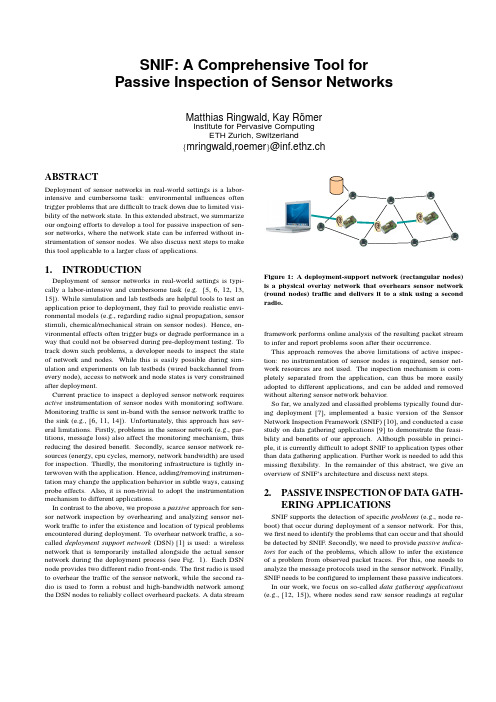
SNIF:A Comprehensive Tool forPassive Inspection of Sensor NetworksMatthias Ringwald,Kay R¨omerInstitute for Pervasive ComputingETH Zurich,Switzerland{mringwald,roemer}@inf.ethz.chABSTRACTDeployment of sensor networks in real-world settings is a labor-intensive and cumbersome task:environmental influences oftentrigger problems that are difficult to track down due to limited visi-bility of the network state.In this extended abstract,we summarizeour ongoing efforts to develop a tool for passive inspection of sen-sor networks,where the network state can be inferred without in-strumentation of sensor nodes.We also discuss next steps to make this tool applicable to a larger class of applications.1.INTRODUCTIONDeployment of sensor networks in real-world settings is typi-cally a labor-intensive and cumbersome task(e.g.[5,6,12,13, 15]).While simulation and lab testbeds are helpful tools to test an application prior to deployment,they fail to provide realistic envi-ronmental models(e.g.,regarding radio signal propagation,sensor stimuli,chemical/mechanical strain on sensor nodes).Hence,en-vironmental effects often trigger bugs or degrade performance in a way that could not be observed during pre-deployment testing.To track down such problems,a developer needs to inspect the state of network and nodes.While this is easily possible during sim-ulation and experiments on lab testbeds(wired backchannel from every node),access to network and node states is very constrained after deployment.Current practice to inspect a deployed sensor network requires active instrumentation of sensor nodes with monitoring software. Monitoring traffic is sent in-band with the sensor network traffic to the sink(e.g.,[6,11,14]).Unfortunately,this approach has sev-eral limitations.Firstly,problems in the sensor network(e.g.,par-titions,message loss)also affect the monitoring mechanism,thus reducing the desired benefit.Secondly,scarce sensor network re-sources(energy,cpu cycles,memory,network bandwidth)are used for inspection.Thirdly,the monitoring infrastructure is tightly in-terwoven with the application.Hence,adding/removing instrumen-tation may change the application behavior in subtle ways,causing probe effects.Also,it is non-trivial to adopt the instrumentation mechanism to different applications.In contrast to the above,we propose a passive approach for sen-sor network inspection by overhearing and analyzing sensor net-work traffic to infer the existence and location of typical problems encountered during deployment.To overhear network traffic,a so-called deployment support network(DSN)[1]is used:a wireless network that is temporarily installed alongside the actual sensor network during the deployment process(see Fig.1).Each DSN node provides two different radio front-ends.Thefirst radio is used to overhear the traffic of the sensor network,while the second ra-dio is used to form a robust and high-bandwidth network among the DSN nodes to reliably collect overheard packets.A datastream Figure1:A deployment-support network(rectangular nodes) is a physical overlay network that overhears sensor network (round nodes)traffic and delivers it to a sink using a second radio.framework performs online analysis of the resulting packet stream to infer and report problems soon after their occurrence.This approach removes the above limitations of active inspec-tion:no instrumentation of sensor nodes is required,sensor net-work resources are not used.The inspection mechanism is com-pletely separated from the application,can thus be more easily adopted to different applications,and can be added and removed without altering sensor network behavior.So far,we analyzed and classified problems typically found dur-ing deployment[7],implemented a basic version of the Sensor Network Inspection Framework(SNIF)[10],and conducted a case study on data gathering applications[9]to demonstrate the feasi-bility and benefits of our approach.Although possible in princi-ple,it is currently difficult to adopt SNIF to application types other than data gathering application.Further work is needed to add this missingflexibility.In the remainder of this abstract,we give an overview of SNIF’s architecture and discuss next steps.2.PASSIVE INSPECTION OF DATA GATH-ERING APPLICATIONSSNIF supports the detection of specific problems(e.g.,node re-boot)that occur during deployment of a sensor network.For this, wefirst need to identify the problems that can occur and that should be detected by SNIF.Secondly,we need to provide passive indica-tors for each of the problems,which allow to infer the existence of a problem from observed packet traces.For this,one needs to analyze the message protocols used in the sensor network.Finally, SNIF needs to be configured to implement these passive indicators. In our work,we focus on so-called data gathering applications (e.g.,[12,15]),where nodes send raw sensor readings at regularintervals along a spanning tree across multiple hops to a sink.The reason for our choice is that almost all existing non-trivial deploy-ments are data gathering applications.Below,we willfirst charac-terize data gathering applications in more detail,before presenting typical problems with these applications and matching passive in-dicators.2.1Application ModelSystems for data gathering such as the Extensible Sensing Sys-tem(ESS)[4]need to maintain a spanning tree of the network along which sensor values are routed to the sink.To support neighbor discovery,all nodes broadcast beacon messages at regular inter-vals.Each beacon message contains a sequence number.To dis-cover neighbors,nodes overhear these messages and estimate the quality of incoming links from neighbors based on message loss. Nodes then broadcast link advertisement messages at regular in-tervals,containing a list of neighbors and link quality estimates. Overhearing these messages,nodes compute the bidirectional link quality to decide on a good set of neighbors.To construct a span-ning tree of the network with the sink at the root,nodes broadcast path advertisement messages,containing the quality of their cur-rent path to the sink.Nodes overhearing these messages can then select the neighbor with the best path as their parent and broadcast an according path advertisement message.Finally,data messages are sent from nodes to the sink along the edges of the spanning tree across multiple hops.2.2Problems and IndicatorsA indicator is an observable behavior of a sensor network that hints(in the sense of a heuristic)the existence of a specific problem. We are interested in passive indicators that can be observed purely by overhearing the traffic of the sensor network as this does not require any instrumentation of the sensor nodes.In[7]we studied existing deployments to identify common prob-lems and derived passive indicators for them.We classify problems according to the number of nodes involved into four classes based on existing deployments:node problems that involve only a sin-gle node,link problems that involve two neighboring nodes and the wireless link between them,path problems that involve three or more nodes and a multi-hop path formed by them,and global problems that are properties of the network as a whole.Below,we provide for each category an exemplary problem and passive indi-cators to detect it.Node reboot,as an example for a node problem,causes the se-quence number counter of the affected node to be reset to an initial value(typically zero).Hence,the sequence number contained in beacon messages sent by the node will jump to a smaller value af-ter a reboot with high probability even in case of lost messages, which can serve as an indicator for reboot.An isolated node,as an example for a link problem,has no neighbors in the network topology.An indicator for this problem is that the node is not listed in any link advertisement messages send by other nodes.An orphaned node,as an example for a path problem,has no parent in the routing tree.Such nodes will either send no path an-nouncement messages at all or path announcements contain an infi-nite distance to the sink(depending on the protocol details),which can be used as a passive indicator.A partitioned node,as an example of a global problem,is dis-conneted from the sink,for example due to death of a node on the path.A node is considered as partitioned if all paths from the node to the sink involve dead nodes.This predicate requires an approx-imate view on the network topology which is reconstructed on theFigure2:Architecture of SNIF.base of observed data packets.Periodic checks on the reconstructed topology serve as a passive indicator here.3.SNIFIn this section we outline how passive indicators discussed in the previous section can be implemented in SNIF.For this,consider the architecture of SNIF as depicted in Fig.2,which consists of a deployment support network to overhear sensor network traffic,a packet decoder to access the contents of overheard packets,a data stream processor to analyze packet streams for problems,a decision tree to infer the state of each sensor node,and a user interface to display these states.The key design goal for SNIF is generality that is,it should support passive inspection of a wide variety of sensor network protocols and applications.Below we give an overview of these components.More details can be found in a[10].3.1Deployment Support Network(DSN)To overhear the traffic of multi-hop networks,multiple radios are needed,forming a distributed network sniffer.We use a so-called deployment support network for this purpose,a wireless network of DSN nodes,each of which provides two radios.Our current implementation of a DSN is based on the BTnode Rev.3[2],which provides two radio front-ends:a Zeevo ZV4002 Bluetooth1.2radio which is used as the DSN radio,and a Chipcon CC1000(e.g.,also used on MICA2)which is used as the WSN ing a scatternet formation algorithm,the DSN nodes form a robust Bluetooth scatternet(see[1]for details).A laptop computer with Bluetooth acts as the SNIF sink that connects to a nearby DSN node.This DSN node thereupon acts as the DSN sink and forms the root of an overlay tree spanning the whole DSN.The SNIF sink can send data to DSN nodes down the tree while DSN nodes send overheard packets up the tree to the sink.Time synchronization exploits the fact that Bluetooth uses a TDMA MAC protocol and thus performs clock synchronization in-ternally,providing an interface to read the Bluetooth clock and its offset to the clocks of network neighbors.We use this interface to compute the clock offset of each DSN node to the DSN sink.A detailed description of our time synchronization protocol can be found in[8].3.2Physical Layer and Medium AccessDSN nodes need a receive-only implementation of the physical (PHY)and MAC layers in order to overhear sensor network traffic. Due to the lack of a standard protocol stack,many variants of PHY and MAC are in use in sensor networks.Our generic PHY imple-mentation supports configurable carrier frequency,baud rate,and checksumming details as illustrated in Fig.2.Regarding MAC,we exploit the fact that–regardless of the specific MAC protocol used –a radio packet always has to be preceded by a preamble and a start-of-packet(SOP)delimiter to synchronize sender and receiver. In our generic MAC implementation,every DSN node has its WSN radio turned to receive mode all the time,looking for a preamble followed by the SOP delimiter in the received stream of bits.Once an SOP has been found,payload data and a CRC follow.This way, DSN nodes can receive packets independent of the actual MAC layer used.3.3Packet DecoderAgain,since no standard protocols exist for sensor networks,we need aflexible mechanism to decode overheard packets.Since most programming environments for sensor nodes are based on the C programming language or a dialect of it(e.g.,nesC for TinyOS), it is common to specify message contents as(nested)C structs in the source code of the sensor network application.Our packet de-coder uses an annotated version of such C structs as a description of the packet contents.This way,the user can copy and paste packet descriptions from the source code.The configuration of the packet decoder consists of some global parameters(such as byte order and alignment),type definitions, and one or more C structs.One of these structs is indicated as the default packet layout.Note that such a struct can contain nested other structs,effectively implementing a discriminated union. Fig.2shows an example of a TinyOS message(TOS Msg)hold-ing a beacon data unit if the message type of the TinyOS message equals1.The result of packet decoding is a record consisting of a list of name-value pairs,where each pair holds the name and value of a datafield in the packet.3.4Data Stream ProcessorThe resulting stream of packets is then fed to a data stream pro-cessor to detect any problems with the sensor network.The data stream processor executes operators that take a stream of records as input and produce a different stream of records as output.The out-put of an operator can be connected to the input of other operators, resulting in a directed operator graph.SNIF provides a set of stan-dard operators,e.g.,forfiltering,aggregation over time windows, or merging of multiple streams into one.In addition,application-specific operators to detect specific problems in the sensor network may be required.Fig.2shows an simple operator graph that is used to detect node reboots as described in Sect.2.2.Thefirst op-erator(filter)reads the packet stream generated by the DSN and removes all packets that are not beacon packets.The sec-ond operator(seqReset)remembers the last sequence number received from each node and checks if a newly received sequence number is smaller than the previous one for this node,in which case the node has rebooted unless there was a sequence number wrap-around(i.e.,maximum sequence number has been reached and sequence counter wraps tozero).Figure3:An instance of SNIF’s user interface.3.5Root Cause AnalysisThe next step is to derive the state of each sensor node,which can be either“node ok”or“node has problem X”.Note that the operator graphs mentioned above may concurrently report multiple problems for a single node.In many cases,one of the problems is a consequence of another problem.For example,a node that is dead also has a routing problem.In such cases,we want to report only the primary problem and not secondary problems.For this, we use a decision tree,where each internal node is a decision that refers to the output of an operator graph,and each leaf is a node state.In the example tree depicted in Fig.2,wefirst check(using the output of an operator graph that counts packets received during a time window)if any messages have been received from a node. If not,then the state of this node is set to“node dead”.Otherwise, if we received packets from this node,we next check if this node has any neighbors(using an operator graph that counts the number of neighbors contained in link advertisement packets received from this node).If there are no neighbors,then the node state is set to “node isolated”.Here,the check for node death is above the check for isolation in the decision tree,because a dead node(primary problem)is also isolated(secondary problem).3.6User InterfaceFinally,node states and additional information are displayed in the graphical user interface.The core abstraction implemented by the user interface is a network graph,where nodes and links can be annotated with arbitrary information.The user interface also supports recording and playback of executions.A snapshot of an instance of the user interface is shown in Fig. 3.Here,node color indicates state(green:ok,gray:not covered by DSN,yellow: warning,red:severe problem),detailed node state can displayed by selecting nodes.Thin arcs indicate what a node believes are its neighbors,thick arcs indicate the paths of multi-hop data messages.4.RELATED WORKMost closely related to SNIF is work on active debugging of sen-sor networks,notably Sympathy[6]and Memento[11].However, both systems require instrumentation of sensor nodes and introduce monitoring protocols in-band with the actual sensor network traffic. Also,both tools only support afixed set of problems,while SNIF provides an extensible framework.Tools for sensor network management such as NUCLEUS[14] provide read/write access to various parameters of a sensor node that may be helpful to detect problems.However,this approach also requires active instrumentation of the sensor network.5.NEXT STEPSAs mentioned in Sect.2.1,our current work is focused on data gathering applications.As other types of applications such as track-ing and event detection are deployed,we will analyze experiences gained from deployments and add support for inspection of these applications to SNIF.For this,novel indicators may have to be im-plemented in SNIF.While SNIF supports thisflexibility in principle through composition and parametrization of data stream operators, currently Java code needs to be written and the developer has to be familiar with SNIF internals.One of the next steps is therefore the development of appropriate high-level specification techniques to support more convenient configuration of SNIF for different types of applications.In particular,we envision a graphical notation,al-lowing a user to devise these specifications using a graphical user interface.Ultimately,we want to achieve(semi-)automatic generation of these specifications from application programs.For this,we will work on analyzing high-level declarative program specifications such as SNlog[3].These capture the application semantics in a more direct way than procedural programs,such that it may be pos-sible to derive SNIF configurations without explicit annotations.6.ACKNOWLEDGMENTSThe work presented in this paper was partially supported by the National Competence Center in Research on Mobile Information and Communication Systems(NCCR-MICS),a center supported by the Swiss National Science Foundation under grant number 5005-67322.7.REFERENCES[1]J.Beutel,M.Dyer,L.Meier,and L.Thiele.ScalableTopology Control for Deployment-Sensor Networks.InIPSN2005.[2]BTnodes.A Distributed Environment for Prototyping AdHoc Networks.www.btnode.ethz.ch.[3]D.C.Chu,L.Popa,A.Tavakoli,J.M.Hellerstein,P.Levis,S.Shenker,and I.Stoica.The design and implementation ofa declarative sensor network system.Technical ReportUCB/EECS-2006-132,EECS Department,UC Berkeley,October2006.[4]R.Guy,B.Greenstein,J.Hicks,R.Kapur,N.Ramanathan,T.Schoellhammer,T.Stathopoulos,K.Weeks,K.Chang,L.Girod,and D.Estrin.Experiences with the ExtensibleSensing System ESS.Technical Report61,CENS,2006. [5]P.Padhy,K.Martinez,A.Riddoch,H.L.R.Ong,and J.K.Hart.Glacial Environment Monitoring using SensorNetworks.In REALWSN2005.[6]N.Ramanathan,K.Chang,R.Kapur,L.Girod,E.Kohler,and D.Estrin.Sympathy for the Sensor Network Debugger.In SenSys2005.[7]M.Ringwald and K.R¨o mer.Deployment of SensorNetworks:Problems and Passive Inspection.In WISES2007.[8]M.Ringwald and K.R¨o mer.Practical Time Synchronizationfor Bluetooth Scatternets.In BROADNETS2007.[9]M.Ringwald,K.R¨o mer,and A.Vialetti.Passive Inspectionof Sensor Networks.In DCOSS2007.[10]M.Ringwald,K.R¨o mer,and A.Vialetti.SNIF:SensorNetwork Inspection Framework.Technical Report535,Departement of Computer Science,ETH Zurich,2006. [11]S.Rost and H.Balakrishnan.Memento:A HealthMonitoring System for Wireless Sensor Networks.InSECON2006.[12]R.Szewcyk,A.Mainwaring,J.Polastre,J.Anderson,andD.Culler.An Analysis of a Large Scale Habitat MonitoringApplication.In SenSys2004.[13]J.Tateson,C.Roadknight,A.Gonzalez,S.Fitz,N.Boyd,C.Vincent,and I.Marshall.Real World Issues in Deployinga Wireless Sensor Network for Oceanography.In REALWSN2005.[14]G.Tolle and D.Culler.Design of anApplication-Cooperative Management System for WirelessSensor Networks.In EWSN2005.[15]G.Tolle,J.Polastre,R.Szewczyk,D.Culler,N.Turner,K.Tu,S.Burgess,T.Dawson,P.Buonadonna,D.Gay,andW.Hong.A Macroscope in the Redwoods.In SenSys2005.。

CCF推荐的国际学术会议和期刊目录修订版发布CCF(China Computer Federation中国计算机学会)于2010年8月发布了第一版推荐的国际学术会议和期刊目录，一年来，经过业内专家的反馈和修订，于日前推出了修订版，现将修订版予以发布。

本次修订对上一版内容进行了充实，一些会议和期刊的分类排行进行了调整，目录包括：计算机科学理论、计算机体系结构与高性能计算、计算机图形学与多媒体、计算机网络、交叉学科、人工智能与模式识别、软件工程/系统软件/程序设计语言、数据库/数据挖掘/内容检索、网络与信息安全、综合刊物等方向的国际学术会议及期刊目录，供国内高校和科研单位作为学术评价的参考依据。

目录中，刊物和会议分为A、B、C三档。

A类表示国际上极少数的顶级刊物和会议，鼓励我国学者去突破；B类是指国际上著名和非常重要的会议、刊物，代表该领域的较高水平，鼓励国内同行投稿；C类指国际上重要、为国际学术界所认可的会议和刊物。

这些分类目录每年将学术界的反馈和意见，进行修订，并逐步增加研究方向。

中国计算机学会推荐国际学术刊物（网络/信息安全）一、 A类序号刊物简称刊物全称出版社网址1. TIFS IEEE Transactions on Information Forensics andSecurity IEEE /organizations/society/sp/tifs.html2. TDSC IEEE Transactions on Dependable and Secure ComputingIEEE /tdsc/3. TISSEC ACM Transactions on Information and SystemSecurity ACM /二、 B类序号刊物简称刊物全称出版社网址1. Journal of Cryptology Springer /jofc/jofc.html2. Journal of Computer SecurityIOS Press /jcs/3. IEEE Security & Privacy IEEE/security/4. Computers &Security Elsevier http://www.elsevier.nl/inca/publications/store/4/0/5/8/7/7/5. JISecJournal of Internet Security NahumGoldmann. /JiSec/index.asp6. Designs, Codes andCryptography Springer /east/home/math/numbers?SGWID=5 -10048-70-35730330-07. IET Information Security IET /IET-IFS8. EURASIP Journal on InformationSecurity Hindawi /journals/is三、C类序号刊物简称刊物全称出版社网址1. CISDA Computational Intelligence for Security and DefenseApplications IEEE /2. CLSR Computer Law and SecurityReports Elsevier /science/journal/026736493. Information Management & Computer Security MCB UniversityPress /info/journals/imcs/imcs.jsp4. Information Security TechnicalReport Elsevier /locate/istr中国计算机学会推荐国际学术会议（网络/信息安全方向）一、A类序号会议简称会议全称出版社网址1. S&PIEEE Symposium on Security and Privacy IEEE /TC/SP-Index.html2. CCSACM Conference on Computer and Communications Security ACM /sigs/sigsac/ccs/3. CRYPTO International Cryptology Conference Springer-Verlag /conferences/二、B类序号会议简称会议全称出版社网址1. SecurityUSENIX Security Symposium USENIX /events/2. NDSSISOC Network and Distributed System Security Symposium Internet Society /isoc/conferences/ndss/3. EurocryptAnnual International Conference on the Theory and Applications of Cryptographic Techniques Springer /conferences/eurocrypt2009/4. IH Workshop on Information Hiding Springer-Verlag /~rja14/ihws.html5. ESORICSEuropean Symposium on Research in Computer Security Springer-Verlag as.fr/%7Eesorics/6. RAIDInternational Symposium on Recent Advances in Intrusion Detection Springer-Verlag /7. ACSACAnnual Computer Security Applications ConferenceIEEE /8. DSNThe International Conference on Dependable Systems and Networks IEEE/IFIP /9. CSFWIEEE Computer Security Foundations Workshop /CSFWweb/10. TCC Theory of Cryptography Conference Springer-Verlag /~tcc08/11. ASIACRYPT Annual International Conference on the Theory and Application of Cryptology and Information Security Springer-Verlag /conferences/ 12. PKC International Workshop on Practice and Theory in Public Key Cryptography Springer-Verlag /workshops/pkc2008/三、 C类序号会议简称会议全称出版社网址1. SecureCommInternational Conference on Security and Privacy in Communication Networks ACM /2. ASIACCSACM Symposium on Information, Computer and Communications Security ACM .tw/asiaccs/3. ACNSApplied Cryptography and Network Security Springer-Verlag /acns_home/4. NSPWNew Security Paradigms Workshop ACM /current/5. FC Financial Cryptography Springer-Verlag http://fc08.ifca.ai/6. SACACM Symposium on Applied Computing ACM /conferences/sac/ 7. ICICS International Conference on Information and Communications Security Springer /ICICS06/8. ISC Information Security Conference Springer /9. ICISCInternational Conference on Information Security and Cryptology Springer /10. FSE Fast Software Encryption Springer http://fse2008.epfl.ch/11. WiSe ACM Workshop on Wireless Security ACM /~adrian/wise2004/12. SASN ACM Workshop on Security of Ad-Hoc and Sensor Networks ACM /~szhu/SASN2006/13. WORM ACM Workshop on Rapid Malcode ACM /~farnam/worm2006.html14. DRM ACM Workshop on Digital Rights Management ACM /~drm2007/15. SEC IFIP International Information Security Conference Springer http://sec2008.dti.unimi.it/16. IWIAIEEE International Information Assurance Workshop IEEE /17. IAWIEEE SMC Information Assurance Workshop IEEE /workshop18. SACMATACM Symposium on Access Control Models and Technologies ACM /19. CHESWorkshop on Cryptographic Hardware and Embedded Systems Springer /20. CT-RSA RSA Conference, Cryptographers' Track Springer /21. DIMVA SIG SIDAR Conference on Detection of Intrusions and Malware and Vulnerability Assessment IEEE /dimva200622. SRUTI Steps to Reducing Unwanted Traffic on the Internet USENIX /events/23. HotSecUSENIX Workshop on Hot Topics in Security USENIX /events/ 24. HotBots USENIX Workshop on Hot Topics in Understanding Botnets USENIX /event/hotbots07/tech/25. ACM MM&SEC ACM Multimedia and Security Workshop ACM。

专利名称：基于深度复数网络的智能反射面系统的反射系数估计方法
专利类型：发明专利
发明人：周鑫,殷锐
申请号：CN202111559522.1
申请日：20211220
公开号：CN114499711A
公开日：
20220513
专利内容由知识产权出版社提供
摘要：本发明提供了一种基于深度复数网络的智能反射面系统的反射系数估计方法，其特征在于，所述深度复数网络应用于智能反射面系统中，单天线用户的情况下，通过将仿真生成的信道参数和反射系数标签分别作为输入和输出训练深度复数网络，此网络可在已知信道参数的基础上输出反射系数的取值。

本发明所提出的基于深度复数网络的智能反射面系统的反射系数估计在与传统的基于半定松弛算法的反射系数估计方案相比，不仅大大降低了计算复杂度，而且极大的降低了系统的功耗，为移动通信网络的绿色可持续发展提供了可能。

申请人：浙江大学
地址：310058 浙江省杭州市西湖区余杭塘路866号
国籍：CN
更多信息请下载全文后查看。

光纤传感会议ofs学术poster展示模板-回复光纤传感会议（OFS）学术Poster展示模板光纤传感（OFS）是一种应用光纤技术进行传感和监测的方法，通过利用光纤的特殊传输特性，有效地实现了高灵敏度、高分辨率和远程监测。

光纤传感在各种领域中得到了广泛的应用，包括环境监测、医疗诊断和结构监测等。

在光纤传感会议（OFS）中，学术Poster展示是研究人员分享研究成果的一种常见形式。

本文将以中括号内的内容为主题，详细解析光纤传感会议（OFS）学术Poster展示模板，并针对每一步进行深入讨论。

1. 研究背景及目的在这一部分，介绍你的研究背景和目的。

解释为什么你选择了这个话题，并说明你的研究对于光纤传感领域的意义。

2. 研究方法在这一部分，介绍你所采用的研究方法。

这可能包括实验设计、所使用的设备和技术等等。

详细描述你的方法，让读者了解你的实验过程。

3. 结果分析在这一部分，展示你的研究结果并进行详细的分析。

使用图表、图像和数据来支持你的观点，并解释你得出的结论。

此外，你还可以提供一些额外的实验结果或图表来支持你的主要结论。

4. 创新性和应用价值在这一部分，阐明你的研究的创新性和应用价值。

解释你的研究结果对于光纤传感领域的重要性，并讨论你的研究结果可能对其他领域的影响。

5. 讨论与展望在这一部分，对你的研究结果进行全面的讨论，并提出进一步的展望。

讨论你的结果与现有文献的一致性或差异性，并解释你的研究的局限性。

最后，提出你的下一步研究计划，让读者对你未来的研究感到期待。

以上是针对光纤传感会议（OFS）学术Poster展示的模板和详细步骤的讲解。

根据这个模板，你可以编写一篇1500-2000字的文章，一步一步回答各个部分的问题。

确保你的内容清晰、有条理，并使用图表、图像和数据来支持你的观点。

最后，不要忘记为读者提供一个全面的讨论和未来展望，以便他们对你的研究结果和未来计划有更深入的了解。

祝你在光纤传感会议（OFS）学术Poster展示中取得成功！。

ｄｏｉ：１０．３９６９／ｊ．ｉｓｓｎ．１００３－３１１４．２０２４．０２．００２引用格式：张建华，张骥威，张宇翔，等．面向６Ｇ的ＲＩＳ信道测量与建模研究进展［Ｊ］．无线电通信技术，２０２４，５０（２）：２２７－２３７．［ＺＨＡＮＧＪｉａｎｈｕａ，ＺＨＡＮＧＪｉｗｅｉ，ＺＨＡＮＧＹｕｘｉａｎｇ，ｅｔａｌ．ＡｄｖａｎｃｅｍｅｎｔｓｉｎＲＩＳＣｈａｎｎｅｌＭｅａｓｕｒｅｍｅｎｔａｎｄＭｏｄｅｌｉｎｇｆｏｒ６Ｇ［Ｊ］．ＲａｄｉｏＣｏｍｍｕｎｉｃａｔｉｏｎｓＴｅｃｈｎｏｌｏｇｙ，２０２４，５０（２）：２２７－２３７．］面向６Ｇ的ＲＩＳ信道测量与建模研究进展张建华１，张骥威１，张宇翔２，巩汇文１，田　磊１（１．北京邮电大学信息与通信工程学院，北京１００８７６；２．北京邮电大学集成电路学院，北京１００８７６）摘　要：智能超表面（ＲｅｃｏｎｆｉｇｕｒａｂｌｅＩｎｔｅｌｌｉｇｅｎｔＳｕｒｆａｃｅ，ＲＩＳ）技术被认为是６Ｇ中很有应用前景的技术。

ＲＩＳ信道研究对于ＲＩＳ辅助通信系统的技术创新和性能评价至关重要。

综述了ＲＩＳ信道的测量与建模研究进展，总结了基于矢量网络分析仪（ＶｅｃｔｏｒＮｅｔｗｏｒｋＡｎａｌｙｚｅｒ，ＶＮＡ）的频域测量和基于滑动相关的时域测量两种信道测量方法。

介绍了基于时域的ＲＩＳ信道测量平台，并对目前的测量活动进行了总结。

分析了ＲＩＳ信道中的阵元反射系数、散射方向图和级联路径损耗三个特性。

总结了ＲＩＳ信道统计性建模、确定性建模和混合型建模的方法，给出了一种基于现有５Ｇ标准的３Ｄ几何统计性信道模型（Ｇｅｏｍｅｔｒｉｃ ＢａｓｅｄＳｔｏｃｈａｓｔｉｃＭｏｄｅｌ，ＧＢＳＭ）扩展的ＲＩＳ信道建模方法，以及基于此方法的ＲＩＳ信道仿真平台。

展望了ＲＩＳ信道测量和建模研究面临的挑战和未来的研究方向。

关键词：智能超表面；信道测量；信道建模；３Ｄ几何统计性信道建模中图分类号：ＴＮ９２９．５ 文献标志码：Ａ 开放科学（资源服务）标识码（ＯＳＩＤ）：文章编号：１００３－３１１４（２０２４）０２－０２２７－１１ＡｄｖａｎｃｅｍｅｎｔｓｉｎＲＩＳＣｈａｎｎｅｌＭｅａｓｕｒｅｍｅｎｔａｎｄＭｏｄｅｌｉｎｇｆｏｒ６ＧＺＨＡＮＧＪｉａｎｈｕａ１，ＺＨＡＮＧＪｉｗｅｉ１，ＺＨＡＮＧＹｕｘｉａｎｇ２，ＧＯＮＧＨｕｉｗｅｎ１，ＴＩＡＮＬｅｉ１（１．ＳｃｈｏｏｌｏｆＩｎｆｏｒｍａｔｉｏｎａｎｄＣｏｍｍｕｎｉｃａｔｉｏｎＥｎｇｉｎｅｅｒｉｎｇ，ＢｅｉｊｉｎｇＵｎｉｖｅｒｓｉｔｙｏｆＰｏｓｔｓａｎｄＴｅｌｅｃｏｍｍｕｎｉｃａｔｉｏｎｓ，Ｂｅｉｊｉｎｇ１００８７６，Ｃｈｉｎａ；２．ＳｃｈｏｏｌｏｆＩｎｔｅｇｒａｔｅｄＣｉｒｃｕｉｔｓ，ＢｅｉｊｉｎｇＵｎｉｖｅｒｓｉｔｙｏｆＰｏｓｔｓａｎｄＴｅｌｅｃｏｍｍｕｎｉｃａｔｉｏｎｓ，Ｂｅｉｊｉｎｇ１００８７６，Ｃｈｉｎａ）Ａｂｓｔｒａｃｔ：ＲｅｃｏｎｆｉｇｕｒａｂｌｅＩｎｔｅｌｌｉｇｅｎｔＳｕｒｆａｃｅ（ＲＩＳ）ｔｅｃｈｎｏｌｏｇｙｉｓｃｏｎｓｉｄｅｒｅｄａｐｒｏｍｉｓｉｎｇａｐｐｌｉｃａｔｉｏｎｉｎ６Ｇ．ＴｈｅｒｅｓｅａｒｃｈｏｎＲＩＳｃｈａｎｎｅｌｓｉｓｃｒｕｃｉａｌｆｏｒｔｅｃｈｎｏｌｏｇｉｃａｌｉｎｎｏｖａｔｉｏｎａｎｄｐｅｒｆｏｒｍａｎｃｅｅｖａｌｕａｔｉｏｎｏｆＲＩＳａｓｓｉｓｔｅｄｃｏｍｍｕｎｉｃａｔｉｏｎｓｙｓｔｅｍｓ．ＴｈｉｓａｒｔｉｃｌｅｒｅｖｉｅｗｓｔｈｅｒｅｓｅａｒｃｈｐｒｏｇｒｅｓｓｉｎｍｅａｓｕｒｅｍｅｎｔａｎｄｍｏｄｅｌｉｎｇｏｆＲＩＳｃｈａｎｎｅｌｓ．Ｗｅｓｕｍｍａｒｉｚｅｄｔｗｏｃｈａｎｎｅｌｍｅａｓｕｒｅｍｅｎｔｍｅｔｈｏｄｓ，ｆｒｅｑｕｅｎｃｙｄｏ ｍａｉｎｍｅａｓｕｒｅｍｅｎｔｂａｓｅｄｏｎＶｅｃｔｏｒＮｅｔｗｏｒｋＡｎａｌｙｚｅｒ（ＶＮＡ）ａｎｄｔｉｍｅ ｄｏｍａｉｎｍｅａｓｕｒｅｍｅｎｔｂａｓｅｄｏｎｓｌｉｄｉｎｇｃｏｒｒｅｌａｔｉｏｎ．Ｗｅｉｎｔｒｏ ｄｕｃｅｄａｔｉｍｅ ｄｏｍａｉｎＲＩＳｃｈａｎｎｅｌｍｅａｓｕｒｅｍｅｎｔｐｌａｔｆｏｒｍａｎｄｓｕｍｍａｒｉｚｅｄｃｕｒｒｅｎｔｍｅａｓｕｒｅｍｅｎｔａｃｔｉｖｉｔｉｅｓ．Ｔｈｒｅｅｃｈａｒａｃｔｅｒｉｓｔｉｃｓｏｆｅｌｅｍｅｎｔｒｅｆｌｅｃｔｉｏｎｃｏｅｆｆｉｃｉｅｎｔ，ｓｃａｔｔｅｒｉｎｇｐａｔｔｅｒｎ，ａｎｄｃａｓｃａｄｅｄｐａｔｈｌｏｓｓｉｎＲＩＳｃｈａｎｎｅｌｓａｒｅａｎａｌｙｚｅｄ．ＡｓｕｍｍａｒｙｏｆＲＩＳｃｈａｎｎｅｌｍｏｄｅｌ ｉｎｇｍｅｔｈｏｄｓ，ｉｎｃｌｕｄｉｎｇｓｔａｔｉｓｔｉｃａｌｍｏｄｅｌｉｎｇ，ｄｅｔｅｒｍｉｎｉｓｔｉｃｍｏｄｅｌｉｎｇ，ａｎｄｈｙｂｒｉｄｍｏｄｅｌｉｎｇ，ｉｓｐｒｅｓｅｎｔｅｄ．ＡｎｅｘｔｅｎｄｅｄＲＩＳｃｈａｎｎｅｌｍｏｄｅｌｉｎｇｍｅｔｈｏｄｂａｓｅｄｏｎｅｘｉｓｔｉｎｇ５Ｇｓｔａｎｄａｒｄ ｓ３ＤＧｅｏｍｅｔｒｉｃ ＢａｓｅｄＳｔｏｃｈａｓｔｉｃＭｏｄｅｌ（ＧＢＳＭ）ｉｓｐｒｏｐｏｓｅｄ，ａｓｗｅｌｌａｓａｎＲＩＳｃｈａｎ ｎｅｌｓｉｍｕｌａｔｉｏｎｐｌａｔｆｏｒｍｂａｓｅｄｏｎｔｈｉｓｍｅｔｈｏｄ．Ｆｉｎａｌｌｙ，ｃｈａｌｌｅｎｇｅｓａｎｄｆｕｔｕｒｅｒｅｓｅａｒｃｈｄｉｒｅｃｔｉｏｎｓｆａｃｅｄｂｙＲＩＳｃｈａｎｎｅｌｍｅａｓｕｒｅｍｅｎｔａｎｄｍｏｄｅｌｉｎｇｒｅｓｅａｒｃｈｗｅｒｅｄｉｓｃｕｓｓｅｄ．Ｋｅｙｗｏｒｄｓ：ＲＩＳ；ｃｈａｎｎｅｌｍｅａｓｕｒｅｍｅｎｔ；ｃｈａｎｎｅｌｍｏｄｅｌｉｎｇ；３ＤＧＢＳＭ收稿日期：２０２３－１１－２７基金项目：国家重点研发计划（２０２３ＹＦＢ２９０４８０５）；国家自然科学基金青年科学基金（６２１０１０６９，６２２０１０８７）；国家自然科学基金重点项目（９２１６７２０２）；国家杰出青年科学基金（６１９２５１０２）ＦｏｕｎｄａｔｉｏｎＩｔｅｍ：ＮａｔｉｏｎａｌＫｅｙＲ＆ＤＰｒｏｇｒａｍｏｆＣｈｉｎａ（２０２３ＹＦＢ２９０４８０５）；ＹｏｕｎｇＳｃｉｅｎｔｉｓｔｓＦｕｎｄｏｆｔｈｅＮａｔｉｏｎａｌＮａｔｕｒａｌＳｃｉｅｎｃｅＦｏｕｎｄａｔｉｏｎｏｆＣｈｉｎａ（６２１０１０６９，６２２０１０８７）；ＫｅｙＰｒｏｇｒａｍｏｆＮａｔｉｏｎａｌＮａｔｕｒａｌＳｃｉｅｎｃｅＦｏｕｎｄａｔｉｏｎｏｆＣｈｉｎａ（９２１６７２０２）；ＮａｔｉｏｎａｌＳｃｉｅｎｃｅＦｕｎｄｆｏｒＤｉｓｔｉｎｇｕｉｓｈｅｄＹｏｕｎｇＳｃｈｏｌａｒｓ（６１９２５１０２）０　引言随着５Ｇ移动通信系统已在全球范围内部署，６Ｇ移动通信技术的研究正在广泛开展，预计在２０３０年实现商用［１］。