ansys桁架屈曲分析实例

(1) 进入ANSYS(设定工作目录和工作文件)1) 进入ANSYS菜单路径“程序>ANSYS >ANSYS10.0”2) 设置工作文件名菜单路径“file > Change Jobname”，弹出“Change Jobname”对话框，输入“CYKLink”，单击【OK】确定并关闭对话框。

(2) 设置计算类型菜单路径“ANSYS Main Menu: Preferences…”，在弹出的对话框中选择“Structural”，单击【OK】确定并关闭对话框。

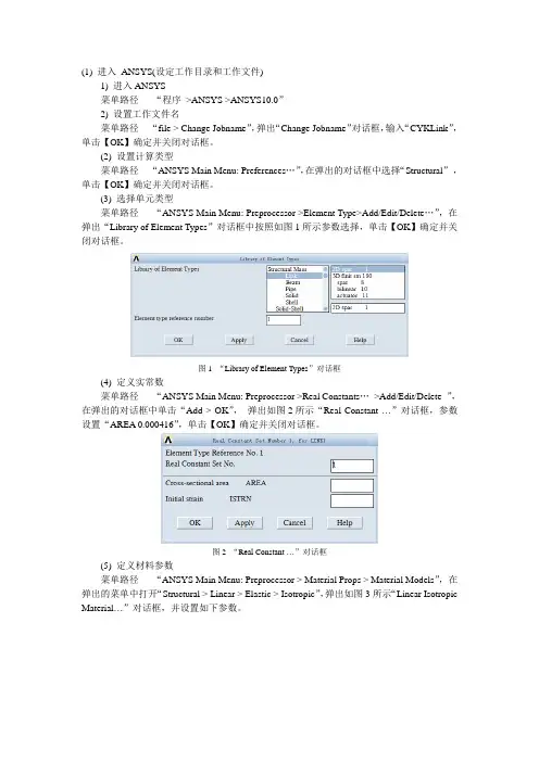
(3) 选择单元类型菜单路径“ANSYS Main Menu: Preprocessor >Element Type>Add/Edit/Delete…”，在弹出“Library of Element Types”对话框中按照如图1所示参数选择，单击【OK】确定并关闭对话框。

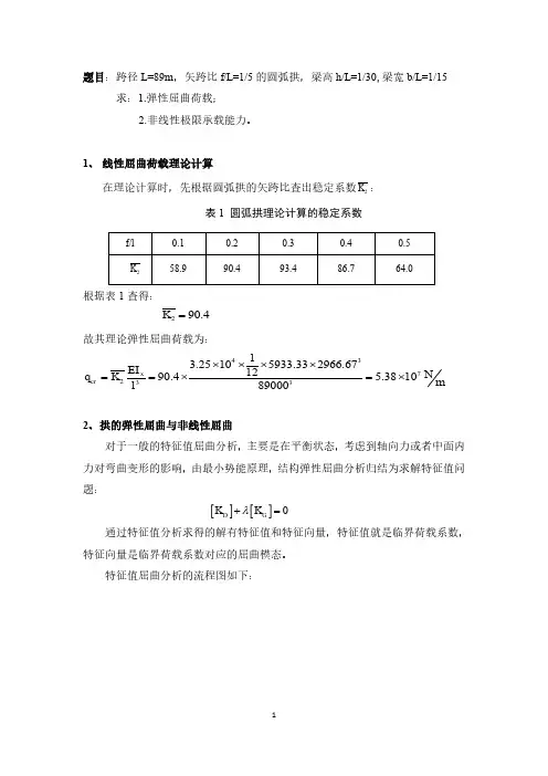
图1 “Library of Element Types”对话框(4) 定义实常数菜单路径“ANSYS Main Menu: Preprocessor >Real Constants…>Add/Edit/Delete ”，在弹出的对话框中单击“Add > OK”，弹出如图2所示“Real Constant …”对话框，参数设置“AREA 0.000416”，单击【OK】确定并关闭对话框。

图2 “Real Constant …”对话框(5) 定义材料参数菜单路径“ANSYS Main Menu: Preprocessor > Material Props > Material Models”，在弹出的菜单中打开“Structural > Linear > Elastic > Isotropic”，弹出如图3所示“Linear Isotropic Material…”对话框，并设置如下参数。

图3 “Linear Isotropic Material…”对话框图4 “Beam Tool”对话框(6) 定义梁的截面菜单路径“ANSYS Main Menu: Preprocessor > Sections > Beam > Common Sections”，弹出如图4所示“Beam Tool”对话框，并按照图4设置，单击【OK】确定关闭对话框。

题目：跨径L=89m ，矢跨比f/L =1/5的圆弧拱，梁高h/L =1/30,梁宽b/L =1/15 求：1.弹性屈曲荷载；2.非线性极限承载能力。

1、 线性屈曲荷载理论计算在理论计算时，先根据圆弧拱的矢跨比查出稳定系数2K ：表1 圆弧拱理论计算的稳定系数根据表1查得：290.4K =故其理论弹性屈曲荷载为：43723313.25105933.332966.671290.4 5.381089000xcr EI N q K m l ⨯⨯⨯⨯==⨯=⨯2、拱的弹性屈曲与非线性屈曲对于一般的特征值屈曲分析，主要是在平衡状态，考虑到轴向力或者中面内力对弯曲变形的影响，由最小势能原理，结构弹性屈曲分析归结为求解特征值问题：通过特征值分析求得的解有特征值和特征向量，特征值就是临界荷载系数，特征向量是临界荷载系数对应的屈曲模态。

特征值屈曲分析的流程图如下：[][]0D G KK λ+=图1 弹性屈曲分析流程图非线性屈曲分析是考虑结构平衡受扰动（初始缺陷、荷载扰动）的非线性静力分析，该分析是一直加载到结构极限承载状态的全过程分析，分析中可以综合考虑材料塑性和几何非线性。

结构非线性屈曲分析归结为求解矩阵方程：非线性屈曲分析的流程图如下：图2 非线性屈曲分析流程图[][](){}{}DGK K F δ+=3、非线性方程组求解方法（1）增量法增量法的实质是用分段线性的折线去代替非线性曲线。

增量法求解时将荷载分成许多级荷载增量，每次施加一个荷载增量。

在一个荷载增量中假定刚度矩阵保持不变，在不同的荷载增量中，刚度矩阵可以有不同的数值，并与应力应变关系相对应。

（2）迭代法迭代法是通过调整直线斜率对非线性曲线的逐渐逼近。

迭代法求解时每次迭代都将总荷载全部施加到结构上，取结构变形前的刚度矩阵，求得结构位移并对结构的几何形态进行修正，再用此时的刚度矩阵及位移增量求得内力增量，并进一步得到总的内力。

（3）混合法混合法是增量法和迭代法的混合使用。

ansys桁架结构分析实例平面桁架的静力分析摘要：近些年来，ANSYS 工程软件在工程领域内运用的很多，在分析线性有限元模型上比其他软件更具有优势。

而在ANSYS 软件中最常用的是线性静力分析，尽管很多的材料不一样，但结果确基本一致。

本文主要是要对平面桁架进行静力分析。

关键字：线性；桁架；有限元；结构The plane truss static analysisAbstract ：ANSYS engineering software engineering field use in recent years, a lot, in the analysis of linear finite element model on more than any other software advantages. The most commonly used in ANSYS linear static analysis, although a lot of the material is not the same, but the result was consistent. This article is mainly for static analysis of plane truss.Key words：Linear; truss; finite element; structure1. 引言结构分析的四个基本步骤是：创建几何模型、生成有限元模型、加载与求解、结果评价与分析。

具体步骤与结构分析类型有关，并且有些步骤可以省略或相互之间交叉，如简单结构的几何模型创建过程可省略而直接创建有限元模型，加载可在处理层也可以在求阶层等，需要根据具体情况以便利原则而定。

2主要步骤结构线性静力分析步骤为：2.1创建几何模型（1）清楚当前数据库。

回到开始层：FINISH 命令。

清楚数据库的操作步骤要在开始层。

清楚数据库：/CLEAR命令。

ANSYS桁架优化分析实例优化分析的示例（GUI方法）在本例中，用一阶方法进行优化分析。

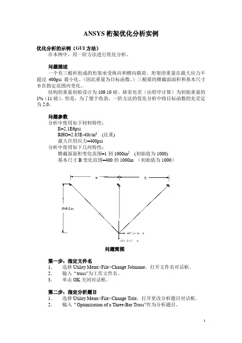
问题描述一个有三根杆组成的珩架承受纵向和横向载荷。

珩架的重量在最大应力不超过400psi最小化。

（因此重量为目标函数。

）三根梁的横截面面积和基本尺寸Ｂ在指定范围内变化。

结构的重量初始设计为109.10磅。

缺省允差（由程序计算）为初始重量的1%（11磅）。

但是，为了便于收敛，一阶方法的优化分析中将目标函数的允差定为2.0。

问题参数分析中使用如下材料特性：E=2.1E6psiRHO=2.85E-4lb/in3(比重)最大许用应力=400psi分析中使用如下几何特性：横截面面积变化范围=1到1000in2(初始值为1000)基本尺寸B变化范围=400到1000in （初始值为1000）问题简图第一步：指定文件名1．选择Utility Menu>File>Change Jobname，打开文件名对话框。

2．输入“truss”为工作文件名。

3．单击OK关闭对话框。

第二步：指定分析题目1．选择Utility Menu>File>Change Title，打开更改分析题目对话框。

2．输入“Optimization of a Three-Bar Truss”作为分析题目。

第三步：定义参数初始值1．选择Utility Menu>Parameters>Scalar Parameters，打开数值参数对话框。

在选择区域中输入下列内容：B=1000 按ENTER键A1=1000 按ENTER键A2=1000 按ENTER键A3=1000 单击OK。

参数将在菜单中显示出来。

2．在数值参数对话框中单击OK。

第四步：定义单元类型1．选择Main Menu>Preprocessor>Element Type>Add/Edit/Delete，打开单元类型对话框。

2．在单元类型库对话框中单击Add。

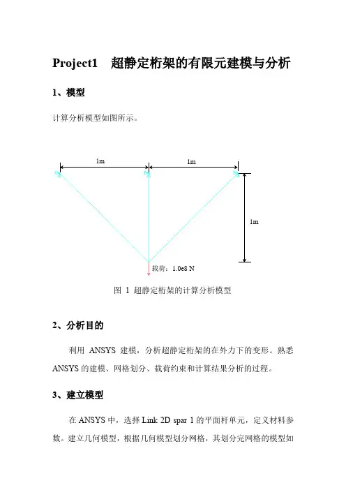
Project1 超静定桁架的有限元建模与分析1、模型计算分析模型如图所示。

载荷：1.0e8N图1 超静定桁架的计算分析模型2、分析目的利用ANSYS建模，分析超静定桁架的在外力下的变形。

熟悉ANSYS的建模、网格划分、载荷约束和计算结果分析的过程。

3、建立模型在ANSYS中，选择Link 2D spar 1的平面杆单元，定义材料参数。

建立几何模型，根据几何模型划分网格，其划分完网格的模型如图2所示图 2 网格模型4、载荷工况1)分别给桁架的非公共端施加X、Y向的约束。

2)在桁架的公共端施加沿Y方向1.0e8 N的载荷。

5、约束处理在ANSYS中，按载荷工况中的要求施加载荷。

其模型如下图3所示。

图 3 模型约束6、结果评价首先分析桁架的变形，其变形如图4和图5下所示。

图 4 变形图由图可知，桁架最大变形DMX=0.112e-03m。

其DOF Solusion-Y向变形如图5 DOF Solution-Y图5 DOF Solution-Y所示图 5 DOF Solution-Y从图中可以看出铰接的应力较为集中，是桁架的危险区域。

Project2 超静定梁的计算分析1、模型计算分析模型如图6所示：梁承受均布载荷：1.0e5 Pa图6超静定梁的计算分析模型2、分析目的利用ANSYS建模，分析超静定桁架的在外力下的变形。

熟悉ANSYS的建模、网格划分、载荷约束和计算结果分析的过程。

3、建立模型在ANSYS中，选择Beam tapered 44单元，定义材料参数。

建立几何模型，根据几何模型划分网格，其划分完网格的模型如错误！未找到引用源。

和错误！未找到引用源。

错误！未找到引用源。

所示。

图7 X向俯视图图8 X向正视图4、载荷工况1)给两端点和中点施加约束。

2)在Y方向施加100000N的载荷5、约束处理在ANSYS中，按载荷工况中的要求施加载荷。

其模型如下图所示。

图9 模型约束6、结果评价计算后模型的变形，如图10所示：图10 变形图从图中可以看出，最大变形量DMX=0.149046m。

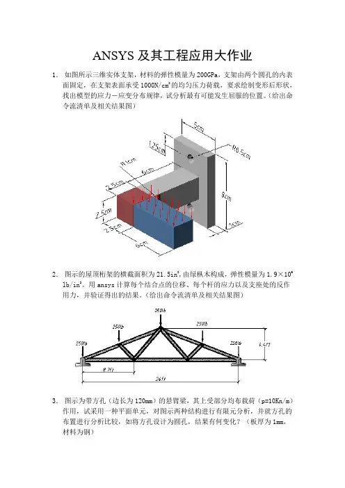
ANSYS及其工程应用大作业1．如图所示三维实体支架，材料的弹性模量为200GPa，支架由两个圆孔的内表面固定，在支架表面承受1000N/cm2的均匀压力荷载，要求绘制变形后形状，找出模型的应力－应变分布规律，试分析最有可能发生屈服的位置。

（给出命令流清单及相关结果图）2．图示的屋顶桁架的横截面积为21.5in2,由绿枞木构成，弹性模量为1.9×106 lb/in2。

用ansys计算每个结合点的位移、每个杆的应力以及支座处的反作用力，并验证得出的结果。

（给出命令流清单及相关结果图）3．图示为带方孔（边长为120mm）的悬臂梁，其上受部分均布载荷（p=10Kn/m）作用，试采用一种平面单元，对图示两种结构进行有限元分析，并就方孔的布置进行分析比较，如将方孔设计为圆孔，结果有何变化？（板厚为1mm，材料为钢）4．如图（a）所示简支吊车梁，梁上有移动荷载以1.0s/m的速度从梁的一端移动到另一端，计算在此过程中吊车梁的位移和应力响应。

其中，梁材料为钢材，弹性模量为2.0×1011Pa，波松比为0.3，密度为7800kg/m3，采用焊接“工”字型组合截面，如图（b）所示，其中W1=150mm，W2=300mm，T1=20mm，T2=10mm。

(a) (b)5．如图所示，一根直的细长悬臂梁，一端固定一端自由。

在自由端施加P=1lb 的载荷。

弹性模量=1.0e4psi，泊松比=0.0；L=100in，H=5in，B=2in；对该悬臂梁做特征值屈曲分析，并进行非线性载荷和变形研究。

研究目标为确定梁发生分支点失稳（标志为侧向的大位移）的临界载荷。

6．请用Ansys中的三维梁单元为下图所示结构的各部分设计横断面尺寸。

要求用空心管。

该结构用于支撑红绿灯，它所承受的风力为80mile/hour,红绿灯灯箱重10kg。

请写一份简要报告，叙述自己的最终设计。

计算分析报告应包括以下部分：A、问题描述及数学建模；B、有限元建模（单元选择、结点布置及规模、网格划分方案、载荷及边界条件处理、求解控制）C、计算结果及结果分析（位移分析、应力分析、正确性分析评判）D、多方案计算比较（结点规模增减对精度的影响分析、单元改变对精度的影响分析、不同网格划分方案对结果的影响分析等）ANSYS及其工程应用大作业7．如图所示三维实体支架，材料的弹性模量为200GPa，支架由两个圆孔的内表面固定，在支架表面承受1000N/cm2的均匀压力荷载，要求绘制变形后形状，找出模型的应力－应变分布规律，试分析最有可能发生屈服的位置。

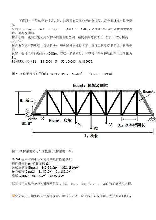
下面以一个简单桁架桥梁为例，以展示有限元分析的全过程。

背景素材选自位于密执安的"Old North Park Bridge" (1904 - 1988)，见图3-22。

该桁架桥由型钢组成，顶梁及侧梁，桥身弦杆，底梁分别采用3种不同型号的型钢，结构参数见表3-6。

桥长L=32m,桥高H=5.5m。

桥身由8段桁架组成，每段长4m。

该桥梁可以通行卡车，若这里仅考虑卡车位于桥梁中间位置，假设卡车的质量为4000kg，若取一半的模型，可以将卡车对桥梁的作用力简化为P1，P2和P3，其中P1= P3=5000 N, P2=10000N，见图3-23。

图3-22位于密执安的"Old North Park Bridge" (1904 - 1988)图3-23桥梁的简化平面模型(取桥梁的一半)表3-6桥梁结构中各种构件的几何性能参数构件惯性矩m4横截面积m2顶梁及侧梁(Beam1) 643.8310m-´322.1910m-´桥身弦梁(Beam2) 61.8710-´31.18510-´底梁(Beam3) 68.4710-´33.03110-´解答以下为基于ANSYS图形界面(Graphic User Interface , GUI)的菜单操作流程。

安全提示：如果聊天中有涉及财产的操作，请一定先核实好友身份。

发送验证问题或点击举报天意11:36:47(1)进入ANSYS（设定工作目录和工作文件）程序→ANSYS →ANSYS Interactive →Working directory（设置工作目录）→Initial jobname（设置工作文件名）:TrussBridge →Run →OK(2)设置计算类型ANSYS Main Menu：Preferences…→Structural →OK(3)定义单元类型hhQÆRRN«•QQoomm QM•9NN•}ANSYS Main Menu：Preprocessor →Element Type →Add/Edit/Delete... →Add…→Beam : 2delastic 3 →OK（返回到Element Types窗口）→Close(4)定义实常数以确定梁单元的截面参数ANSYS Main Menu: Preprocessor →Real Constants…→Add/Edit/Delete →Add…→select Type 1Beam 3 →OK →input Real Constants Set No. : 1 , AREA: 2.1 9E-3，Izz: 3.83e-6(1号实常数用于顶梁和侧梁) →Apply →input Real Constants Set No. : 2 , AREA: 1.18 5E-3，Izz: 1.87E-6 (2号实常数用于弦杆)→Apply →input Real Constants Set No. : 3, AREA: 3.031E-3，Izz: 8.47E-6 (3号实常数用于底梁) →OK(back to Real Constants window) →Close (the Real Constants win dow)(5)定义材料参数ANSYS Main Menu: Preprocessor →Material Props →Material Model s →Structural →Linear→Elastic →Isotropic →input EX: 2.1e11, PRXY: 0.3(定义泊松比及弹性模量) →OK →Density (定义材料密度) →input DENS: 7800, →OK →Close（关闭材料定义窗口）(6)构造桁架桥模型生成桥体几何模型ANSYS Main Menu：Preprocessor →Modeling →Create →Keypoints →In Active CS →NPTKeypoint number：1，X，Y，Z Location in active CS：0，0 →Apply →同样输入其余15个特征点坐标（最左端为起始点，坐标分别为(4,0), (8,0), (12,0), (16,0), (20,0), (24,0), (28,0), (32,0), (4,5 .5), (8,5.5),(12,5.5), (16.5.5), (20,5.5), (24,5.5), (28,5.5)）→Lines →Lines →Straight Line →依次分别连接特征点→OK网格划分ANSYS Main Menu: Preprocessor →Meshing →Mesh Attributes →P icked Lines →选择桥顶梁及侧梁→OK →select REAL: 1, TYPE: 1 →Apply →选择桥体弦杆→OK →select REAL: 2,TYPE: 1 →Apply →选择桥底梁→OK →select REAL: 3, TYPE:1 →OK →ANSYS Main Menu：Preprocessor →Meshing →MeshTool →位于Size Controls下的Lines：Set →Element Size on Picked→Pick all →Apply →NDIV：1 →OK →Mesh →Lines →Pick all →OK (划分网格)(7)模型加约束ANSYS Main Menu: Solution →Define Loads →Apply →Structural →Displacement →OnNodes →选取桥身左端节点→OK →select Lab2: All DOF(施加全部约束) →Apply →选取桥身右端节点→OK →select Lab2: UY(施加Y方向约束) →OK(8)施加载荷ANSYS Main Menu: Solution →Define Loads →Apply →Structural →Force/Moment →OnKeypoints →选取底梁上卡车两侧关键点（X坐标为12及20）→OK →select Lab: FY，Value: -5000→Apply →选取底梁上卡车中部关键点（X坐标为16）→OK →select Lab: FY，Value: -10000 →OK→ANSYS Utility Menu：→Select →Everything(9)计算分析ANSYS Main Menu：Solution →Solve →Current LS →OK(10)结果显示ANSYS Main Menu：General Postproc →Plot Results →Deformed shape →Def shape only →OK（返回到Plot Results）→Contour Plot →Nodal Solu →DOF Solution, Y-Component of D isplacement→OK（显示Y方向位移UY）(见图3-24(a))定义线性单元I节点的轴力ANSYS Main Menu →General Postproc →Element Table →Define Table →Add →Lab:[bar_I], By sequence num: [SMISC,1] →OK →Close定义线性单元J节点的轴力ANSYS Main Menu →General Postproc →Element Table →Define Table →Add →Lab:[bar_J], By sequence num: [SMISC,1] →OK →Close画出线性单元的受力图(见图3-24(b))ANSYS Main Menu →General Postproc →Plot Results →Contour Plot →Line Elem Res →LabI: [ bar_I], LabJ: [ bar_J], Fact: [1] →OK(11)退出系统ANSYS Utility Menu：File →Exit →Save Everything →OK(a)桥梁中部最大挠度值为0.003 374m (b)桥梁中部轴力最大值为25 380N图3.24桁架桥挠度UY以及单元轴力计算结果!%%%%% [ANSYS算例]3.4.2(2) %%%%% begin %%%%%%!------注：命令流中的符号$，可将多行命令流写成一行------/prep7 !进入前处理/PLOPTS,DATE,0 !设置不显示日期和时间!=====设置单元和材料ET,1,BEAM3 !定义单元类型R,1,2.19E-3,3.83e-6, , , , , !定义1号实常数用于顶梁侧梁R,2,1.185E-3,1.87e-6,0,0,0,0, !定义2号实常数用于弦杆R,3,3.031E-3,8.47E-6,0,0,0,0, !定义3号实常数用于底梁MP,EX,1,2.1E11 !定义材料弹性模量MP,PRXY,1,0.30 !定义材料泊松比MP,DENS,1,,7800 !定义材料密度!-----定义几何关键点K,1,0,0,, $ K,2,4,0,, $ K,3,8,0,, $K,4,12,0,, $K,5,16,0,, $K,6,20,0,, $K,7,24,0,, $K,8,28,0,, $K,9,32,0,, $K,10,4,5.5,,$K,11,8,5.5,, $K,12,12,5.5,, $K,13,16,5.5,, $K,14,20,5.5,, $K,15,24,5.5, , $K,16,28,5.5,,!-----通过几何点生成桥底梁的线L,1,2 $L,2,3 $L,3,4 $L,4,5 $L,5,6 $L,6,7 $L,7,8 $L,8,9!------生成桥顶梁和侧梁的线L,9,16 $L,15,16 $L,14,15 $L,13,14 $L,12,13 $L,11,12 $L,10,11 $L,1,10!------生成桥身弦杆的线L,2,10 $L,3,10 $L,3,11 $L,4,11 $L,4,12 $L,4,13 $L,5,13 $L,6,13 $L,6, 14 $L,6,15 $L,7,15 $L,7,16 $L,8,16!------选择桥顶梁和侧梁指定单元属性LSEL,S,,,9,16,1,LATT,1,1,1,,,,hhQÆRRN«•QQoomm QM•9NN•}!-----选择桥身弦杆指定单元属性LSEL,S,,,17,29,1,LATT,1,2,1,,,,!-----选择桥底梁指定单元属性LSEL,S,,,1,8,1,LATT,1,3,1,,,,!------划分网格AllSEL,all !再恢复选择所有对象LESIZE,all,,,1,,,,,1 !对所有对象进行单元划分前的分段设置LMESH,all !对所有几何线进行单元划分!=====在求解模块中，施加位移约束、外力，进行求解/soluNSEL,S,LOC,X,0 !根据几何位置选择节点D,all,,,,,,ALL,,,,, !对所选择的节点施加位移约束AllSEL,all !再恢复选择所有对象NSEL,S,LOC,X,32 !根据几何位置选择节点D,all,,,,,,,UY,,,, !对所选择的节点施加位移约束ALLSEL,all !再恢复选择所有对象!------基于几何关键点施加载荷FK,4,FY,-5000 $FK,6,FY,-5000 $FK,5,FY,-10000/replot !重画图形Allsel,all !选择所有信息(包括所有节点、单元和载荷等)solve !求解!=====进入一般的后处理模块/post1 !后处理PLNSOL, U,Y, 0,1.0 !显示Y方向位移PLNSOL, U,X, 0,1.0 !显示X方向位移!------显示线单元轴力------ETABLE,bar_I,SMISC, 1ETABLE,bar_J,SMISC, 1PLLS,BAR_I,BAR_J,0.5,1 !画出轴力图finish !结束你参考这个例题试一下。

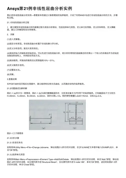
Ansys第21例⾮线性屈曲分析实例第21例⾮线性屈曲分析实例—悬臂梁本例通过计算悬臂梁的临界载荷，介绍了利⽤ANSYS进⾏⾮线性屈曲分析的⽅法、步骤和过程。

21.1⾮线性屈曲分析过程1．建⽴模型⾮线性屈曲分析的建模过程与其他分析相似，包括选择单元类型、定义单元实常数、定义材料特性、定义横截⾯、建⽴⼏何模型和划分⽹格等。

2．求解(1)进⼊求解器。

(2)指定分析类型。

⾮线性屈曲分析属于⾮线性静⼒学分析。

(3)定义分析选项。

激活⼤变形效应。

(4)施加初始⼏何缺陷或初始扰动。

可以先进⾏线性屈曲分析，将分析所得到的屈曲模态形状乘以⼀个较⼩的系数后作为初始扰动施加到结构上，本例即采⽤该⽅法。

(5)施加载荷。

所施加的载荷应⽐预测值⾼10%⼀21%。

(6)定义载荷步选项。

(7)设置弧长法。

(8)求解。

3.查看结果在POST26时间历程后处理器中，建⽴载荷和位移关系曲线，从⽽确定结构的临界载荷。

21.2问题描述及解析解图21-1 (a)所⽰为⼀悬臂梁，图21-1 (b)为梁的横横截⾯形状，分析其在集中⼒P作⽤下的临界载荷。

已知截⾯各尺⼨分别为H=50mm、h=43mm、B=35mm、b=32mm，梁的长度L=1m。

钢的弹性模量E=2xl011N/m2，泊松⽐p=0.3。

图21-1⼯⼦悬臂梁21.3分析步骤21.3.1改变任务名拾取菜单Utility Menu→File→Change Jobname，弹出如图21-2所⽰的对话框，在“[/FJLNAM]”⽂本框中输⼊EXAMPLE21，单击“OK”按钮。

21.3.2选择单元类型拾取菜单Main Menu→Preprocessor→Element Type→Add/Edit/Delete，弹出如图21-3所⽰的对话框，单击“Add.”按钮，弹出如图21-4所⽰的对话框，在左侧列表中选“Structural Beam”，在右侧列表中选“3 node 189”，单击“OK”按钮，返回到如图21-3所⽰的对话框，单击“Close”按钮。

屈曲分析实例：桁架结构屈曲分析框架的端部固定，横截面为边长为150mm的正三角形，框架总长15m，分成15小节，每小节长1m；已知所有杆件为空心圆管，内半径4mm，外半径5mm，所有接头均为完全焊接；材料弹性模量1.5e11pa，泊松比0.35；求该结构顶部三角顶点受均匀集中载荷作用时的屈曲临界载荷。

1.定义单元类型和材料属性Beam 3D 2node 188EX 1.5e11 PRXY 0.352.定义杆件材料性质Main Menu>Preprocessor>Sections>Beam>Common Section3.建模三角形Main Menu>Preprocessor>Modeling>Create>Areas>Polygon>Triangle拉伸三角形面MainMenu>Preprocessor>Modeling>Operate>Extrude>Areas>A long Normal在DIST后面输入1删除多余体和多余面，Delete>Volumes Only or Areas Only指定单元划分尺寸Main Menu>Preprocessor>Meshing>Meshtool 所有三角形边框分成3，3条棱边分成20复制线和单元划分MainMenu>Preprocessor>Modeling>Copy>Lines选择L4,L5,L6,L7,L8,L9ITME Number of copies 输入15DZ Z-offset in active CS 输入1合并关键点和线Main Menu>Preprocessor>Numbering Ctrls>Merge Items在Label后面的下拉列表中选择Keypoint压缩编号Main Menu>Preprocessor>NumberingCtrls>Compress Numbers在Label后面的下拉列表中选择All4.获得静力解Main Menu>Solution>Unabridged>Analysis Type>New Analysis———Static Main Menu>Solution>Unabridged>Analysis Type>Sol'n Controls，勾上Calcutate prestress effects定义边界条件在三角框架端部的3个节点施加全约束在三角框架顶部的3个节点输入力FZ=-1求解Main Menu>Solution>Solve >Current LS退出求解 Main Menu>Finish5.获得特征值屈曲解Main Menu>Solution>Unabridged>Analysis Type>New Analysis———Eigen BuckingMain Menu>Solution>Unabridged>Analysis Options，在NMode No.of modes to extract输入10求解Main Menu>Solution>Solve >Current LS退出求解 Main Menu>Finish6.扩展解Main Menu>Solution>Unabridged>AnalysisType>ExpansionPass，勾上[EXPASS] Expansion Pass设定扩展解Main Menu>Solution >Load Step Opts>ExpansionPass>Single Expand>Expand Modes求解Main Menu>Solution>Solve >Current LS退出求解 Main Menu>Finish7.后处理读入第七阶屈曲模态 Main Menu>General Postproc>Read Results>By Pick 显示七阶屈曲模态Main Menu>General Postproc>Read Results>Plot Results>Deformed+Shape重复上述步骤，可以得到任意阶屈曲模态。

一个屈曲分析实例一、问题和条件：钢闸门断面为工字钢，具体尺寸如下，试作屈曲分析：弹性模量E＝200GPa泊松比μ＝0.3集中力F=1N（单位力）二、进入ANSYS界面单击开始→程序→ansys10.0→configure ANSYS product然后在File Management中定义Working Directory（工作路径）如：class 定义Job Name（工作文件名）。

如：file。

如图所示。

然后，点击run。

三、定义单元及材料1新建单元类型运行主菜单Preprocessor→Element Type→Add/Edit/Delete(新建/编辑/删除单元类型)命令，接着在对话框中单击“Add”按钮新建单元类型。

2定义单元类型因为beam188单元适合于分析柔性梁结构，支持弹性，蠕变和塑性模型的计算。

先选择单元为beam，接着选择3D2node188，然后单击“OK”按钮确定，完成单元类型的选择。

3关闭单元类型对话框回到单元类型对话框，已经新建了beam单元，单击对话框中“Close”按钮关闭对话框。

4定义截面形状及参数运行主菜单Preprocessor→Sections→Beam→Common sections命令，接着在对话框中sub-type中选择“工”字钢断面，在下面的尺寸中分别填入：W1=0.2,W2=0.2,W3=0.4,t1=0.01,t2=0.01,t3=0.01,点击OK结束。

5设置材料属性运行主菜单Preprocessor→Material props→Material Models(材料属性)命令。

选择材料属性命令后，系统会显示材料属性设置对话框。

6设置杨氏弹性模量与泊松比在材料属性设置对话框右侧依次选择Structural→Linear→Elastic→Isotropic。

完成选择命令后，接着在对话框中EX杨氏弹性模量输入2e11，PPXY泊松比输入0.3。

三角桁架受力分析1 问题描述图1所示为一三角析架受力简图。

图中各杆件通过铰链连接，杆件材料参数及几何参数见表1和表2，析架受集中力F1=5000N, F2=3000N 的作用，求析架各点位移及反作用力。

图1 三角桁架受力分析简图表1 杆件材料参数表2 杆件几何参数2 问题分析该问题属于析架结构分析问题。

对于一般的析架结构，可通过选择杆单元，并将析架中各杆件的几何信息以杆单元实常数的形式体现出来，从而将分析模型简化为平面模型。

在本例分析过程中选择LINK l 杆单元进行分析求解。

3 求解步骤3.1 前处理（建立模型及网格划分） 1.定义单元类型及输入实常量选择Structural Link 2D spar 1单元，步骤如下：选择Main Menu|Preprocessor|Element Type|Add Edit/Delete 命令，出现Element Types 对话框，单击Add 按钮，出现Library of Element Types 对话框。

在Library of Element Types 列表框中选择Structural Link 2D spar 1，在Element type reference number 文本框中输入1，单击OK 按钮关闭该对话框。

如图2所示。

E 1/Pa E 2/Pa E 3/Pa ν1 ν2 ν3 2.2E11 6.8E102.0E110.30.260.26L1/m L 1/m L 1/m A 1/m 2 A 2/m 2 A 3/m 2 0.4 0.50.36E-49E-44E-4图2 单元类型的选择输入三杆的实常量（横截面积），步骤如下：选择Main Menu|Preprocessor|Real Constants|Add/Edit/Delete命令，出现Real Constants 对话框，单击Add按钮，出现Element Type for Real Constants对话框，单击OK按钮，出现Real Constant Set Number 1, for LINK1对话框，在Real Constant Set No.文本框中输入1，在Cross-sectional area文本框中输入6E-4，在Initial strain文本框中输入0。

ansys屈曲（Ansys buckling）03 string stability calculation (ANSYS)This example will discuss the eigenvalue instability and nonlinear instability of the string with prestressed stressKnowledge points:(a) prestressed(b) stable eigenvalues(c) consideration of the stability of eigenvalues of other internal forces(d) add initial defect(e) arc n(f) nonlinear analysis and convergence(g) relationship of load displacement(1) set the Parameters of analysis. In the top menu of ANSYS, parameter-> Scalar Parameters, input in the pop-up Scalar Parameters window, FORCE = 100, OFFSET = 0.1.(2) establish a model. In this example, we will contact two new units, three-dimensional Beam unit Beam 4 and 3d cable unit Link 10. The Beam 4 unit is simpler than the Beam 188 unit introduced before, and is also a useful unit for the common rectangularelastic cross section. Link 10 is the space cable unit provided by ANSYS. The user can control the unit only under pressure or can only be pulled. By default, the unit can only be pulled.(3) select Beam 4 units and Link 10 units in the ANSYS main menu Preprocessor - > Element type - > Add/Edit/Delete(4) both Beam 4 and Link 10 can use real parameters to set the section properties. First, the section of the Beam 4 unit is set. The cross section we want to build is a rectangular section of 0.1 m by 0.12 m. If the Beam 4 unit does not specify the direction of the main axis of the section, the Y-axis of the partial coordinate system of the section will be parallel to the x-y plane of the whole coordinate system. In the ANSYS main menu Preprocessor - > Real Constants - > Add/Edit/Delete, select Add, the associated unit type of the specified Real parameter is Beam 4 unit, and the input section parameter is AREA: 0.1 * 0.12, IZZ: 0.12 * 0.1 * * 3/12, IYY: 0.1 * 0.12 * 3/12, TKZ: 0.12, TKY: 0.1, as shown in the figure below(5) continue to add the second real parameter type, and specify that the second real parameter is associated with the Link 10 unit. The sectional area of the Link 10 unit is 4 x 10-6m2, and the initial strain is 2 x 10-3. The initial strain is the strain of strain.(6) the material properties are set below. In this example, all materials are set as steel for simplicity. Add Material properties to the ANSYS main menu Preprocessor - > Material Props - > Material Models. In the Material window, select the Structural - > Linear - > Elastic - > Isotropic, input Elasticmodulus 2 x 109 and poisson ratio 0.27, also can input the Density of the Material, select the Structural - > Density in the Material window, and the input Density is 7800.(7) the geometric model is established. In this example, we still construct geometric models strictly according to the points, lines, planes and body topologies that are required by the modeling process of ANSYS.(8) the key points are established In the ANSYS main menu Preprocessor - > Modeling - > Create - > Keypoints - > In Active CS(9) connect the key points below and connect the following key points in the ANSYS main menu Preprocessor - > Modeling - > create-> Lines - > Straight LineGet the string model(10) to divide the grid by geometry. In the ANSYS main menu Preprocessor - > meshing-> Mesh Attributes - >, line 1, select 1 ~ 6 straight line, setting its unit type, material type and real parameter are all 1. Select the line 7-14, the material type is 1, the unit type and the real parameter are both 2.(11) control the size of the grid. For the analysis, in the middle of the column is the key of the research, the mesh so we want to have to close some, in the ANSYS Preprocessor main menu - > Meshing - > Size Cntrls - > Lines - > Picked Lines, select 1 ~ 6 straight Lines, set the maximum Length of grid unit (Element Edge Length) of 0.3. For the surrounding prestressedcables,Since Link 10 is a relatively complex nonlinear unit, it is easy to solve the difficult convergence problem when solving the problem. Therefore, we divide the prestressed cable into one unit. Select the line 7 ~ 14, and set the number of grid segments as 1.(12) in the ANSYS main menu Preprocessor - > meshing-> Mesh - > Lines, select all the Lines and divide the grid(13) at the top of ANSYS, the menu plotctrls-> Style -- > Size and shape, set Display of element as On. Get the unit shape as shown in the figure:(14) the boundary condition and load are added under the model. Main menu first into the ANSYS Solution - > Define Loads - > Apply - > Structural - > below - > On Keypoints, selected key point 3, constraint three horizontal movement dof UX, UY, offers and rotational degree of freedom ROTZ, select the point 2, two translational degree of freedom UX and UY constraints.(15) enter the ANSYS main menu Solution - > Define Loads - > Apply - > struck-> Force/Moment - > One Keypoints, select key point 2, load direction of FZ and size - Force(16) to conduct a Static Analysis, Solution main menu - > into ANSYS Analysis Type - > New Analysis, set for the Static Analysis of types, into the Solution - > Analysis Type - > Sol 'n Controls, set for small deformation Analysis and consider prestressed, close the automatic time step control steps andset Analysis child (Substeps) to 1(17) for a Solution operation, enter the ANSYS main menu Solution - > Solve - > Current LS.(18) the eigenvalue buckling of the model is solved. Solution main menu - > into ANSYS Analysis Type - > New Analysis, set Analysis of Type Eigen Buckling, Solution main menu - > into ANSYS Analysis Type - > Analysis Options, set the Solution of the first-order stable load.(19) to Solve the operation again, enter the ANSYS main menu Solution - > Solve - > Current LS.(20) into the post-processing operation at this moment, the main menu into ANSYS General Postproc - > Read the results - > the Last Set, Read in the Last step as a result, the main menu select ANSYS General Postproc - > Plot results - > Deformed Shape, they can get form of instability of the structure and the corresponding buckling load magnification, which is 118.602, as shown.(21) enter the Parameters - > Get scalar data at the top of ANSYS, select Results data in Get scalar data, and select Model Results (modal result) in the result, as shown in the figure. Click OK to go to the next window Get Model Results, and select the variable that will store the modal result in the name Freq1. Modal is the first order mode.(22) from the top window of the ANSYS window, the first-order frequency is 118.6021, as shown in the figure(23) the above process is the general process of analyzing eigenvalue instability. However, ANSYS has a defect in the process of analyzing eigenvalues instability. As is known to all, the so-called eigenvalue buckling calculation is to use the structure stiffness matrix minus the geometric stiffness of the structure under load multiplied by a coefficient, when the total stiffness matrix singularity is buckling eigenvalues. ANSYS in dealing with a load caused by stiffness matrix cannot differentiate between we need analysis of the external force load (in this case is top concentration) and don't need the structure of the internal force (for example, the calculation of prestressed) contribution to the geometric stiffness matrix. Therefore, it is incorrect to get the eigenvalue yield of 118602N (equal to the initial value of the initial value of 100 x eigenvalue instability of 118.602). Therefore, the problem must be solved through the following iterative calculation.(24) the basic idea of iterative calculation is to adjust the external load on the structure and to solve the eigenvalue instability magnification of the new load according to the magnification of the load.Repeat the above operation until the magnification of the eigenvalue instability is basically equal to 1. The external load added to the structure is the real eigenvalue instability load. And it doesn't contradict the internal forces. The command flow for iterative computing is as follows:! Set the maximum number of iterations 100 times* to DO, I, 1100,FINISH/ SOLU! Apply new load to the structureFk1 - FK, 2, FZ - FORCE! Static analysisANTYPE, 0! Set time1 TIME,AUTOTS, 0NSUBST, 1,,, 1SSTIF, ONSOLVEFINISH! The eigenvalue instability analysis is carried out / SOLUANTYPE, BUCKLE! Buckling analysisBUCOPT, LANB, 1! Use Block Lanczos solution method, extract 1 modeMXPAND, 1! Expand 1 mode shapePSTRES, ON! The INCLUDE PRESTRESS EFFECTSSOLVEFINISH! The first order frequency of the current eigenvalue instability (magnification)* GET FREQ1, MODE, 1, FREQ* the IF, ABS (FREQ1-1), LT, 0.01, THEN! If the frequency error is less than 1%, exit the loop* the EXIT* ENDIFThe FORCE = FORCE * FREQ1! Otherwise, the load times the new magnification is calculated again* ENDDO(25) after repeating the above process, the structure of real eigenvalue buckling load of 198174 n, visible if does not exclude the prestressed internal force of the influence of the geometric stiffness matrix, calculated the eigenvalue buckling load (118602 n) are much smaller.(26) finally, we have a nonlinear buckling analysis. The buckling load calculated by eigenvalue instability is actually the upper limit solution for ideal material. Due to various initial defects or nonlinear effects of materials, the instability load of the actual structure is usually smaller than that of the eigenvalue. Therefore, nonlinear instability analysis is necessary. In nonlinear instability analysis, initial defects need to be introduced. There are many ways to choose the initial defect, and it is more commonly used to add the eigenvalue instability shape of the structure as the most unfavorable initial defect to the structure. The UPGEOM command is provided in ANSYS to facilitate the implementation of the above process, as described below(27), first of all, we need to get the largest eigenvalue buckling mode of the structure deformation is how much, the first main menu in the ANSYS General Postpro Results - > - > List are Sorted Listing - > Sort Nodes, choose the Results of the total displacement (USUM), the maximal displacement of all Nodes.(28) next, select Parameters - > Get Scalar Data in the top menu of ANSYS and select Results Data - > Other operations in Get Scalar Data(29) in the Get Data from Other POST1 Operations window, select the Data from the sorting result that you just did. The required data is the maximum of the sorted order, which is placed in the DMAX variable.(30) DMAX = 1 can be seen from the Scalar Parameter window(31) use the UPGEOM command to adjust the shape of the structure and apply the initial defect. Select Preprocessor - > Modeling - > Update Geom in the ANSYS main menu. UPGEOM will read the structure from the result file and adjust the geometry of the structure. We set the magnification multiple as OFFSET/DMAX, i.e. the maximum initial defect we need is OFFSET = 0.1, and the maximum deformation in the result file is DMAX, so the magnification ratio is OFFSET/DMAX. Finally, the result of the specified eigenvalue instability analysis is called Case03. RST.(32) after the geometry of the structure has been updated, the nonlinear solution can be performed. We know that the load of the eigenvalue instability of the structure is 198174N, and the maximum load of the structure is the loss of the stability load of the characteristic value of three times, which is the input field in the top of the ANSYS window. The load loading structure is constructed, and the analysis type is set to static analysis.(33) in the end, we have to set the solution method in the solver control.This will automatically track the failure path. Enter the ANSYS main menu Solution - > Analysis Type - > Analysis Options. First,set the Analysis Type in the basic option to analyze the large displacement, and consider the prestress. Set the analysis substeps for 20 steps and output the results per step.(34) select the Advanced NL page in the Solution Controls window, and click on the arc-length Method, which USES the default values for the arc-length Method.Main menu (35) into ANSYS Solution - > Solve - > Current LS, began to calculate the Current problem, because the problem is that we come into contact with the first nonlinear problem, it is necessary to introduce the meaning of the output in ANSYS nonlinear calculation window. Nonlinear computing as we know, there is a convergence problem, in this example, the ANSYS output in the reprocessing window four computing intermediate variables: 2 norm of unbalanced force (F L2), unbalanced force closed then poor (F CRIT), 2 norm of unbalanced moment of L2 (M) and the unbalanced moment then sent CRIT (M). The horizontal axis in the window is the time (calculation process), and the ordinate is the corresponding value. In the case of force, if the two norm of the unbalanced force (F L2) is higher than the unbalance force, the F CRIT indicates that there is no convergence, and the calculation is to be continued. If (F L2) is less than (F CRIT), the two curves of (F L2) and (F CRIT) in the graph intersect, indicating that the step calculation has been convergent and the next load step can be calculated. In this case, the case of convergence is still good, and the general iteration converges once or twice.(36) after the calculation has been completed, the post-stroke processor enters ANSYS, selects TimeHist Postpro, and clicksthe variable button in the toolbar in Time History Variables to select add node Z direction deformation, as shown in the figure. Select node 2.(37) in the Time History Variables window set for UZ_2 X coordinates, Time to light up as Y-axis, click on the plot button on the toolbar, you can get the relative load as shown - vertex deformation curve.In General Postproc, the General Postproc - > Read Results - > By Time/Freq was selected, and the display Time was 0.2 (i.e. the maximum load equivalent to 1/5), and the General Postproc - > Plot Results - > Deformed Shape of ANSYS main menu was selected. Draw the current deformation of the structure as shown. Gradually increase the result Time, showing the deformation of Time = 0.4 and 0.6.。