UG7.0高级仿真

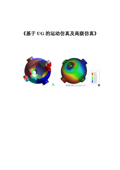
《基于UG的运动仿真及高级仿真》项目一：机构运动仿真项目要求：熟悉UG机构运动仿真模块的内容，掌握运动仿真的一般流程和方法，并根据分析输出结果对机构进行优化。

任务一：熟悉掌握运动仿真基础知识运动分析模块（Scenario for motion）是UG/CAE模块中的主要部分，用于建立运动机构模型，分析其运动规律。

通过UG/Modeling的功能建立一个三维实体模型，利用UG/Motion的功能给三维实体模型的各个部件赋予一定的运动学特性，再在各个部件之间设立一定的连接关系既可建立一个运动仿真模型。

UG/Motion模块可以进行机构的干涉分析，跟踪零件的运动轨迹，分析机构中零件的速度、加速度、作用力、反作用力和力矩等。

运动分析模块的分析结果可以指导修改零件的结构设计（加长或缩短构件的力臂长度、修改凸轮型线，调整齿轮比等）或调整零件的材料（减轻或加重或增加硬度等）。

设计的更改可以反映在装配主模型的复制品分析方案中，再重新分析，一旦确定优化的设计方案，设计更改就可反映在装配主模型中。

一、运动方案创建步骤1．创建连杆（Links）；2．创建两个连杆间的运动副（Joints）3．定义运动驱动（Motion Driver）◆无运动驱动（none）：构件只受重力作用◆运动函数：用数学函数定义运动方式◆恒定驱动：恒定的速度和加速度◆简谐运动驱动：振幅、频率和相位角◆关节运动驱动：步长和步数二、创建连杆创建连杆对话框将显示连杆默认的名字，格式为L001、L002 (00)质量属性选项：质量特性可以用来计算结构中的反作用力。

当结构中的连杆没有质量特性时，不能进行动力学分析和反作用力的静力学分析。

根据连杆中的实体，可以按默认设置自动计算质量特性，在大多数情况下，这些默认计算值可以生成精确的运动分析结果。

但在某些特殊情况下，用户必须人工输入这些质量特性。

固定连杆：人工输入质量属性，需要指定质量、惯性矩、初始移动速度和初始转动速度。

高级仿真高级仿真 (1)NX Nastran structural analysis and solution types (2)NX Nastran thermal analysis and solution types (4)线性静态分析 (4)Supported linear static analysis types (4)Using materials for a linear static analysis (5)Defining boundary conditions for a linear static analysis (5)Using the iterative solver (5)模态分析 (6)Supported modal analysis types (6)Using materials for a modal analysis (7)Defining boundary conditions for a modal analysis (7)Setting modal solution attributes (7)Reviewing modal analysis results (8)如何判断模态的频率 (8)线性曲屈分析 (9)Buckling analysis introduction (9)Linear buckling assumptions (9)Supported buckling analysis types (10)Using materials for a buckling analysis (10)Defining boundary conditions for a buckling analysis (10)Reviewing buckling analysis results (10)Nonlinear static analysis introduction (11)Supported nonlinear solution types (11)Whether to use a nonlinear solution (12)Using elements for solution type NLSTATIC 106 (13)Using elements for solution type ADVNL 601, 106 (13)Using materials for solution types NLSTATIC 106 and ADVNL 601, 106 (14)Entering stress/strain data for solution types NLSTATIC 106 and ADVNL 601, 106 (14)Defining boundary conditions for solution types NLSTATIC 106 and ADVNL 601, 106 (16)NLSTATIC 106的求解设置 (16)ADVNL 601, 106的求解设置 (17)响应仿真 (17)仿真步骤 (17)Special boundary conditions (19)Solution attributes for Response Simulation (21)FRF and Transmissibility (21)Analysis events (21)Excitation loads (22)Function tools for Response Simulation utility (23)Sensors (23)Strain gages (23)产生整个模型在极值点处的响应 (24)柔体分析 (25)Flexible bodies workflow (25)Advanced Simulation steps (25)Motion Simulation steps (26)Connecting the flexible body FEM to the mechanism (26)Defining connection and load degrees of freedom (26)NX Nastran structural analysis and solution typesNX Nastran thermal analysis and solution types线性静态分析Supported linear static analysis typesIn Advanced Simulation, you can choose from the following linear static analysis types when you create a structural solution.Using materials for a linear static analysis Material types that can be used in a linear static analysis include:•Isotropic•Orthotropic•Anisotropic•LaminateDefining boundary conditions for a linear static analysisBoundary conditions for linear static analysis can be geometry-based or finite element-based. Examples include:•Point and edge forces•Face loads•Temperature loads•Displacement constraints•Coupled degrees of freedomUsing the iterative solverYou can turn on the Element Iterative Solver option on the Solution dialog box, or when you are prompted after you start a solve.The iterative solver:•Can be faster, uses less memory, and has fewer disk requirements than the standard sparse matrix solver.•Can be used for a linear static analysis that does not include contact. • Shows the best performance gain with models composed mostly of solid elements.• Is very efficient for models composed mostly of parabolic tetrahedral elements.模态分析Supported modal analysis typesIn Advanced Simulation, you can choose from the following modal analysis types when you create a structural solution: SolverSolution type NX NastranSEMODES 103SEMODES 103 - Response SimulationSEMODES 103 - Superelement SEMODES 103 - Flexible Body MSC NastranSEMODES 103SEMODES 103 - SuperelementUsing materials for a modal analysisMaterial types that can be used in a modal analysis include:•Isotropic•Orthotropic•Anisotropic•FluidDefining boundary conditions for a modal analysisBoundary conditions for modal analysis include constraints and gluing, such as:•Displacement constraints.•Coupled degrees of freedom.•Surface-to-surface gluingSetting modal solution attributesFor a modal analysis, some of the NX Nastran solution attributes include:•Max Job Time•Output Requests•Real Eigenvalue Extraction Data. Identifies the type of solve: Lanczos or Householder.•Lanczos Method or Householder Method. The method specifies the real eigenvalue extraction options for the solution. Eigenvalueextraction options are stored as a solver-specific object. Lanczos is the recommended method for most models; Householder isrecommended for smaller models.The options include frequency range lower and upper limits, and the number of desired modes.•Default TemperatureFor more information, see Solvers and Solutions→Setting Nastran Solution Options in the Advanced Simulation online Help.Reviewing modal analysis resultsNatural frequencies and mode shapes are the primary results for a modal solution.•The results are ordered by frequency, with the lowest natural frequency being the first mode shape, the next highest being the second mode, and so on.•The normal modes represent dynamic states in which the elastic and inertial forces are balanced when no external loads are applied.The magnitude of the mode shapes is arbitrary.•The amplitude of the displacement is not significant, but the relative displacement of the nodes is significant.•Mode shapes help you determine what load locations and directions will excite the structure.如何判断模态的频率The first 6 modes have extremely low frequencies. These are rigid body modes. Mode 7 represents the first flexible mode with a natural frequency of about 133 Hz.线性曲屈分析Buckling analysis introductionBuckling analysis:•Determines buckling loads and buckled mode shapes.o A buckling load is the critical load at which a structure becomes unstable.o A buckled mode shape is the characteristic shape associated with a structure's buckled response.•Identifies the critical load factor, which is the value that can be multiplied by the applied load to cause buckling.Linear buckling assumptionsThe buckling analysis uses linear theory. The following assumptions and limitations apply:•The deflections prior to buckling are small.•The reference equilibrium configuration is the initial geometry of the part.•The response of the structure prior to buckling exhibits a linear relationship between stress and strain.•Post-buckling behavior is not predictedSupported buckling analysis typesIn Advanced Simulation, you can choose from the following buckling analysis types when you create a buckling solution:Using materials for a buckling analysisMaterial types that can be used in a buckling analysis include: •Isotropic•Orthotropic•AnisotropicDefining boundary conditions for a buckling analysisFor a buckling analysis:1.Define constraints. Constrain the model as you would for a linearstatic analysis.2.Apply loads. The load set can contain more than one load type (Force,Pressure), but every load will be scaled by the load factor. Amagnitude of 1 is often used when a single load type will cause the model to buckle.Reviewing buckling analysis resultsFor NX Nastran results, buckling analysis results are listed as: • A set of static analysis results for the buckling loads subcase.• A set of modes for the buckling methods subcase.o Each mode has an eigenvalue (load factor) listed.o The applied load multiplied by the buckling load factor is the load at which the part will buckle.o The first mode has the lowest buckling load factor and is usually the mode of most interest.o If the buckling load factor is below 1, the part has buckled.如果eigenvalue小于1，那么这个模型就已经发生曲屈。

UG有限元⾼级仿真--真正有⽤的资料⾼级仿真⾼级仿真 (1)NX Nastran structural analysis and solution types (2)NX Nastran thermal analysis and solution types (4)线性静态分析 (4)Supported linear static analysis types (4)Using materials for a linear static analysis (5)Defining boundary conditions for a linear static analysis (5)Using the iterative solver (5)模态分析 (6)Supported modal analysis types (6)Using materials for a modal analysis (7)Defining boundary conditions for a modal analysis (7)Setting modal solution attributes (7)Reviewing modal analysis results (8)如何判断模态的频率 (8)线性曲屈分析 (9)Buckling analysis introduction (9)Linear buckling assumptions (9)Supported buckling analysis types (10)Using materials for a buckling analysis (10)Defining boundary conditions for a buckling analysis (10)Reviewing buckling analysis results (10)Nonlinear static analysis introduction (11)Supported nonlinear solution types (11)Whether to use a nonlinear solution (12)Using elements for solution type NLSTATIC 106 (13)Using elements for solution type ADVNL 601, 106 (13)Using materials for solution types NLSTATIC 106 and ADVNL 601, 106 (14)Entering stress/strain data for solution types NLSTATIC 106 and ADVNL 601, 106 (14) Defining boundary conditions for solution types NLSTATIC 106 and ADVNL 601, 106 (16) NLSTATIC 106的求解设置 (16)ADVNL 601, 106的求解设置 (17)响应仿真 (17)仿真步骤 (17)Special boundary conditions (19)Solution attributes for Response Simulation (21)FRF and Transmissibility (21)Analysis events (21)Excitation loads (22)Function tools for Response Simulation utility (23) Sensors (23)Strain gages (23)产⽣整个模型在极值点处的响应 (24)柔体分析 (25)Flexible bodies workflow (25)Advanced Simulation steps (25)Motion Simulation steps (26)Connecting the flexible body FEM to the mechanism (26) Defining connection and load degrees of freedom (26) NX Nastran structural analysis and solution typesNX Nastran thermal analysis and solution types线性静态分析Supported linear static analysis typesIn Advanced Simulation, you can choose from the following linear static analysis types when you create a structural solution.Using materials for a linear static analysis Material types that can be used in a linear static analysis include:IsotropicOrthotropicAnisotropicLaminateDefining boundary conditions for a linear static analysisBoundary conditions for linear static analysis can be geometry-based or finite element-based. Examples include:Point and edge forcesFace loadsTemperature loadsDisplacement constraintsCoupled degrees of freedomUsing the iterative solverYou can turn on the Element Iterative Solver option on the Solution dialog box, or when you are prompted after you start a solve.The iterative solver:Can be faster, uses less memory, and has fewer disk requirements than the standard sparse matrix solver.Can be used for a linear static analysis that does not include contact.Shows the best performance gain with models composed mostly of solid elements.Is very efficient for models composed mostly of parabolic tetrahedral elements.模态分析Supported modal analysis typesIn Advanced Simulation, you can choose from the following modal analysis types when you create a structural solution: SolverSolution typeNX NastranSEMODES 103SEMODES 103 - Response SimulationSEMODES 103 - SuperelementSEMODES 103 - Flexible BodyMSC NastranSEMODES 103SEMODES 103 - SuperelementUsing materials for a modal analysisMaterial types that can be used in a modal analysis include:IsotropicOrthotropicAnisotropicFluidDefining boundary conditions for a modal analysisBoundary conditions for modal analysis include constraints and gluing, such as:Displacement constraints.Coupled degrees of freedom.Surface-to-surface gluingSetting modal solution attributesFor a modal analysis, some of the NX Nastran solution attributes include:Max Job TimeOutput RequestsReal Eigenvalue Extraction Data. Identifies the type of solve: Lanczos or Householder.Lanczos Method or Householder Method. The method specifies the real eigenvalue extraction options for the solution. Eigenvalueextraction options are stored as a solver-specific object. Lanczos is the recommended method for most models; Householder isrecommended for smaller models.The options include frequency range lower and upper limits, and the number of desired modes.Default TemperatureFor more information, see Solvers and Solutions→Setting Nastran Solution Options in the Advanced Simulation online Help. Reviewing modal analysis resultsNatural frequencies and mode shapes are the primary results for a modal solution.The results are ordered by frequency, with the lowest natural frequency being the first mode shape, the next highest being the second mode, and so on.The normal modes represent dynamic states in which the elastic and inertial forces are balanced when no external loads are applied.The magnitude of the mode shapes is arbitrary.The amplitude of the displacement is not significant, but the relative displacement of the nodes is significant.Mode shapes help you determine what load locations and directions will excite the structure.如何判断模态的频率The first 6 modes have extremely low frequencies. These are rigid body modes. Mode 7 represents the first flexible mode with a natural frequency of about 133 Hz.线性曲屈分析Buckling analysis introductionBuckling analysis:Determines buckling loads and buckled mode shapes.o A buckling load is the critical load at which a structure becomes unstable.o A buckled mode shape is the characteristic shape associated with a structure's buckled response.Identifies the critical load factor, which is the value that can be multiplied by the applied load to cause buckling. Linear buckling assumptionsThe buckling analysis uses linear theory. The following assumptions and limitations apply:The deflections prior to buckling are small.The reference equilibrium configuration is the initial geometry of the part.The response of the structure prior to buckling exhibits a linear relationship between stress and strain.Post-buckling behavior is not predictedSupported buckling analysis typesIn Advanced Simulation, you can choose from the following buckling analysis types when you create a buckling solution:Using materials for a buckling analysisMaterial types that can be used in a buckling analysis include: ?IsotropicOrthotropicAnisotropicDefining boundary conditions for a buckling analysisFor a buckling analysis:1.Define constraints. Constrain the model as you would for a linearstatic analysis.2.Apply loads. The load set can contain more than one load type (Force,Pressure), but every load will be scaled by the load factor. Amagnitude of 1 is often used when a single load type will cause the model to buckle.Reviewing buckling analysis resultsFor NX Nastran results, buckling analysis results are listed as: ? A set of static analysis results for the buckling loads subcase.A set of modes for the buckling methods subcase.o Each mode has an eigenvalue (load factor) listed.o The applied load multiplied by the buckling load factor is the load at which the part will buckle.o The first mode has the lowest buckling load factor and is usually the mode of most interest.o If the buckling load factor is below 1, the part has buckled.如果eigenvalue⼩于1，那么这个模型就已经发⽣曲屈。

基于UG的C型钳有限元分析及优化设计谢晓华【摘要】应用UG NX7.0的"高级仿真"模块,建立C型钳的有限元模型.通过解算器NX NASTRAN对有限元模型进行分析求解,得到C型钳在额定载荷时的位移变形和应力分布情况,再根据设计要求对零件参数进行优化,使C型钳的结构既满足设计要求,又达到体积小、成本低的目的.【期刊名称】《机电产品开发与创新》【年(卷),期】2010(023)004【总页数】2页(P111-112)【关键词】UG;有限元;C型钳;优化【作者】谢晓华【作者单位】永州职业技术学院,湖南,永州,425100【正文语种】中文【中图分类】TP391.90 引言C型钳结构简单，生产成本低，可对零件精确定位、快速装卸，自锁夹紧，并可单向、双向和多向夹持零件，广泛应用于机械加工、装配和模具等领域。

C型钳的结构强度对它的夹持力有着直接的影响，采用传统的工程力学计算方法难以准确求出C型钳的应力分布情况,尤其难以精确求解局部应力集中的位置及大小。

在C型钳的研发阶段引入有限元分析技术，先对产品进行参数化建模，再用有限元方法对产品进行静力学分析，并对产品的参数化结构进行优化，可提高产品质量和降低产品成本，为该产品的研发提供了指导意义。

有限元分析的思路是：结构离散→单元分析→整体求解。

有限元分析可分成三个阶段：①建立有限元模型，完成单元网格划分等；②运用有限元解算器对有限元模型进行分析；③采集处理分析结果，使用户能提取计算结果。

1 有限元分析模型准备1.1 建立有限元模型首先在UG NX7.0模块中建立C型钳的三维模型，如图1所示。

C型钳的钳体各部位受力差异较大，是需校核的重要构件，因此主要选择钳体进行有限元分析。

进入“高级仿真” 应用模块，建立钳体的“FEM和仿真”部件文件，选择有限元解算器为“NX NASTRAN”，分析类型为“结构”，解算方案类型为“SESTATEC 101-单约束”，启用迭代求解器，接受系统设置的其它各项值，完成解算方案的设置。

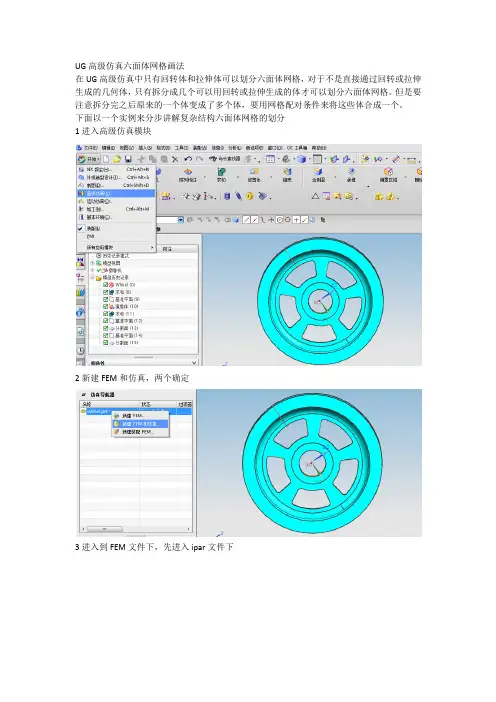
UG高级仿真六面体网格画法
在UG高级仿真中只有回转体和拉伸体可以划分六面体网格，对于不是直接通过回转或拉伸生成的几何体，只有拆分成几个可以用回转或拉伸生成的体才可以划分六面体网格。

但是要注意拆分完之后原来的一个体变成了多个体，要用网格配对条件来将这些体合成一个。

下面以一个实例来分步讲解复杂结构六面体网格的划分
1进入高级仿真模块
2新建FEM和仿真，两个确定
3进入到FEM文件下，先进入ipar文件下
4提升体
6拆分体
将模型拆分成可以用旋转或拉伸生成的多个体，用拆分体命令。

可以选择平面、拉伸或者回转对模型进行拆分。

7检查可扫掠的体
在拆分体命令下有一项是检查可扫掠的体，打开后可查看那些体可以进行花六面体网格。

其中现实绿色的表示可以扫掠，黄色的有可能可以，红色的表示不可以。

8进行网格配对
网格配对的目的是将拆分的体进行合并成原来的一个体，配对类型选择第一项粘连重合。

9划分3D扫掠网格
选择相应的旋转或拉伸平面，划分3D扫掠网格。

10划分完成之后。