83图的矩阵表示

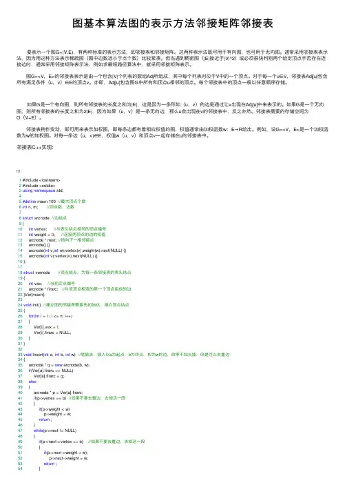
图基本算法图的表⽰⽅法邻接矩阵邻接表 要表⽰⼀个图G=(V,E)，有两种标准的表⽰⽅法，即邻接表和邻接矩阵。

这两种表⽰法既可⽤于有向图，也可⽤于⽆向图。

通常采⽤邻接表表⽰法，因为⽤这种⽅法表⽰稀疏图（图中边数远⼩于点个数）⽐较紧凑。

但当遇到稠密图（|E|接近于|V|^2）或必须很快判别两个给定顶点⼿否存在连接边时，通常采⽤邻接矩阵表⽰法，例如求最短路径算法中，就采⽤邻接矩阵表⽰。

图G=<V，E>的邻接表表⽰是由⼀个包含|V|个列表的数组Adj所组成，其中每个列表对应于V中的⼀个顶点。

对于每⼀个u∈V，邻接表Adj[u]包含所有满⾜条件（u，v）∈E的顶点v。

亦即，Adj[u]包含图G中所有和顶点u相邻的顶点。

每个邻接表中的顶点⼀般以任意顺序存储。

如果G是⼀个有向图，则所有邻接表的长度之和为|E|，这是因为⼀条形如（u，v）的边是通过让v出现在Adj[u]中来表⽰的。

如果G是⼀个⽆向图，则所有邻接表的长度之和为2|E|，因为如果（u，v）是⼀条⽆向边，那么u会出现在v的邻接表中，反之亦然。

邻接表需要的存储空间为O（V+E）。

邻接表稍作变动，即可⽤来表⽰加权图，即每条边都有着相应权值的图，权值通常由加权函数w：E→R给出。

例如，设G=<V，E>是⼀个加权函数为w的加权图。

对每⼀条边（u，v)∈E，权值w（u，v）和顶点v⼀起存储在u的邻接表中。

邻接表C++实现:1 #include <iostream>2 #include <cstdio>3using namespace std;45#define maxn 100 //最⼤顶点个数6int n, m; //顶点数，边数78struct arcnode //边结点9 {10int vertex; //与表头结点相邻的顶点编号11int weight = 0; //连接两顶点的边的权值12 arcnode * next; //指向下⼀相邻接点13 arcnode() {}14 arcnode(int v,int w):vertex(v),weight(w),next(NULL) {}15 arcnode(int v):vertex(v),next(NULL) {}16 };1718struct vernode //顶点结点，为每⼀条邻接表的表头结点19 {20int vex; //当前定点编号21 arcnode * firarc; //与该顶点相连的第⼀个顶点组成的边22 }Ver[maxn];2324void Init() //建⽴图的邻接表需要先初始化，建⽴顶点结点25 {26for(int i = 1; i <= n; i++)27 {28 Ver[i].vex = i;29 Ver[i].firarc = NULL;30 }31 }3233void Insert(int a, int b, int w) //尾插法，插⼊以a为起点，b为终点，权为w的边，效率不如头插，但是可以去重边34 {35 arcnode * q = new arcnode(b, w);36if(Ver[a].firarc == NULL)37 Ver[a].firarc = q;38else39 {40 arcnode * p = Ver[a].firarc;41if(p->vertex == b) //如果不要去重边，去掉这⼀段42 {43if(p->weight < w)44 p->weight = w;45return ;46 }47while(p->next != NULL)48 {49if(p->next->vertex == b) //如果不要去重边，去掉这⼀段50 {51if(p->next->weight < w);52 p->next->weight = w;53return ;54 }55 p = p->next;56 }57 p->next = q;58 }59 }60void Insert2(int a, int b, int w) //头插法，效率更⾼，但不能去重边61 {62 arcnode * q = new arcnode(b, w);63if(Ver[a].firarc == NULL)64 Ver[a].firarc = q;65else66 {67 arcnode * p = Ver[a].firarc;68 q->next = p;69 Ver[a].firarc = q;70 }71 }7273void Insert(int a, int b) //尾插法，插⼊以a为起点，b为终点，⽆权的边，效率不如头插，但是可以去重边74 {75 arcnode * q = new arcnode(b);76if(Ver[a].firarc == NULL)77 Ver[a].firarc = q;78else79 {80 arcnode * p = Ver[a].firarc;81if(p->vertex == b) return; //去重边，如果不要去重边，去掉这⼀句82while(p->next != NULL)83 {84if(p->next->vertex == b) //去重边，如果不要去重边，去掉这⼀句85return;86 p = p->next;87 }88 p->next = q;89 }90 }91void Insert2(int a, int b) //头插法，效率跟⾼，但不能去重边92 {93 arcnode * q = new arcnode(b);94if(Ver[a].firarc == NULL)95 Ver[a].firarc = q;96else97 {98 arcnode * p = Ver[a].firarc;99 q->next = p;100 Ver[a].firarc = q;101 }102 }103void Delete(int a, int b) //删除以a为起点，b为终点的边104 {105 arcnode * p = Ver[a].firarc;106if(p->vertex == b)107 {108 Ver[a].firarc = p->next;109 delete p;110return ;111 }112while(p->next != NULL)113if(p->next->vertex == b)114 {115 p->next = p->next->next;116 delete p->next;117return ;118 }119 }120121void Show() //打印图的邻接表（有权值）122 {123for(int i = 1; i <= n; i++)124 {125 cout << Ver[i].vex;126 arcnode * p = Ver[i].firarc;127while(p != NULL)128 {129 cout << "->(" << p->vertex << "," << p->weight << ")";130 p = p->next;131 }132 cout << "->NULL" << endl;133 }134 }135136void Show2() //打印图的邻接表(⽆权值）137 {138for(int i = 1; i <= n; i++)140 cout << Ver[i].vex;141 arcnode * p = Ver[i].firarc;142while(p != NULL)143 {144 cout << "->" << p->vertex;145 p = p->next;146 }147 cout << "->NULL" << endl;148 }149 }150int main()151 {152int a, b, w;153 cout << "Enter n and m：";154 cin >> n >> m;155 Init();156while(m--)157 {158 cin >> a >> b >> w; //输⼊起点、终点159 Insert(a, b, w); //插⼊操作160 Insert(b, a, w); //如果是⽆向图还需要反向插⼊161 }162 Show();163return0;164 }View Code 邻接表表⽰法也有潜在的不⾜之处，即如果要确定图中边（u,v）是否存在，只能在顶点u邻接表Adj[u]中搜索v，除此之外没有其他更快的办法。

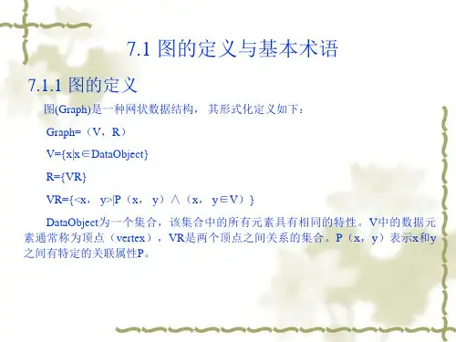
图论基础图的表示与常见算法图论是数学的一个分支，研究的是图这种数学结构。

图由节点（顶点）和边组成，是研究网络、关系、连接等问题的重要工具。

在图论中，图的表示和算法是非常重要的内容，本文将介绍图的表示方法以及一些常见的图算法。

一、图的表示1. 邻接矩阵表示法邻接矩阵是表示图的一种常见方法，适用于稠密图。

对于一个有n 个节点的图，邻接矩阵是一个n×n的矩阵，其中第i行第j列的元素表示节点i到节点j是否有边相连。

如果有边相连，则该元素的值为1或边的权重；如果没有边相连，则该元素的值为0或者无穷大。

邻接矩阵的优点是可以方便地进行边的查找和修改，但缺点是对于稀疏图来说，会浪费大量的空间。

2. 邻接表表示法邻接表是表示图的另一种常见方法，适用于稀疏图。

对于一个有n 个节点的图，邻接表是一个长度为n的数组，数组中的每个元素是一个链表，链表中存储了与该节点相连的其他节点。

邻接表的优点是节省空间，适用于稀疏图，但缺点是查找边的时间复杂度较高。

3. 关联矩阵表示法关联矩阵是表示图的另一种方法，适用于有向图。

对于一个有n个节点和m条边的图，关联矩阵是一个n×m的矩阵，其中第i行第j列的元素表示节点i和边j的关系。

如果节点i是边j的起点，则该元素的值为-1；如果节点i是边j的终点，则该元素的值为1；如果节点i与边j无关，则该元素的值为0。

关联矩阵适用于有向图，可以方便地表示节点和边之间的关系。

二、常见图算法1. 深度优先搜索（Depth First Search，DFS）深度优先搜索是一种用于遍历或搜索图的算法。

从起始节点开始，沿着一条路径一直向下搜索，直到到达叶子节点，然后回溯到上一个节点，继续搜索其他路径。

DFS可以用递归或栈来实现。

2. 广度优先搜索（Breadth First Search，BFS）广度优先搜索是另一种用于遍历或搜索图的算法。

从起始节点开始，先访问起始节点的所有邻居节点，然后再依次访问邻居节点的邻居节点，以此类推。

TI-83+/TI-84 Tutorial: The Basics, Graphing, and Matrices In this tutorial, I will be assuming you have never used a TI graphing calculator before. We will cover what you would need in a basic algebra or precalculus class. Detailed answers/keystrokes for all examples are at the end of each section.If you are following this tutorial on a TI-84 calculator you may have Mathprint installed. Turn Mathrprint off if you want to follow the keystrokes given in the answers. You can turn Mathprint off by going to [MODE] and pressing the [UP ARROW] key until MATHPRINT is highlighted. Use the [RIGHT ARROW] keyso that CLASSIC is highlighted instead and press [ENTER]. Now that Mathprint is turned off, use[2nd][MODE] to go back to the home screen.Table of ContentsI. Basic Layout and Functions (3)Basic Layout – First Look: (3)Navigating and Editing: (5)Section answers: (6)II. Graphing (7)Overview: (7)Example 1: (7)Example 2: (9)Example 3: (9)Section answers: (10)III. Matrices (11)Overview: (11)Entering a Matrix: (11)Arithmetic on a Matrix: (11)Row Reduction on a Matrix : (12)Section answers: (12)IV. Tips and Tricks (14)Degrees and Radians: (14)Fractions and Decimals: (14)Recalling Previous Answers: (14)Section answers: (15)V. Troubleshooting (16)Changing Brightness: (16)Hanging Calculation/Not Responsive: (16)Resetting Memory: (16)Error Screens: (16)VI. - Conclusion (18)I. Basic Layout and FunctionsBasic Layout – First Look:Before you even turn on your calculator, look at how it is organized.The TI-83 can be divided roughly into three sections: Graphing is along the top row, advanced functions and menus is the top middle, and the scientific calculator takes up the bottom half.Above every key you’ll see a secondary function in yellow lettering (blue on a TI-84) or green lettering. To access them, press the [2nd] or [ALPHA] keys first. This is the equivalent of shift on a keyboard.In the bottom half you have basic operations and constants. I’ve marked a few common ones.It is important to note that there is a difference between “negative” and “minus”. Negative has one operand and minus has two operands. For instance, “2 minus 1” versus “negative 2 minus 1”.Turn the calculator on in the lower left-hand corner. (Turn it off again with the [2nd] key.) The screen you see when you first turn on the calculator is called the home screen. The home screen is where most calculations are carried out. Simply type out the operations you want and hit [ENTER]. You can always reach the home screen again from any menu with the [QUIT] function ([2nd][MODE]). And you can always clear the home screen by hitting [CLEAR] twice.Try calculating the following examples on the home screen:1)3-3 = 0 (Basic Arithmetic)2)-9+6(8-5) = 9 (Basic Arithmetic)3)1+(1+.05)14 = 2.979931599 (Exponents)4)log5(48) = 2.405312427 (Logs)5) 6.022E23/1.6E-14 = 3.76375E37 (Scientific Notation)6)4−(1+0.5)7+3= .25 (Basic Arithmetic)Navigating and Editing:To move the cursor around the home screen and any menus, use the arrow keys. Also, as stated before, use [2nd][MODE] to quit back to the home screen whenever you wish.One advantage of a graphing calculator is that you can correct mistakes. Use [CLEAR] to delete a line entirely. [DEL] deletes the character your cursor is on. [INS] changes the cursor to begin inserting what you type rather than overwriting.When you’ve made a mistake on a long calculation, try editing it rather than retyping it entirely. It will save time and help to familiarize yourself with the controls.Section answers:1) [3][-][3][ENTER]2) [(-)][9][+][6][(][8][-][5][)][ENTER]3) [1][+][(][1][+][.][0][5][)][^][1][4][ENTER]4) [LOG][4][8][)][/][LOG][5][)][ENTER]5) [6][.][0][2][2][2nd][,][2][3][/][1][.][6][2nd][,][(-)][1][4][ENTER]or[(][6][.][0][2][2][*][1][0][^][2][3][)][/][(][1][.][6][*][1][0][^][(-)][1][4][ENTER] 6) [(][4][-][(][1][+][.][5][)][)][/][(][7][+][3][)][ENTER]II. GraphingOverview:Everything related to graphing is in the top row of keys. Very quickly, here is a summary of what they do. You won’t be using all these menus equally, and I’ve bolded the most important ones. It will be easier to see how they interact through the examples.●Y= : Enter the equations to graph.●Stat Plot: Set options for plots.●Window: Manually set the window boundaries.●Tblset: Options for the Table.●Zoom: Preset window boundary options.●Format: Options for the appearance of the graphing window.●Trace: Brings up a cursor so you can “trace” a line using the arrow keys.●Calc: Menu with a list of available graphing commands.●Graph: The graphing window itself.●Table: Table of x and y coordinates for each line.It is important to know how to change the boundaries of the graphing window, so that you can view lines that are out of range. [WINDOW] lets you manually set the boundaries, and [ZOOM] has a variety of preset boundaries. (We will do an example in Example 1.)The most useful ZOOM commands are:●Zoom In: Zooms into the blinking cursor when ENTER is pressed.●Zoom Out: Zooms out from the blinking cursor when ENTER is pressed.●ZStandard: Resets the window to [-10,10] [-10,10]Example 1:Let’s experiment with the windowing with some simple graphs. We will graph two linear linesand adjust the window to see where they intersect.1) In the [Y=] menu type 3x+4 into Y1. (The shortcut for ‘x’ is [X,T,Θ,n])2) Type -5x-40 into Y2. (Typing these equations into [Y=] means these will be graphed when [GRAPH] is selected. All equations need to be in y= format.)3) Select ZStandard in the [ZOOM] menu. The two lines should be drawn on the screen4) As you can see, the intersection of the two lines is past the bottom of the screen. We will need to increase Y min in order to see the intersection. Go to the [WINDOW] menu and change Y min from -10 to -20.5) Select [GRAPH]. By changing the window boundary, we can now see the intersection.6) Select [TRACE]. Use this to practice navigating along the lines. Using the arrow keys, UP and DOWN switch you from line to line. LEFT and RIGHT move you along a single line. The x and y coordinates of the cursor will show up along the bottom of the screen. The line the cursor is currently on will show up on the upper left corner of the screen.7) Select ZStandard in the [ZOOM] menu again. As you can see, the window resets to [-10,10] [-10,10].8) Select Zoom Out in the [ZOOM] menu. You should now see a small blinking cursor on the graph. You can move the cursor around with the arrow keys. Press [ENTER] when you’re ready to zoom out, and the graph expand from where the cursor is. You should be able to see the intersection again.9) Select Zoom In from the [ZOOM] menu. Move the cursor as close to the intersection you can and hit [ENTER]. The graph should be zoomed into where the cursor was, near the intersection.This shows you how the [Y=], [WINDOW], [ZOOM], and [GRAPH] menus interact. [Y=] defines what to graph, [ZOOM] and [WINDOW] define the boundaries of the graph, and [GRAPH] is where the actual graph is drawn.Example 2:Let’s carry on from the previous example by actually calculating the intersection of the two lines. Intersect and all other graphing calculations are found in the [CALC] menu.10) Select intersect from the [CALC] menu. You will see three questions in turn in the lower left corner: First Curve?, Second Curve?,and Guess?. Hit [ENTER] to select 3x+4 as the first curve, and [ENTER] again to select -5x-40 as the second curve. (If there are many lines, use the up and down arrow keys as needed to select the correct lines.) Guess means to select a suitable starting point for the calculation. In this example, any starting point will do. After you hit [ENTER] one more time, the point (-5.5,-12.5) should be highlighted. (Any starting point works here because there is only one intersection. If there is more than one intersection, it will find the one closest to your cursor. Use the left and right arrow keys to move the cursor along a line.)Example 3:Another common calculation is to find the minimum or maximum of a function. Because straight lines don’t have minimums or maximums, let’s clear Y1 and Y2 and try a different curve.11) Clear Y1 and Y2. Enter x2+4x-3 into Y1.12) Select ZStandard in the [ZOOM] menu.13) Select minimum from the [CALC] menu. You will again see three questions in turn in the lower left corner: Left Bound?,Right Bound?, and Guess?. The Left Bound and Right Bound questions are asking you to set the left and right boundaries of where to search for the minimum. Use the left and right arrow keys to move the cursor to the left of the minimum (hit [ENTER]) and to the right of the minimum (hit [ENTER]). Once again, Guess means to select a suitable starting point for the calculation. Because there is only one minimum in this example, any starting point will do. After you hit [ENTER] one more time, the point (-2,-7) should be highlighted. (If there is more than one minimum, it will find the one closet to your cursor.)All the [CALC] menu commands work like this, including maximum. In the lower left corner it tells you what kind of input it wants. Move the cursor as needed and press [ENTER] for each input. Section answers:1) [Y=][3][X,T,Θ,n][+][4][ENTER]2) [(-)][5][X,T,Θ,n][(-)][4][0]3) [ZOOM][6]4) [WINDOW][DOWN ARROW][DOWN ARROW][DOWN ARROW][(-)][2][0]5) [GRAPH]6) [TRACE]7) [ZOOM][6]8) [ZOOM][3][ENTER]9) [ZOOM][2][LEFT ARROW]x6 [DOWN ARROW]x1010) [2nd][TRACE][5][ENTER][ENTER][ENTER]11) [Y=][CLEAR][DOWN ARROW][CLEAR][UP ARROW][X,T,Θ,n][^][2][+][4][X,T,Θ,n][-][3]12) [ZOOM][6]13) [2nd][TRACE][3][(-)][5][ENTER][0][ENTER][ENTER]III. MatricesOverview:Everything to do with matrices is in the [MATRIX] menu. This menu has three submenus:Names : Where you store the list of matrices you’ve entered.Math : A list of matrix commands.Edit : Where you enter or change a matrix.After you’ve entered a matrix, using the Edit menu, calculations for matrices are done as usual on the home screen by calling the variables listed on the Names menu. You can see how this works in the following examples.Entering a Matrix:In the EDIT submenu, choose any name for your matrix and hit enter. Here you can set the dimensions of your matrix and fill in all the cells. When you are done, [QUIT] back to the home screen.1) Enter this in matrix [A]:[A] = �12−12−4144−2� Arithmetic on a Matrix:All arithmetic is done on the home screen. You can call the name of a matrix through the NAME submenu of the [MATRIX] menu.2) Find the inverse of the previous matrix by using [x -1]. You should get[A]-1= �10.52−.5.756−12� 3) Enter this inverse into matrix [B]. Then multiply [A] and [B]. You should get:[A] * [B] = �100010001�Adding and subtracting matrices works the same way:4) In matrices [A] and [B] enter:[A] = �5214� [B] = �1234�5) When you add and subtract them you should get:[A] + [B] = �6448� [A] – [B] = �40−20� Row Reduction on a Matrix :More advanced commands are available in the MATH submenu of the [MATRIX] menu. The most commonly used is rref , which takes one matrix as a variable and returns its reduced row echelon form.For example,7) Given this system of linear equations, find x, y, and z.2x+2y-z = 34x+ y = 5-x -2y -z = 2We can represent this system as a matrix. Let’s use matrix [A]:[A] = �22−134105−1−2−12� Now we can solve for x, y, and z using row reduction. After entering it into matrix [A], select rref in theMATH submenu and call matrix [A] from the NAME submenu.rref([A]) = �1001.461538462010−.8461538462001−1.769230769� Therefore,x = 1.461538462y = -.8461538462 z = -1.769230769Section answers:1) [2nd][x-1][LEFT ARROW][ENTER][3][ENTER][3][ENTER][1][ENTER][2][ENTER][(-)][1][ENTER][2][ENTER][(-)][4][ENTER][1][ENTER][4][ENTER][4][ENTER][(-)][2][ENTER][2nd][MODE]2) [2nd][x-1][ENTER][x-1][ENTER]3) [2nd][x-1][LEFT ARROW][2][3][ENTER][3][ENTER][(-)][1][ENTER][0][ENTER][.][5][ENTER][(-)][2][ENTER][(-)][.][5][ENTER][.][7][5][ENTER][(-)][6][ENTER][(-)][1][ENTER][2][ENTER][2nd][MODE][2nd][x -1][ENTER][*][2nd][x -1][2][ENTER]4) [2nd][x-1][LEFT ARROW][ENTER][2][ENTER][2][ENTER][5][ENTER][2][ENTER][1][ENTER][4][ENTER][2nd][x-1][LEFT ARROW][2][2][ENTER][2][ENTER][1][ENTER][2][ENTER][3][ENTER][4][ENTER][2nd][MODE]5) [2nd][x-1][ENTER][+][2nd][x-1][2][ENTER][2nd][x-1][ENTER][-][2nd][x-1][2][ENTER]6) [2nd][x-1][LEFT ARROW][ENTER][3][ENTER][4][ENTER][2][ENTER][2][ENTER][(-)][1][ENTER][3][ENTER] [4][ENTER][1][ENTER][0][ENTER][5][ENTER][(-)][1][ENTER][(-)][2][ENTER][(-)][1][ENTER][2][ENTER][2nd] [MODE][2nd][x-1][RIGHT ARROW][ALPHA][APPS][2nd][x-1][ENTER][)][ENTER]IV. Tips and TricksDegrees and Radians:You can change between degrees and radians in the [MODE] menu. To change between the two, use the arrow keys to highlight either RADIAN or DEGREE and hit [ENTER].For example,1) sin(π/6) = .5(in radians)2) sin(π/6) = .0091383954 (in degrees)Fractions and Decimals:You can convert between decimal and fraction by going to the [MATH] menu and using either >FRAC or >DEC.For example,3) .875 >FRAC = 7/84) 7/8 >DEC = .8755) �.875.45/163/5�.3125.6� >FRAC = �7/82/5Recalling Previous Answers:You can refer back to the most recent calculation with the [ANS] key. You can also recall the entire previous line with [ENTRY]. (Using [ENTRY] multiple times in a row goes further back into your history.) This makes it very easy to chain calculations together or make minor adjustments to previous lines.Use [ANS] and [ENTRY] to help in the following calculations.6) 52 = 25√ANS = 5ANS+6*ANS = 35 (notice how ANS is automatically added if the first character on a new line is an operation.)7) 5+7+8 = 205+7+8+9 = 296+7+8+9 = 30Section answers:1) [MODE][DOWN ARROW][DOWN ARROW][ENTER][2nd][MODE][SIN][2nd][^][/][6][)][ENTER]2) [MODE][DOWN ARROW][DOWN ARROW][RIGHTARROW][ENTER][2nd][MODE][SIN][2nd][^][/][6][)][ENTER]3) [.][8][7][5][MATH][ENTER][ENTER]4) [7][/][8][MATH][2][ENTER]or[7][/][8][ENTER]5) [2nd][x-1][LEFT ARROW][ENTER][2][ENTER][2][ENTER][.][8][7][5][ENTER][.][4][ENTER][.][3][1][2][5] [ENTER][.][6][ENTER][2nd][MODE][2nd][x-1][ENTER][MATH][ENTER][ENTER]6) [5][^][2][ENTER][2nd][x2][2nd][(-)][)][ENTER][+][6][*][2nd][(-)][ENTER]7) [5][+][7][+][8][ENTER][2nd][ENTER][+][9][ENTER][2nd][ENTER][UP ARROW][6][ENTER]V. TroubleshootingChanging Brightness:The screen contrast can be changed by pressing the [2nd] key and holding down the up or down arrows until the brightness is set to the desired level. Pressing up darkens the screen and pressing down lightens the screen.Hanging Calculation/Not Responsive:If the calculator is not responding to input, check to see if it is in the middle of a calculation. The busy signal is a dotted line on the upper right corner of the screen. If there is a busy signal, [ENTER] pauses and unpauses a calculation, and [ON] stops it completely.Resetting Memory:You can reset the memory by going to the Memory menu, selecting Reset, and selecting All RAM:[2nd][+][7][ENTER][2]Error Screens:Errors on the TI graphing calculators often show themselves as an error screen. You will see a screen with the word “ERR”, with the name of the type of error. There will be two options. Quit, which returns you to the home screen on new line, where you can start from scratch. And Goto, which returns the cursor to place where the error occurred, or the best approximation to where the error is, so you can correct it.This is an example of an error screen where the calculator says a DOMAIN error occurred.A full list of errors can be found online or in the manual. Common types of errors include: ERR:SYNTAXSyntax errors are usually typos. Something was entered incorrectly in a way thatcalculator cannot understand the input.Some possibilities include:1. Using the [(-)] (negative) sign instead of the [–] (minus) sign or vice versa.2. Mismatched parentheses.3. Incorrect use of symbols, such as trying to do 3++2 instead of 3+2.ERR:NONREAL ANSThe answer exists but it is partially or completely imaginary. For example, square rootsand logs of negative numbers are imaginary. You can allow imaginary answers by going to MODE and selecting a+bi instead of REAL.ERR:DOMAINThis tells you that the calculator understood your input, but that what you entered was not valid. For example, you will get this error if you try to do sin-1(5) because the domain of sin-1 is always between -1 and 1.ERR:WINDOW RANGEThis error occurs if you define a window range in WINDOW which is invalid. Forinstance, you cannot define X min = -10 and X max = -20 because then X min is greater thanX max.VI. - ConclusionThat should help get you started. There are many other resources out there to help you learn more.Google/Youtube:If you are stuck doing something specific or encounter an unknown error, 99% of thetime, you are not the first person to have similar questions. Searching “TI-83” and adescription of your goal will bring up many different walkthroughs. For example, “Ti-83 finding intercepts between two lines.”Rockville’s Self-paced Calculator TutorialsThere are two tutorials, one general and one for statistics, available on Rockville’swebsite. You can use them to familiarize yourself with the capabilities of the calculator.They are at: /EDU/Department2.aspx?id=27975The manual:The manual lists every function and button in the calculator and what it does. There are copies in the M.A.P.E.L Center. Alternatively, searching “TI-83 plus manual” will bring up many sites that have a copy. One example is:/en/us/products/calculators/graphing-calculators/ti-83-plus/downloads/guidebooksTI-Basic Developer Website: /This site is designed for TI programmers, and has much of the same information the manual has and more. You can find a list of every command on the calculator at/command-index.。

图的邻接矩阵1. 图的邻接矩阵(Adjacency Matrix)存储表示法设图 A = (V, E)是一个有 n 个顶点的图, 图的邻接矩阵是一个二维数组A.edge[n][n]，用来存放顶点的信息和边或弧的信息。

定义为:(1) 无向图的邻接矩阵是对称的;有向图的邻接矩阵可能是不对称的。

(2) 在有向图中, 统计第 i 行 1 的个数可得顶点 i 的出度，统计第 j 行 1 的个数可得顶点j 的入度。

在无向图中, 统计第 i 行 (列) 1 的个数可得顶点i 的度。

图的邻接矩阵存储表示:#define INFINITY INT_MAX // 最大值?#define MAX_VERTEX_NUM 20 // 最大顶点个数typedef enum {DG, DN, AG, AN} GraphKind; //{有向图,有向网,无向图,无向网}typedef struct ArcCell {VRType adj; // VRType是顶点关系类型。

对无权图，用1或0表示相邻否;// 对带权图，则为权值类型。

InfoType *info; // 该弧相关信息的指针} ArcCell, AdjMatrix[MAX_VERTEX_NUM][MAX_VERTEX_NUM]; typedef struct {VertexType vexs[MAX_VERTEX_NUM]; // 顶点向量AdjMatrix arcs; // 邻接矩阵int vexnum, arcnum; // 图的当前顶点数和弧(边)数GraphKind kind; // 图的种类标志} MGraph;构造一个具有n个顶点和e条边的无向网的时间复杂度为O(n2+e*n)，其中O(n2)用于对邻接矩阵初始化。

2.图的邻接表(Adjacency List)存储表示法邻接表是图的一种链式存储结构，它对图中每个顶点建立一个单链表，第i个单链表中的结点表示依附于顶点vi的边(对有向图是以顶点vi为尾的弧)，每个结点由三个域组成:邻接点域(adjvex)指示与顶点vi邻接的点在图中的位置，链域(nextarc)指示下一条边或弧的结点，数据域(info)存储和边或弧相关的信息(如权值)。