第十二章 琼斯模型教程文件

琼斯模型第二部分5.假设检验5.1应计利润模型1节4中显示的描述性统计值能够解释成支持盈余管理假设，但是只有在假定当年与前年应计利润的差值只是源于操作性应计利润的变化值的时候才成立，因为非操作性应计利润假定每期不变。

2为了释放该假设，我使用下面的用于总应计利润的期望模型来控制公司经济环境的变化：TAit/Ait-1=αi[1/Ait-1]+β1i[ΔREVit/Ait-1]+ β2i[PPEit/Ait-1]+ξit （2）其中：TAit=第t年公司i总应计利润；ΔREVit＝公司i第t年收入减去第t－1年收入的差值；PPEit＝第t年公司i原始不动产、厂房和设备；Ait-1＝公司i第t－1年的总资产；ξit＝公司i第t年的误差项；i＝1，…，N公司编号（N＝23）；t＝1，…，Ti，公司i估计期间内的年份的编号（Ti范围是14年到32年）。

1为了提供一个较长时间序列的观察值，本节报告的盈余管理假设检验中使用的总应计利润的定义是由节4中使用的定义修改过的。

2本节中使用的总应计利润的测度值没有调整长期债务到期部分和应付所得税，因为有些早期的观察值在Comprstat tapes中找不到。

3剔除长期债务到期部分和应付所得税调整部分使每个公司观察值的平均数量从12.9提高到了25.2.1在方程（2）中，原始不动产、厂房、设备和收入的变化值被包含在模型中用来控制条件变化引起的非操作性应计利润的变化值。

2总应计利润（TA）包括运营资本帐户的变化值，比如应收账款、存货和应付账款，它们在某种程度上取决于收入的变化值。

3 收入被用来控制公司的经济环境，因为他们是经理人员操纵之前公司运营的客观测度变量，但是它并不是完全外生的变量。

4原始不动产、厂房、设备被包括进来控制总应计利润中与非操作性折旧费用相关的部分。

5原始不动产、厂房、设备被包括在期望模型中，而不是这些帐户的变化值被包含在模型中，因为总折旧费用（与折旧费用变化值对照）被包含在了总应计利润的测度变量中。

范经华使用的琼斯模型公式
传统的琼斯类模型。

这一类模型的基本思想认为非操纵性应计主要受两个因素影响，销售收入变动和固定资产水平，主张通过回归方法来分离总应计中的操纵性成分，具体包括基本琼斯模型、修正琼斯模型等。

扩展的琼斯类模型。

该类模型的提出者认为传统的琼斯模型忽略了许多与盈余管理无关，但会影响正常应计利润水平的其他变量，会导致计量偏差，主张把其它控制变量引入传统的琼斯模型，从而形成无形资产琼斯模型、现金流量琼斯模型、前瞻性修正琼斯模型和收益匹配琼斯模型等。

非线性的琼斯模型。

这类模型的提出者认为会计谨慎性对于利得和损失确认的不对称性，导致应计和企业业绩之间存在非线性相关性，而传统以及扩展的琼斯模型均采取的是线性形式，会引起计量偏差。

主张把非线性关系引入传统及扩展的琼斯模型，形成非线性琼斯模型、非线性修正的琼斯模型等。

非琼斯类模型。

文献中虽然以琼斯模型及其扩展模型为主体，但是有些研究者提出其它一些计量方法，主要包括Healy模型、DeAngelo模型和KS模型。

University of Ljubljana FACULTY OF MATHEMATICS AND PHYSICSDepartment of physicsseminar2008/09The Free Will TheoremTimon MEDEmentor:prof.Rudolf PodgornikLjubljana,5Nov2008AbstractI begin with description of quantum entanglement and its relevance to the EPR-type (thought and real)experiments which played a decisive role in rejecting determinism and hidden-variable theories.Then I proceed with deriving the main object of my paper,the recently published Conway and Kochen’s Free Will Theorem(byfirst proving the Kochen-Specker paradox, on which it is founded).There it is being shown on the basis of three physical axioms, following from the special theory of relativity and quantum mechanics,that if the choice for a particular type of spin1experiment is not a function of the information accessible to the experimenters,then its outcome is equally not a function of the information accessible to the particles.Therefor the response of the particles can be seen as free.In conclusion I review some significant remarks that followed in responses on this arti-cle and mention the relevant points from the subsequent discussion and the philosophical aspects and implications of this theme.Contents1Introduction2 2Entangled states32.1Joint state space for two subsystems (3)2.2Entanglement (3)2.3Singlet state of two spin1particles (5)3EPR paradox and the hidden variable theories63.1EPR paradox (6)3.2Hidden variable theories and no-go theorems (9)3.3Kochen-Specker paradox (10)3.3.1K-S paradox for Peres’33-direction configuration (12)4The Free Will Theorem144.1Introduction to The Free Will Theorem (14)4.2Philosophical thoughts on the question of Free Will (15)4.3Stating the theorem (15)4.4The proof of the Free Will Theorem (17)5Conclusion21 6Appendix241Chapter1IntroductionI would like to begin by presenting some of the reasons that motivated me for choosing this topic and point out some of the goals of this paper.First of all,there was this rather intriguing title,that sounded very promising in a way that allowed me to combine my interest in physical theory(quantum mechanics)and philosophy and to confirm myfirm belief that at the forefront of every science they go hand-in-hand with eachother and become inseparable,perhaps even indistinguishable.Besides that I was given an excellent opportunity to learn more about the foundations of the quantum mechanical theory and some of its most controversial conceptual yet unsolved problems that are usually the main reason why this theory strikes most of the people,even physicists,as odd.Even Richard Feynman once remarked:”I think I can safely say that nobody understands quantum mechanics.”The main problem is,that quantum mechanics contrary to our intuition shows that the world is objectivelly random,not determenistic.This is closely linked with the in-famous measurement problem i.e.the problem of the wave function collapse,better known as the paradox of Schrodinger’s cat.Heisenberg’s uncertainty principle(comple-mentarity)seems to lie in the heart of this matter,and not just being a consequence of our imperfect experimental methods.Andfinally,how to understand objective random-ness of the single event in connection with entangled states in e.g.EPR-setup,where the result of measurement of a random event on one end is determined by the result of preceding measurement of another random event on other’s end of the experimental setup,Einstein’s relativity of time making it even stranger,because the direction of the influence is completely(reference)frame dependent.Next I wish to mention two very influential gedanken-experiments that greatly changed our understanding of physics:Bell inequality and the Kochen-Specker paradox showed a way how to experimentally resolve some age-old philosophical dilemmas.And last but not least,I also wanted to present an excerpt from contemporary debate about the foundations of quantum theory,to show the course it’s taking and to empha-size that this quest is far from over.This paper is mainly based upon the recent work by Conway and Kochen in their2006 article”The Free Will Theorem”and the subsequent replies by Bassi,Ghirardi,Tumulka, Adler,...2Chapter2Entangled states2.1Joint state space for two subsystems[3]The representation of physical states of two independent(noninteracting)quantum sys-tems,labelled A and B,can be considered in two independent Hilbert spaces by choosing their state vectors:|ΨA ∈H Aand|ΨB ∈H BWhen we bring these two systems together and let them interact,the joint state space (the Hilbert space of the composite system)for systems A and B corresponds to the tensor product of H A and H B,denotedH AB=H A⊗H BLet N A be the dimension of H A,and N B the dimension of H B.If{|1 A,|2 A,|3 A, (i)a complete orthonormal basis for H A and{|1 B,|2 B,|3 B,···}is a complete orthonormal basis for H B,then H A⊗H B is the Hilbert space of dimension N AB=N A N B,spanned by the vectors of the form|i A⊗|j B.Hence arbitrary states in H AB have the form|ΨAB =N Ai=1N Bj=1c ij|i A⊗|j BAs long as wefix an ordering for the new basis states|i A⊗|j B,the set of N A N B complex coefficients c ij can be used as a vector representation for kets in H AB.2.2Entanglement[4]As a consequence of this mathematical rule for representation of joint states,there exist beside separable i.e.product states of composite system also‘nonfactorizable’states |ΨAB ∈H AB that cannot be expressed as the tensor product of a state|ΨA ∈H A with3a state|ΨB ∈H B.Such states are said to be entangled.For example,let’s consider two three-dimensional(e.g.spin1)systems.Say we have chosen orthonormal bases{|−1 A,|0 A,|1 A}for H A and{|−1 B,|0 B,|1 B}for H B.Then H AB is spanned by the nine states:{|−1 A⊗|−1 B,|−1 A⊗|0 B,|−1 A⊗|1 B,|0 A⊗|−1 B,|0 A⊗|0 B,|0 A⊗|1 B,|1 A⊗|−1 B,|1 A⊗|0 B,|1 A⊗|1 B}Factorizable(non-entangled)states in H AB are all of the form|ΨfacA =(c A−1|−1 A+c A|0 A+c A1|1 A)⊗(c B−1|−1 B+c B|0 B+c B1|1 B)==c A−1c B−1|−1 A⊗|−1 B+c A−1c B|−1 A⊗|0 B+c A−1c B1|−1 A⊗|1 B++c Ac B−1|0 A⊗|−1 B+c Ac B|0 A⊗|0 B+c Ac B1|0 A⊗|1 B++c A1c B−1|1 A⊗|−1 B+c A1c B|1 A⊗|0 B+c A1c B1|1 A⊗|1 BThat is,a certain relationship exists between the coefficients of the nine basis states in H AB.An example of an entangled state,whose coefficients do not exhibit the above relationship,is|ΨAB =1√3|1 A⊗|−1 B+1√3|−1 A⊗|1 B−1√3|0 A⊗|0 B=|ΨA ⊗|ΨB ;|ΨA ∈H A,|ΨB ∈H Bwhich can easily be seen if we look at the equations:c A 1c B−1=1√3=0c A −1c B1=1√3=0c A 0c B=−1√3=0that show that none of the coefficients c A−1,c A,c A1,c B−1,c B,c B1is equal to zero,so if|ΨABwas factorizable,it should also contain the terms|−1 A⊗|−1 B,|−1 A⊗|0 B,|0 A⊗|−1 B,|0 A⊗|1 B,|1 A⊗|0 B,|1 A⊗|1 B which it doesn’t.When the joint state of two subsystems is entangled,there is no way to assign a definite pure quantum state to either subsystem alone-the entangled states of both subsystems are inseparable.Instead,they are superposed with one another.This interconnection leads to correlations between observable physical properties(e.g.spin or charge)of remote systems,where the spa-tial separation between the two individual objects that represent those two subsystems (e.g.two particles)is being irrelevant.That bothered Albert Einstein so much that he denoted entanglement as”spukhafte Fernwirkung”or”spooky action at a distance”,4but every subsequent experiment confirmed in every detail the idea of quantum entan-glement.The current state of belief is that although two entangled systems appear to interact across large distances instantaneously,no useful information can be transmitted in this way,meaning that causality cannot be violated through entanglement.This is the statement of the no-communication theorem[2]-quantum entanglement does not enable the transmission of classical information faster than the speed of light because a classical information channel is required to complete the process.Pairs of entangled particles are generated by the decay of other particles,naturally or through induced collision and this quantum entanglement has applications in the emerging technologies of quantum computing and quantum cryptography(superdense coding),and has been used to realize quantum teleportation experimentally.At the same time,it prompts some of the more philosophically oriented discussions concerning quantum theory.2.3Singlet state of two spin1particlesAn example of a spin1system is an atom of orthohelium[8]-the form of the helium atom in which the spins of the two electrons are parallel(S=1,triplet state)which implies lower energies than for the form with antiparallel spins(S=0,singlet state) called parahelium.We use Clebsch-Gordan’s coefficients to write down the singlet state of a twinned pair of such interacting spin1particles i.e.the state with total spin0corresponding therefor to quantum numbers S=0and M=0and we get exactly the state already mentioned above as an example of an entangled state:|S ab=0,M abw =0 =1√3[|M aw=1 |M bw=−1 +|M aw=−1 |M bw=1 −|M aw=0 |M bw=0 ]This state is independent of the direction w,because S aw (=S w⊗I)and S bw(=I⊗S w )act on different Hilbert spaces and are therefor commuting operators for any directions w and w .This means,that singlet state looks the same for every basis-we can for example write it down using eigenstates of spin along x-or z-axis and the form stays the same.Components of spin for each entangled particle are indeterminate until some physical intervention is made to measure them.Then the wavefunction collapse causes the system to leap into one of superposed basic states and acquire the coresponding values of the measured property.When the two members of a singlet pair are measured,they will always be found in opposite states.The distance between the two particles is irrelevant.Singlet states have been experimentally achieved for two spin1/2particles separated by more than10km.Presumably a similar singlet state for distantly separated spin1 particles will be attained with sufficient technology.5Chapter3EPR paradox and the hidden variable theories3.1EPR paradox[9]In quantum mechanics,the EPR paradox is a thought experiment introduced in1935 by Einstein,Podolsky,and Rosen[5]to argue that quantum mechanics is not a complete physical theory.Quantum theory and quantum mechanics do not account for single measurement outcomes in a deterministic way.According to an accepted interpretation of quantum mechanics known as the Copenhagen interpretation,a measurement causes an instanta-neous collapse of the wave function describing the quantum system,and the system after the collapse appears in a random state.Einstein did not believe in the idea of genuine randomness in nature.In his view,quantum mechanics was incomplete and suggested that there had to be’hidden’variables responsible for random measurement results.In their paper,mentioned above,they turned this philosophical discussion into a physical argument.They claimed that given a specific experiment(like the one described below), in which the outcome of a measurement could be known before the measurement actually takes place,there must exist something in the real world,an”element of reality”,which determines the measurement outcome.They postulated that these elements of reality are local,in the sense that they belong to a certain point in spacetime.This element may only be influenced by events which are located in the backward light cone of this point in spacetime.Even though these claims sound reasonable and convincing,they are founded on assumptions about nature which constitute what is now known as local realism and has been later experimentally proven wrong.Locality seems to be a consequence of special relativity,which states that information can never be transmitted faster than the speed of light without violating causality.It is generally believed that any theory which violates causality would also be internally inconsistent,and thus deeply unsatisfactory.It turns out that quantum mechanics only violates the principle of locality without violating causality.6The EPR paradox draws on quantum entanglement,to show that measurements performed on spatially separated parts of a quantum system can apparently have an instantaneous influence on one another.This effect is now known as ”nonlocal behavior”(or ”spooky action at a distance”).In order to illustrate this,let us consider a simplified version of the EPR thought experiment put forth by David Bohm.Figure 1.The EPR experimental setupWe have a source that emits pairs of spin 1/2particles (e.g.electrons),with one particle sent to destination A ,where there is an observer named Alice,and another sent to destination B ,where there is an observer named Bob.Our source is such that each emitted electron pair is in an entangled quantum state called a spin singlet:|S ab =0,M ab w =0 =1√2[|M a w =12 |M b w =−12 −|M a w =−12 |M b w =12 ]==1√2[|↑↓ −|↓↑ ]which can be viewed as a quantum superposition of two states,one with electron A having spin up along the z -axis (+z )and electron B having spin down along the z -axis (−z )and another with opposite orientations.Therefore,it is impossible to associate either electron in the spin singlet with a state of definite spin until one of them is being measured and the quantum state of the system collapsed into one of the two superposed states.Since the quantum state determines the probable outcomes of any measurement per-formed on the system,if Alice measured spin along the z -axis and obtained the outcome +z ,Bob would subsequently obtain −z measuring in the same direction with 100%probability and similarly if Alice obtained −z ,Bob would get +z .And because the singlet state is symetrical with respect to rotation,the same is true for any choice of direction of spin measurement.11modest suggestion for proper expressions by Conway and Kochen to avoid the conceptual problems7The problem now comes down to this:because the spin along x-axis and spin along z-axis are”incompatible observables”,subjected to Heisenberg uncertainty principle,a quantum state cannot possess a definite value for both variables.So how does Bob’s electron’s spin,measured in x-direction,instantaneously know,which way to point,if it is not allowed to know(locality)whether Alice decided to measure spin along x-axis (Bob’s x-spin measurement will with certainty produce opposite result)or z-axis(Bob’s x-spin measurement will have a50%probability of producing+x and a50%probabil-ity of−x)?Using the usual Copenhagen interpretation rules that say the wave function ”collapses”at the time of measurement,there must be action at a distance or the electron must know more than it is supposed to.According to its authors the EPR experiment yields a dichotomy.Either1.The result of a measurement performed on one part A of a quantum system has anon-local effect on the physical reality of another distant part B,in the sense that quantum mechanics can predict outcomes of some measurements carried out at B;or...2.Quantum mechanics is incomplete in the sense that some element of physical realitycorresponding to B cannot be accounted for by quantum mechanics(that is,some extra variable is needed to account for it.)Incidentally,although we have used spin as an example,many types of physical quan-tities—what quantum mechanics refers to as”observables”—can be used to produce quantum entanglement.The original EPR paper used momentum for the observable. Experimental realizations of the EPR scenario often use photon polarization,because polarized photons are easy to prepare and measure.Figure2.Measurements on a pair of entangled photonsThe EPR paradox is a paradox in the following sense:if one takes quantum mechanics and adds some seemingly reasonable(but actually wrong,or questionable as a whole) conditions(referred to as locality,realism,counter factual definiteness2[10]and complete-ness),then one obtains a contradiction.However,quantum mechanics by itself does not 2counter factual definiteness is the ability to speak meaningfully about the definiteness of the results of measurements,even if they were not performed8appear to be internally inconsistent,nor—as it turns out—does it contradict relativity. As a result of further theoretical and experimental developments since the original EPR paper,most physicists today regard the EPR paradox as an illustration of how quantum mechanics violates classical intuitions.3.2Hidden variable theories and no-go theorems There are several ways to resolve the EPR paradox.The one suggested by EPR is that the statistical(probabilistic)nature of quantum mechanics indicates,despite its enor-mous success in experimental predictions,that quantum mechanics is an”incomplete”description of reality and there should exist some yet undiscovered more fundamental theory of nature,that can due to its dependence on some hidden factors that govern the behaviour of quantum world,always predict the outcome of each measurement with certainty.Such theories are called hidden variable theories.[11]Although determinism (Albert Einstein insisted that,”God does not play dice”)was initially a major motiva-tion for physicists looking for hidden variable theories,nondeterministic theories trying to explain what the supposed reality underlying the quantum mechanics formalism looks like,later also emerged.Bell,Kochen and Specker,and others then produced some powerful no-go theorems[12] that dispose of the most plausible hidden variable theories by showing that even though they may look attractive are in fact not possible.First in1964,John Bell showed through his famous theorem[6]that if local hidden variables exist,certain experiments could be performed where the result would have to satisfy a Bell inequality[7].If,on the other hand,quantum entanglement is correct the Bell inequality would be violated.Experi-ments have later been performed that have found violations of these inequalities up to 242standard deviations and thus with great certainty ruled out local hidden variable the-ories.Another no-go theorem concerning hidden variable theories is the Kochen-Specker theorem,described in detail below.No-go theorems together with experiments have shown a vast class of hidden vari-able theories to be incompatible with observations.However,there are a couple of ways around that.Theoretically,though highly improbable,there could be experimental de-ficiencies called loopholes,that affect the validity of the experimentalfindings.Another way of blocking no-go theorems that hidden variable theories have proposed is“con-textuality”–that the outcome of an experiment depends upon hidden variables in the apparatus.A hidden-variable theory which is consistent with quantum mechanics would have to be non-local,maintaining the existence of instantaneous or faster than light nonlocal relations(correlations)between physically separated entities(information travel is still restricted to the speed of light).Thefirst hidden-variable theory was the pilot wave theory of Louis de Broglie,dating from the late1920s.The currently best-known hidden-variable theory is David Bohm’s Causal Interpretation of quantum mechanics,created in91952,that gives the same answers as quantum mechanics,thus invalidating the famous theorem by von Neumann that no hidden variable theory reproducing the statistical predictions of QM is possible.Bohm’s(nonlocal)hidden variable is called the quantum potential.3.3Kochen-Specker paradoxIn quantum mechanics,the Kochen-Specker theorem[14,13]is a certain”no go”theorem proved by Simon Kochen and Ernst Specker in1967.[30]It places certain constraints on the permissible types of hidden variable theories which try to explain the apparent randomness of quantum mechanics as a deterministic theory featuring hidden states, defining definite values of observables at all times.The theorem is a complement to Bell’s inequality.The theorem excludes noncontextual hidden variable theories intending to repro-duce the results of quantum mechanics and requiring values of a quantum mechan-ical observables to be noncontextual(i.e.independent of the measurement arrange-ment).(However,note,that it remains possible,that the value attribution may be context-dependent,i.e.observables corresponding to equal vectors in different measurement arrangements need not have equal values.)The Kochen-Specker theorem was an important step forward in the debate on the (in)completeness of quantum mechanics,since it demonstrated the impossibility of Ein-stein’s assumption,made in the famous Einstein-Podolsky-Rosen paper from1935(cre-ating the so-called EPR paradox),that quantum mechanical observables represent’ele-ments of physical reality’.Bohr[1]tried to overcome that problem by introducing con-textuality which in exchange implied nonlocality(or spooky action at a distance,as Einstein loved to call it).In the1950’s and60’s two lines of development were open for those being fond of metaphysics,both lines improving on a”no go”theorem presented by von Neumann,trying to prove the impossibility of hidden variable theories yielding the same results as does quantum mechanics.Bell assumed that quantum reality is nonlocal, and that probably only local hidden variable theories are in disagreement with quantum mechanics.More importantly did Bell manage to lift the problem from the metaphys-ical level to the physical one by deriving an inequality,the Bell inequality,that can be experimentally tested.A second line is the Kochen-Specker one.The essential difference with Bell’s ap-proach is that there is no implication of nonlocality because the proof refers to ob-servables belonging to one single object,to be measured in one and the same region of space.And while Bell inequality gives only statistical restrictions on the results of measurements(their statistical distributions differ in both types of theory),the Kochen-Specker paradox states that certain sets of QM observables cannot be assaigned values at all.Contextuality is related here with incompatibility of quantum mechanical ob-servables,incompatibility being associated with mutual exclusiveness of measurement arrangement.By using the so-called yes-no observables,having only values0and1, corresponding to projection operators on the eigenvectors of a certain orthogonal basis in a three-dimensional Hilbert space,Kochen and Specker were able tofind a set of11710such projection operators,not allowing to assign to each of them in an unambiguous way either value0or1.But here we reproduce one of the similar though much simpler proofs given much later by Asher Peres.original.jpgFigure3.The original Kochen-Specker’s117directions113.3.1Kochen-Specker paradox for Peres’33-direction configuration Kochen-Specker paradox for Peres’33-direction configuration:“There is no101-function for the±33directions of Figure4.”Figure4.The±33directions are defined by the lines joining the center ofthe cube to the±6mid–points of the edges and the±3sets of9points of the3×3square arrays shown inscribed in the incircles of its faces.For the triple experiment3,noncontextuality doesn’t allow the particle’s spin in the z-direction(say)to depend upon the measurement frame(x,y,z).This means that we can assign definite values of squares of components of spin to every direction from Peres’set.For a spin1particle such a symmetrical function of direction is called“101-function”.One of its properties is that for three orthogonal directions we always get some permu-tation of a“canonical outcome”(1,0,1).That entails that we can not get the outcome(0,0)for two orthogonal directions.Proof.Assume that a101–functionθis defined on these±33directions.Ifθ(W)=i,wewrite W→i.Altogether there are40different orthogonal triples-16inside the Peresconfiguration together with the24that are obtained by completing its24remaining or-thogonal pairs.The orthogonalities of the triples and pairs used below in the proof of a contradiction are easily seen geometrically.For instance,in Figure2,B and C subtendthe same angle at the center O of the cube as do U and V,and so are orthogonal.ThusA,B,C form an orthogonal triple.Again,since rotating the cube through a right angle(90◦)about OZ takes D and G to E and C,the plane orthogonal to D passes throughZ,C,E,so that C,D is an orthogonal pair and Z,D,E is an orthogonal triple.As usual,we write“wlog”to mean“without loss of generality”.3defined in SPIN12The orthogonality of X,Y,Z implies X→0,Y→1,Z→1wlog(symmetry)The orthogonality of X,A and X,A implies A→1and A →1The orthogonality of A,B,C and A ,B ,C implies B→1,C→0wlog(symme-try with respect to rotation through an angle180◦about OX)and B →1,C →0wlog (symmetry with respect to rotation through an angle90◦about OX)The orthogonality of C,D and C ,D implies D→1and D →1The orthogonality of Z,D,E and Z,D ,E implies E→0and E →0The orthogonality of E,F and E,G and similarly E ,F and E ,G implies F→1, G→1and F →1,G →1The orthogonality of F,F ,U implies U→0The orthogonality of G,G ,V implies V→0and since U is orthogonal to V,this is a contradiction that proves the above asser-tion(Lemma).Figure5.Spin assignments for Peres’33directions13Chapter4The Free Will Theorem4.1Introduction to The Free Will Theorem[15]Do we really have free will,or is it all just an illusion?And what exactly is free will if it exists and how is it possible to reconcile it with determinism?What if everything is predetermined but we still can’t have the knowledge of the future even in theory?Fate, destiny?Since the dawn of time the question of our free will has been one of the most contro-versial ones and it still remains that way in present day physics which hasn’t yet found the proper place for it inside the theory.The Free Will Theorem of John Conway and Simon Kochen[23]doesn’t answer to this ancient riddle but merely states that,if we have a certain amount of”free will”,then so do some elementary particles.Thus from explicitly assumed small amount of human free will,which is only that we can freely choose to make any one of a small number of observations,it deduces free will of the particles all over the universe i.e.the particles’response to a certain type of experiment is not determined by the entire previous history of that part of the universe accessible to them,so we can describe that response as free.If the questions aren’t determined ahead of time,so are not the outcomes of measurement. But that does not mean that free will exists at all.A fully deterministic view of the universe could imply that both our questions about the particles and the answers to those questions are pre-ordained.What follows is,that if their physical axioms are even approximately true,together with the Free Will Assumption,they imply,that no theory,(whether it extends quantum mechanics or not),can correctly predict the results of future spin experiments,since these results involve free decisions that the universe has not yet made.Therefor this failure to predict them should no longer be regarded as a defect of theories extending quantum mechanics,but rather as their advantage.The strength of this no-go theorem lies in that it doesn’t presuppose any physical theory but refers actually only to the predicted macroscopic results of certain possible experiments.(The theorem refers to the world itself,rather than to some theory of the world.)14。

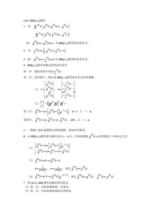
§10.2 GM(1,1)模型 1．设：()()()()()()()⎪⎭⎫ ⎝⎛=n x x xX0000,,2,1()()()()()()()⎪⎭⎫ ⎝⎛=n x x xX1111,,2,1称：()()()()b k a k x x =+10 为GM(1,1)模型的原始形式。

2．令：()()()()()()⎪⎭⎫ ⎝⎛-+=121111k k k xxz3．称：()()()()b k a k z x =+10为GM(1,1)模型的基本形式。

4．GM(1,1)模型求解过程的基本程序 第一步，根据原始序列求()()k z 1。

第二步，利用最小二乘法求GM(1,1)模型基本形式的参数解。

（1）()()()()()()⎥⎥⎥⎥⎥⎥⎦⎤⎢⎢⎢⎢⎢⎢⎣⎡=n Y xx x 00032，()()()()()()⎥⎥⎥⎥⎥⎥⎦⎤⎢⎢⎢⎢⎢⎢⎣⎡---=11312111n B zz z（2）⎥⎦⎤⎢⎣⎡b a ＝()YBB B TT1-第三步，()()()()ab a b k exx at+⎥⎦⎤⎢⎣⎡-=+-1101ˆ，k ＝1，2，…，n 。

第四步，()()()()()()k k k xxx ˆˆˆ11011-+=+， k=1，2，…，n 。

5．一般输入输出建模称为黑箱建模，例如回归模型。

6．由GM(1,1)模型基本解法求出a ，b 后，对原始数据()()10+k x 的预测有三种表达方法。

（1）()()()()()()()()()()⎪⎪⎩⎪⎪⎨⎧-+=++⎥⎦⎤⎢⎣⎡-=+-k k k a ba b k xx x e x x atˆˆˆˆ11011111 （2）()()()()1ˆˆ10--=k k xx αβab5.01+=β，aa5.01+=α，规定()()()()1100ˆxx =（3）()()()()()exx k a k 2001ˆˆ--⎪⎭⎫ ⎝⎛-=αβ，规定()()()()1100ˆxx =，()()()()2200ˆxx =7．例10.2.1 GM 模型求解的规范要求 （1）第一步，对原始数据做一次累加。

目录1研究概述 (1)1.1研究背景 (1)1.2基本思路 (2)1.3创新点 (2)1.4研究贡献 (2)2制度背景 (3)3提出假说 (3)3.1盈余管理假设 (3)3.2调查期间 (4)3.3局限 (4)4样本选择 (4)4.1样本选择 (4)4.2变量选择 (5)5琼斯模型 (5)5.1基本原理 (5)5.2具体操作 (6)6研究结论 (7)7模型评价 (7)1 研究概述1.1 研究背景图1-1 研究背景1） 进口援助进口援助的规则中公开使用的会计数字给经理人员提供了盈余管理的动机，目的是提高获得进口援助的可能性和或提高援助的数量。

进口援助调查提供了一个具体的盈余管理的动机,这是在其他的盈余管理研究中没有的。

ITC 没有根据使用的会计程序或者根据公司制定的关于应计利润的决策调整财务数据。

2）Heal 模型Heal(1985)假设预期非操纵性应计利润等于零，总应计的任何非零值归于管理层操纵。

3）DeAngelo 模型DeAngelo(1986)假设非操纵性应计利润服从随机游走过程。

也就是，对于一个稳定状态的企业，t 时的非操纵性应计利润被假设等于t 一1时的非操纵性应计，因而t 时与t 一1时总应计之间的差异被归于会计操纵。

1/-=it it it TA TA EDA 11/)(---=ititit it A TA TA EDA1.2图1-2 基本思路1.3创新点1）进口援助调查提供了一个具体的盈余管理的动机，这是在其他的盈余管理研究中没有的。

2）对总体应计利润中的操纵性的部分的估计被用作盈余管理的测度变量，而不是使用单一应计利润中的操纵性应计利润部分。

3）公司特征（firm-specific）期望模型被发展成为估计正常（非操纵性的）应计利润。

4）本文发展使用的方法扩展了其他盈余管理研究中的方法；尤其是，时间序列模型被发展用来估计总体非操纵性应计利润，盈余管理假设使用了截面检验。

1.4研究贡献琼斯（1991）发现，被调查的企业为了调减收益而调整应计项目。

对可操控和不可操控的会计应计量信息反映的检验虽然会计应计量和现金流量所带来的会计盈余的持久性具有显著的差异，但是中国的股票价格并没有能够有效地区分这种差异。

本文将讨论导致这种持久性差异的原因以及这种差异是否反映了会计盈余管理的行为。

为此，将利用横截面数据，采用修正的Jones模型将会计应计量分解为可操控的会计应计量和不可操控的会计应计量，然后根据Mishkin理性预期检验方法，讨论中国股票市场是否充分反应了可操控和不可操控会计应计量的差异。

此外本文还将讨论不同的估计方法和预期收益率均衡模型是否会对估算可操控和不可操控会计应计量产生显著的影响。

假设的提出由于权责发生制和配比原则的要求，致使会计盈余和现金流量（在本文而言就是营业利润和经营活动产生的净现金流量）之间产生了差异，也就是存在会计应计量。

但影响会计应计量的因素很多，如固定资产的折旧、无形资产的摊销、销售形成的应收账款、待摊费用、采购形成的应付账款、预提费用等等。

有些账目如固定资产的折旧和无形资产的摊销以及符合公司信用政策的应收账款等是公司持续经营的条件，这些会计应计量的持续性比较强，与公司的营业利润的关系也比较密切，不大容易被公司管理层操纵，而有些项目如资产和债务重组发生的费用和收益、改变会计政策、特殊补贴和带处理的损益等则比较容易受到公司管理层的操纵，持续性也比较弱。

会计应计项目所具有的不同性质也正是应用各种识别可操控和不可操控的会计应计量的方法和模型的前提条件。

据此所要检验的第一个假设（H1）是：根据识别和区分会计应计量的模型所获得的可操控和不可操控的会计应计量所产生的会计盈余的持久性具有显著的不同，不可操控的会计应计量产生的会计盈余比可操控的会计应计量产生的会计盈余的持久性要强。

若该假设成立，会计应计量与现金流量之间的持久性的差异可能主要归之于可操控的会计应计量。

无论可操控的会计应计量和不可操控的会计应计量的持久性是否具有显著的差异，上市公司的股票价格是否理性或者说有效地反映了这两者对会计盈余的持久性都是一个需要再讨论的问题。