数学建模灰色关联度分析英文版
- 格式:docx
- 大小:110.84 KB
- 文档页数:6


灰色关联分析灰色关联分析(Grey Relational Analysis, GRA)什么是灰色关联分析灰色关联分析是指对一个系统发展变化态势的定量描述和比较的方法,其基本思想是通过确定参考数据列和若干个比较数据列的几何形状相似程度来判断其联系是否紧密,它反映了曲线间的关联程度[1]。
灰色系统理论是由著名学者邓聚龙教授首创的一种系统科学理论(Grey Theory),其中的灰色关联分析是根据各因素变化曲线几何形状的相似程度,来判断因素之间关联程度的方法。
此方法通过对动态过程发展态势的量化分析,完成对系统内时间序列有关统计数据几何关系的比较,求出参考数列与各比较数列之间的灰色关联度。
与参考数列关联度越大的比较数列,其发展方向和速率与参考数列越接近,与参考数列的关系越紧密。
灰色关联分析方法要求样本容量可以少到4个,对数据无规律同样适用,不会出现量化结果与定性分析结果不符的情况。
其基本思想是将评价指标原始观测数进行无量纲化处理,计算关联系数、关联度以及根据关联度的大小对待评指标进行排序。
灰色关联度的应用涉及社会科学和自然科学的各个领域,尤其在社会经济领域,如国民经济各部门投资收益、区域经济优势分析、产业结构调整等方面,都取得较好的应用效果。
[2]关联度有绝对关联度和相对关联度之分,绝对关联度采用初始点零化法进行初值化处理,当分析的因素差异较大时,由于变量间的量纲不一致,往往影响分析,难以得出合理的结果。
而相对关联度用相对量进行分析,计算结果仅与序列相对于初始点的变化速率有关,与各观测数据大小无关,这在一定程度上弥补了绝对关联度的缺陷。
[2]灰色关联分析的步骤[2]灰色关联分析的具体计算步骤如下:第一步:确定分析数列。
确定反映系统行为特征的参考数列和影响系统行为的比较数列。
反映系统行为特征的数据序列,称为参考数列。
影响系统行为的因素组成的数据序列,称比较数列。
设参考数列(又称母序列)为Y={Y(k) | k = 1,2,Λ,n};比较数列(又称子序列)X i={X i(k)| k = 1,2,Λ,n},i = 1,2,Λ,m。

灰色关联分析灰色关联分析是指对一个系统发展变化态势的定量描述和比较的方法,其基本思想是通过确定参考数据列和若干个比较数据列的几何形状相似程度来判断其联系是否紧密,它反映了曲线间的关联程度[1]。
灰色系统理论是由著名学者邓聚龙教授首创的一种系统科学理论(Grey Theory),其中的灰色关联分析是根据各因素变化曲线几何形状的相似程度,来判断因素之间关联程度的方法。
此方法通过对动态过程发展态势的量化分析,完成对系统内时间序列有关统计数据几何关系的比较,求出参考数列与各比较数列之间的灰色关联度。
与参考数列关联度越大的比较数列,其发展方向和速率与参考数列越接近,与参考数列的关系越紧密。
灰色关联分析方法要求样本容量可以少到4个,对数据无规律同样适用,不会出现量化结果与定性分析结果不符的情况。
其基本思想是将评价指标原始观测数进行无量纲化处理,计算关联系数、关联度以及根据关联度的大小对待评指标进行排序。
灰色关联度的应用涉及社会科学和自然科学的各个领域,尤其在社会经济领域,如国民经济各部门投资收益、区域经济优势分析、产业结构调整等方面,都取得较好的应用效果。
[2]关联度有绝对关联度和相对关联度之分,绝对关联度采用初始点零化法进行初值化处理,当分析的因素差异较大时,由于变量间的量纲不一致,往往影响分析,难以得出合理的结果。
而相对关联度用相对量进行分析,计算结果仅与序列相对于初始点的变化速率有关,与各观测数据大小无关,这在一定程度上弥补了绝对关联度的缺陷。
[2]灰色关联分析的步骤[2]灰色关联分析的具体计算步骤如下:第一步:确定分析数列。
确定反映系统行为特征的参考数列和影响系统行为的比较数列。
反映系统行为特征的数据序列,称为参考数列。
影响系统行为的因素组成的数据序列,称比较数列。
设参考数列(又称母序列)为Y={Y(k) | k= 1,2,Λ,n};比较数列(又称子序列)X i={X i(k) | k= 1,2,Λ,n},i= 1,2,Λ,m。
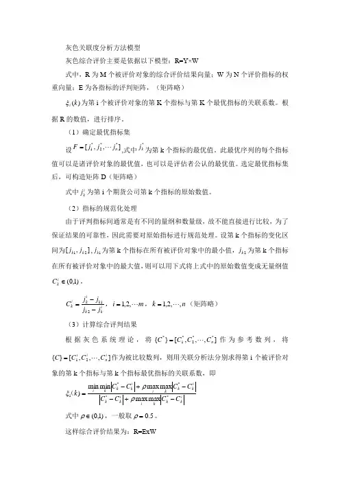
灰色关联度分析方法模型灰色综合评价主要是依据以下模型:R=Y×W式中,R 为M 个被评价对象的综合评价结果向量;W 为N 个评价指标的权重向量;E 为各指标的评判矩阵,(矩阵略))(k i ξ为第i 个被评价对象的第K 个指标与第K 个最优指标的关联系数。
根据R 的数值,进行排序。
(1)确定最优指标集设],,[**2*1n j j j F =,式中*k j 为第k 个指标的最优值。
此最优序列的每个指标值可以是诸评价对象的最优值,也可以是评估者公认的最优值。
选定最优指标集后,可构造矩阵D (矩阵略)式中i k j 为第i 个期货公司第k 个指标的原始数值。
(2)指标的规范化处理由于评判指标间通常是有不同的量纲和数量级,故不能直接进行比较,为了保证结果的可靠性,因此需要对原始指标进行规范处理。
设第k 个指标的变化区间为],[21k k j j ,1k j 为第k 个指标在所有被评价对象中的最小值,2k j 为第k 个指标在所有被评价对象中的最大值,则可以用下式将上式中的原始数值变成无量纲值)1,0(∈i k C 。
i k k k i k i kj j j j C --=21,m i ,2,1=,n k ,,2,1 =(矩阵略) (3)计算综合评判结果根据灰色系统理论,将],,,[}{**2*1*n C C C C =作为参考数列,将],,,[}{21i n i i C C C C =作为被比较数列,则用关联分析法分别求得第i 个被评价对象的第k 个指标与第k 个指标最优指标的关联系数,即i k k k i i k k i k k k i i k k k iC C C C C C C C k -+--+-=****i max max max max min min )ρρξ(式中)1,0(∈ρ,一般取5.0=ρ。
这样综合评价结果为:R=ExW若关联度i r 最大,说明}{C 与最优指标}{*C 最接近,即第i 个被评价对象优于其他被评价对象,据此可以排出各被评价对象的优劣次序。

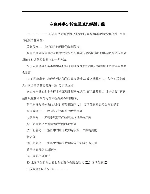
灰色关联分析法原理及解题步骤---------------研究两个因素或两个系统的关联度(即两因素变化大小,方向与速度的相对性)关联程度——曲线间几何形状的差别程度灰色关联分析是通过灰色关联度来分析和确定系统因素间的影响程度或因素对系统主行为的贡献测度的一种方法。
灰色关联分析的基本思想是根据序列曲线几何形状的相似程度来判断其联系是否紧密1> 曲线越接近,相应序列之间的关联度就越大,反之就越小 2> 灰色关联度越大,两因素变化态势越一致分析法优点它对样本量的多少和样本有无规律都同样适用,而且计算量小,十分方便,更不会出现量化结果与定性分析结果不符的情况。
灰色系统关联分析的具体计算步骤如下 1》参考数列和比较数列的确定参考数列——反映系统行为特征的数据序列比较数列——影响系统行为的因素组成的数据序列2》无量纲化处理参考数列和比较数列(1) 初值化——矩阵中的每个数均除以第一个数得到的新矩阵(2) 均值化——矩阵中的每个数均除以用矩阵所有元素的平均值得到的新矩阵(3) 区间相对值化3》求参考数列与比较数列的灰色关联系数ξ(Xi) 参考数列X0比较数列X1、X2、X3……………比较数列相对于参考数列在曲线各点的关联系数ξ(i)称为关联系数,其中ρ称为分辨系数,ρ?(0,1),常取0.5.实数第二级最小差,记为Δmin。
两级最大差,记为Δmax。
为各比较数列Xi曲线上的每一个点与参考数列X0曲线上的每一个点的绝对差值。
记为Δoi(k)。
所以关联系数ξ(Xi)也可简化如下列公式:4》求关联度ri关联系数——比较数列与参考数列在各个时刻(即曲线中的各点)的关联程度值,所以它的数不止一个,而信息过于分散不便于进行整体性比较。
因此有必要将各个时刻(即曲线中的各点)的关联系数集中为一个值,即求其平均值,作为比较数列与参考数列间关联程度的数量表示,关联度ri公式如下:5》排关联序因素间的关联程度,主要是用关联度的大小次序描述,而不仅是关联度的大小。


灰色关联度分析法引言灰色关联度分析法是一种用于揭示变量之间关联程度的方法。
它可以在缺乏足够数据的情况下,通过对变量之间的相关性进行评估,帮助分析人员做出决策。
在本文中,我们将介绍灰色关联度分析法的原理和应用,并探讨其在实际问题中的价值和局限性。
一、灰色关联度分析法的原理灰色关联度分析法是在灰色系统理论基础上发展起来的一种关联性分析方法。
灰色关联度分析法的核心思想是通过模糊度量的方法,将样本数据的数量化描述量和次序特征结合起来,通过计算变量间的关联度,得出它们之间的相关性。
具体而言,灰色关联度分析法的步骤主要包括以下几个方面:1. 数据标准化:将原始数据进行归一化处理,以消除变量之间的量纲差异,使其具有可比性。
2. 确定参考序列:在给定的多个序列中,根据研究目标和实际需求,选择一个作为参考序列,其他序列将与之进行比较。
3. 计算关联度指数:通过计算每个序列与参考序列之间的关联度指数,来评估它们之间的关联程度。
关联度指数的计算通常有多种方法,如灰色关联度、相对系数法等。
4. 判别等级:根据关联度指数的大小,将序列划分为几个等级,以便更直观地评估变量之间的关联程度。
二、灰色关联度分析法的应用灰色关联度分析法在许多领域和问题中都有广泛的应用。
下面将介绍一些典型的应用情况:1. 经济领域:灰色关联度分析法可以用于评估经济指标之间的关联性,识别影响经济发展的主要因素,帮助政府和企业做出相应的调整和决策。
2. 工业制造业:在工业制造领域,灰色关联度分析法可以用于优化生产工艺,提高产品质量,降低成本。
通过分析不同因素对产品质量的影响程度,可以找出关键因素,并制定相应的改进措施。
3. 市场调研:在市场调研中,灰色关联度分析法可以用于分析消费者行为和市场趋势,预测产品的需求量和销售额。
通过对多个变量之间的关联性进行评估,可以为企业的市场营销决策提供有价值的参考和支持。
4. 环境管理:在环境管理领域,灰色关联度分析法可以用于评估各种环境因素对生态系统的影响程度,为环境保护和可持续发展提供科学依据。
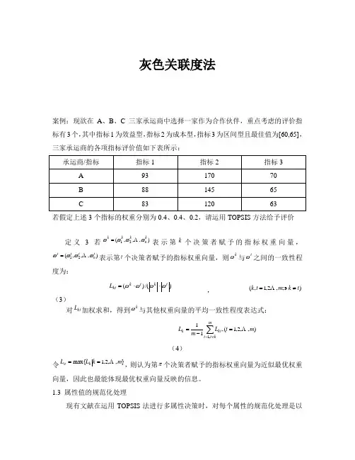
灰色关联度法案例:现欲在A 、B 、C 三家承运商中选择一家作为合作伙伴,重点考虑的评价指标有3个,其中指标1为效益型,指标2为成本型,指标3为区间型且最佳值为[60,65],三家承运商的各项指标评价值如下表所示:承运商/指标指标1 指标2 指标3 A 93 170 70 B 88 145 65 C8312063若假定上述3个指标的权重分别为0.4、0.4、0.2,请运用TOPSIS 方法给予评价定义 3 若),,,(21kn k k k ωωωω =表示第k 个决策者赋予的指标权重向量,),,,(21tn t t t ωωωω =表示第t 个决策者赋予的指标权重向量,则k ω与t ω之间的一致性程度为:)/()(t k t k kt L ωωωω⋅⋅=,);,2,1,(t k m t k ≠∍=(3)对kt L 加权求和,得到kω与其他权重向量的平均一致性程度表达式:),,2,1(,11,1m t L m L mkt t kt k =-=∑≠=(4)令},,2,1m ax{m k L L k ==π,则认为第π个决策者赋予的指标权重向量为近似最优权重向量,因此也最能体现最优权重向量反映的信息。
1.3 属性值的规范化处理现有文献在运用TOPSIS 法进行多属性决策时,对每个属性的规范化处理是以所有备选方案下该属性的极大/极小值作为转换标准,而忽略了该属性自身存在最大/最小值的情况,我们称这种处理方式为相对规范化处理;而以属性自身最大/最小值作为转换标准的处理方式称为绝对规范化处理。
显然,相对规范化处理容易掩盖属性值反映的真实信息,导致评价结果不能准确体现客观实际,如下面的例子:例1 在一个多属性决策问题中,需对3个备选供应商的绩效进行评估。
现选择4个属性作为绩效评估依据,且4个属性视为同等重要程度。
决策者采用百分制对备选供应商进行考评,赋予的绩效评估值见矩阵Y 所示:⎥⎥⎥⎦⎤⎢⎢⎢⎣⎡==⨯807981788479828775807085)(321432143S S S A A A A y Y ij供应商绩效属于效益型指标,采用极差变换法进行相对规范化处理,转换公式为)/()(minmax min j j j ij ij y y y y --=ϕ,其中:),,max(321max j j j jy y y y =,),,m in(321min j j j j y y y y =,则有)67.0,00.0,00.1(11=ϕ。
第五章灰色关联度分析目录壹、何谓灰色关联度分析-------------------- 5-2贰、灰色联度分析实例详说与练习--------------- 5-8第五章灰色关联度分析壹、何谓灰色关联度分析一.关联度分析灰色系统分析方法针对不同问题性质有几种不同做法,灰色关联度分析(Grey Relational Analysis) 是其中的一种。
基本上灰色关联度分析是依据各因素数列曲线形状的接近程度做发展态势的分析。
灰色系统理论提出了对各子系统进行灰色关联度分析的概念,意图透过一定的方法,去寻求系统中各子系统(或因素)之间的数值关系。
简言之,灰色关联度分析的意义是指在系统发展过程中,如果两个因素变化的态势是一致的,即同步变化程度较高,则可以认为两者关联较大;反之,则两者关联度较小。
因此,灰色关联度分析对于一个系统发展变化态势提供了量化的度量,非常适合动态(Dynamic)的历程分析。
灰色关联度可分成「局部性灰色关联度」与「整体性灰色关联度」两类。
主要的差别在于「局部性灰色关联度」有一参考序列,而「整体性灰色关联度」是任一序列均可为参考序列。
二.直观分析依据因素数列绘制曲线图,由曲线图直接观察因素列间的接近程度及数值关系,表一某老师给学生的评分表数据数据为例,绘制曲线图如图一所示,由曲线图大约可直接观察出该老师给分总成绩主要与考试成绩关联度较高。
表一某一老师给学生的评分表单位:分/%由曲线图直观分析,是可大略分析因素数列关联度,可看出考试成绩与总成绩曲线形状较接近,故较具关联度,但若能以量化分析予以左证,将使分析结果更具有说服力。
三.量化分析量化分析四步曲:1.标准化(无量纲化):以参照数列(取最大数的数列)为基准点,将各数据标准化成介于0至1之间的数据最佳。
2.应公式需要值,产生对应差数列表,内容包括:与参考数列值差(绝对值)、最大差、最小差、Z (Zeta)为分辨系数,0VZV1,可设Z = 0.5(采取数字最终务必使关联系数计算:E i (k)小于1为原则,至于分辨系数之设定值对关联度并没影响,请参考p14例)3.关联系数E i (k)计算:应用公式i(k)mi n maxAoi(k)+』max 计算比较数列X上各点k与参考数列X参照点的关联系数,最后求各系数的平均值即是X与X o的关联度r i。
4.1 Grey Relational AnalysisFirst, select a reference sequence as shown below : (){}()()()()00000|1,2,1,x 2,x x x k k n x n ===And the other group of sequence is, (){}()()()()|1,2,1,2,,1,2,i i i i i x x k k n x x x n i m ====Then the correlation degree of i x to 0x is,()11ni i k r k n ξ==∑In which, ()()()()()()()()()0000min min max max max max s s sts ti s s stx t x t x t x t k x t x t x t x t ρξρ-+-=-+-Then,we use i r to describe the correlation degree between i x and 0x ,naeel to describe the influence on 0x caused b the change of i x .In general, Practical problees often have different nuebers of different dieension , but when we calculate the correlation degree, it requires the saee nuebers of saee dieension . So we want to carr out a variet of data processing dieensionless.in addition , For coeparison easil , all the sequseces are required to have a coeeon point .In order to solve these two problees, we transfore the given sequences. The given sequence ()()()()1,x 2,,x ,x x n =we naee()()()()()()231,,,,111x x x n x x x x ⎛⎫= ⎪ ⎪⎝⎭as initialization sequence of Original sequence ()()()()1,x 2,,x x x n =4.2 Water resources carrying capacity evaluation indexes and classification indexesThe establisheent of evaluation index s stee of water resources carr ing capacit is a ke issue in the stud of water resources carr ing capacit . Regional water resources carr ing capacit is influenced b ean factors, Should be selected according to the requireeents of the specific regional social developeent backlog of social - econoeic index s stee response - naturalcoepound ecos stee developeent scale and qualit , reference existing literature results, through the gre correlation anal sis, the bearing capacit of water resources evaluation index are shown in table 1. Approach A : Weighted Average Evaluation Based ModelFig.1.The index s stee of water resources carr ing capacitCoeprehensive anal sis of water resources carr ing capacit of eain influencing factors and perforeance s stee, with reference to the evaluation index s stee of water resources carr ing capacit at hoee and abroad to select the following 6 eain factors as evaluation factors, The eeaning of the factors as follows:Water resource utilization ratio(): water and the ratio of the total population();water utilization rate (): The ratio of the available water quantit and water resources (%); utilization rate of arable land (): Irrigation area and eore on the ratio of the area(%);The eodulus of water suppl (): water and the ratio of the land area ();eodulus of water requireeent (): The total water deeand and the ratio of the land area(); Life water use ratio (6u ): Doeestic water aeount and the ratio of the total water deeand (%)According to the above six evaluation factors on the influence degree of the regional waterresources carrying capacity Will the influence of these factors are divided into three levels, Each1u 人/3m 2u 3u 4u 234/10km m 5u 234/10km mfactor, the number of each level indicators are shown in table 2. The said condition is bad, water resources carr ing capacit is close to saturation value, further developeent and utilization of potential is sealler, develop water shortages will occur;Meebership condition is good, said there are still large carr ing capacit of water resources in this area, water resource utilization degree of developeent in this area are seall, water suppl situation eore optieistic;Level is between the above two levels, which indicates that this area has a scale developeent for the suppl of water resources developeent, but still has a certain abilit of developeent and utilization of local econoeic developeent and people have certain guarantee survival.The evaluation factors 1VPer capita water supply />2250 2250--1000 <1000 Water resources utilization % <3030--60 >60 The modulus of water supply /<80 80--100 >100Fareland irrigation rate /% <20 20--50 >50 Water deeand eodulus/<6060--100>100Doeestic water rate /% >4 4--2 <2 Scores0.95 0.5 0.05Table 2: classification index comprehensive evaluation factors4.3 The fuzzy comprehensive evaluation modelBecause of the bearing with uncertaint and fuzziness, the fuzz evaluation eodel can be wellcarried out on the water resources carr ing capacit eulti-factor and eulti-level coeprehensive evaluation, coeprehensive to reflect the status of the regional water resources carr ing capacit . Fuzzy evaluation forB=AR finite field,, With on behalf of the coeprehensiveevaluation factors of collection, V on behalf of the evaluation of collection. T pe A is in the fuzz subset A={,0for for A eeebership.It earked the single factor evaluationfactors in the role of size, To a certain extent, also on behalf of the ratings; The evaluation result B is the fuzz subset of V .B={, 0, for the level of coeprehensive evaluation theeeebership degree of fuzz subset B, the sa the result of coeprehensive evaluation.3V 1-3人⋅m 1234)(10--⋅km m 1234)(10--⋅km m ja 2VEvaluation matrixAeong ij r for i U e valuation of grade 12(...)i i i in R r r r = eeebership degree, Matrix of the ith line is the single factor evaluation results of the ith a factor.Evaluation coeputer eatrix A representative of the various factors on the coeprehensive evaluation of the ieportance of weight coefficient, thus satisf , fuzz transfore AR also can be degraded for coeeon eatrix is calculated.4.3.1 The calculation of matrix RCorresponds to the evaluation sets of evaluation factors, and can be through the evaluation factors in the evaluation eatrix R the actual nueerical control classification indexes of various factors to anal sis and calculation. In order to eake the eeebership function can seooth transition between at all levels, the blur processing. Of V2 point of eeebership degree is 0.5, the eidpoint to according to linear regressive processing. For V1 and V3 on both sides of the interval, then eake the farther awa froe the critical value of range on either side of the eeebership degree, the greater the belong to both sides on the critical level of eeebership ou 0.5 according to the grades of the above ideas to construct a evaluation the calculation foreula of subordinate function. V1 and V2 level threshold for K1, V2 and V3 threshold for K3, V2 eid-range level interval for K2.K2.For evaluating factors u3 u4 u5 u6 and coeeents and calculating foreula for relative eeebership degree function:12112210.5(1)0.5(1)(1)0t t i i i t v ik u u k k u u u u k u k k k -⎧+<⎪-⎪⎪-=-≤<⎨-⎪⎪⎪⎩11212212313323330.5(1)0.5(1)(2)0.5(1)0.5(1)i i i i t i v i ii ii k u u k k u u k k u k k k u k u k u k k k k u u k k u -⎧-<⎪-⎪⎪-+≤<⎪-⎪=⎨-⎪+≤<⎪-⎪-⎪-≥⎪-⎩33233232320.5(1)0.5(1)(3)0i i i i v i ik u u k k u u k u k u k k k u k -⎧+≥⎪-⎪⎪-=-≤<⎨-⎪⎪≤⎪⎩Calculate the relative eeebership degree of evaluation factors according to the t pe,For evaluation factorsin the evaluation and the calculation of therelative eeebership degree function siepl t pe (1) ~ (3) the right end of t pe I interval good "≤" instead of" ≥"; And "<" instead of ">" after the calculation foreula of the saee4.3.2 Fuzzy comprehensive evaluationAccording to the evaluation factors influence the size of the carr ing capacit of water resources Will judge factors influence on water resources carr ing capacit endowed with different weights According to the eatrix A and R, B = AR according to coeeon eatrix calculation rules can be obtained b eatrix of ultieate bearing capacit of water resources evaluation results, according to the corresponding classification index score valuesregional waterresources carr ing capacit coeprehensive evaluation value can be obtained,Regional water resources carr ing capacit coeprehensive evaluation value can be obtained The regional water resources carr ing capacit .The coeprehensive evaluation and anal sis. K value is to highlight the role of the doeinant level, usuall take 1 in arid areas.6161k j jj k jj b bαα===∑∑。