Tutorial 7_函数

Tutorial 7: Texture Mapping and Constant BuffersSummaryIn the previous tutorial, we introduced lighting to our project. Now we will build on that by adding textures to our cube. Also, we will introduce the concept of constant buffers, and explain how you can use buffers to speed up processing by minimizing bandwidth usage.在之前的tutorial，我们介绍灯光按照我们的规划。

现在我们将建立给我们的方盒子添加材质贴图。

我们也将介绍连续buffer的概念，解释怎样用buffer去提升过程的速度通过最小化带宽的用法。

The purpose of this tutorial is to modify the center cube to have a texture mapped onto it.这个tutorial的目的是去修改中间的方盒子在它上面添加一个材质贴图。

This tutorial concludes the introduction of the basic concepts in Direct3D 10. The tutorials that follow will build upon these concepts by introducing DXUT, mesh loading, as well as an example of each shader.这个tutorial包括介绍基本的概念在Direct3D，下面通过介绍DXUT建立在这些概念上面。

Source(SDK root)\Samples\C++\Direct3D10\Tutorials\Tutorial07Texture mapping材质贴图Texture mapping refers to the projection of a 2D image onto 3D geometry. We can think of it as wrapping a present, by placing decorative paper over an otherwise bland box. To do this, we have to specify how the points on the surface of the geometry correspond with the 2D image.材质贴图是指在3D几何形体上面投影一个2D图像。

Tutorial:Introduction to Size FunctionsPurposeThe purpose of this tutorial is to introduce you to the use of size functions to control the size of mesh intervals for edges and mesh elements for faces and volumes.Based on their application,there are four types of size functions:fixed,curvature,proximity and meshed.This tutorial shows you how to use these size function types to refine a mesh in regions surrounding a specified entity and how to combine boundary layers and size functions for better mesh quality.PrerequisitesThis tutorial assumes that you are familiar with the GAMBIT interface and have a basic understanding of geometry creation and size functions.If you have not used size functions before,you can refer to Section5.2:Size Functions,in the GAMBIT Modeling Guide(http://www.fl/gambit2/doc/doc f.htm).Problem DescriptionYou will create a rectangular face,an elliptical cylindrical volume and a brick geometry and mesh them using the Fixed,Curvature,and Proximity size functions,respectively.Using a journalfile,you will then create and partially premesh2-D and3-D geometry.You will then use the meshed size function to grow the full mesh from the premeshed sections of the geometry.To create a size function,you need to define the Source and Attachment entities and param-eters such as,Growth rate,Size limit,Start size,Angle,and Cells/gap.The Growth rate and Size limit parameters are common to the four size functions.The additional parameter specific to three size functions,which is the initialization parameter used to create mesh on the source entities,is listed below:Type of Size Function Parameter Specific to the FunctionFixed Start sizeCurvature AngleProximity Cells/gapThe meshed size function does not require an initialization parameter,since we are starting from an existing mesh at the source entities.Introduction to Size FunctionsYou can specify more than one size function on any face or volume.Size functions can be used with hexahedral,tetrahedral or hybrid volume meshes and quadilateral or triangular face meshes.Since,you can control the number of elements in mapped or submapped meshes using edge grading,size functions are used in more complex geometries where tetrahedral or Cooper meshing schemes are required.Fixed Size FunctionThe Fixed size function is used to control the maximum mesh-element edge lengths in a model.Step1:Geometry1.Start GAMBIT with the identifier pipe.2.Create a rectangle with the following dimensions:Width Height10103.Create a circle with a value of Radius as1.4.Subtract the circle from the square.(a)In the Subtract Real Faces form,select face.1and face.2for Face and Subtract Facesrespectively.(b)Retain the default values of the other parameters and click Apply.5.Make two copies of the face and translate it.(a)In the Move/Copy Faces form,select face.1for Faces.(b)Select Copy and set the number of copies to2.(c)Under Global,set the value of x:to12.(d)Retain the default values of the other parameters and click Apply.Step2:Mesh the First Face1.Mesh the inner circular loop on thefirst face.(a)In the Mesh Edges form,for Edges,select the edge corresponding to the innercircular loop.(b)Set the Interval size to0.2and click Apply.2.Mesh thefirst face(see Figure1).(a)In the Mesh Faces form,select face.1for Faces and Tri for Elements:.(b)Retain the default values for the other parameters and click Apply.Introduction to Size FunctionsFigure1:Mesh on face.1Step3:Mesh the Second Face Using the Fixed Size Function1.Define afixed type function(fix1)on the second face(face.2).(a)On the Entities:Source:option button,select Edges and select the edge corre-sponding to the inner circular loop.(b)On the Entities:Attachment:option button,select the second face(face.2).(c)Set the values for the remaining parameters as follows:Start size Growth rate Size limit Label0.2 1.50.5fix12.Initialize the size function.(a)In the View Size Function form,selectfix1for S.Function and click Initialize.Note:The Iso-value:ranges from0.2to0.5.You can move the slider bar to examine the extent of the size function.The size function will not encompass the entireface.In the region excluded by the isovalues from0.2to0.5,the elements willhave a constant size of0.5.3.Mesh the second face.(a)Select face.2for Faces and Tri for Elements:.(b)Click Apply.The mesh obtained is muchfiner than the mesh on thefirst face because the valueof Size limit was specified as0.5.Introduction to Size Functions4.Delete the mesh on the second face.You will now adjust the size function parameters to get a coarser mesh on the secondface.5.Modify the size function(fix1)on the second face.(a)Change the value of Size limit to1and retain the default values of the otherparameters.6.Reinitialize the size function.Note:The Iso-value:now ranges from0.2to1.You can move the slider bar to examine the extent of the size function.The size function will not encompass theentire face.In the region excluded by the isovalues from0.2to1,the elementswill have a constant size of1.7.Remesh the second face(see Figure2).With the modified size function,you get a coarser mesh on the second face.Figure2:Mesh on face.2Step4:Mesh the Third Face Using the Fixed Size Function1.Define afixed type function(fix2)on the third face.(a)Set the Source:to the edge corresponding to the inner circular loop.(b)Set the Attachment:to face.3.(c)Set the values for the remaining parameters as follows:Start size Growth rate Size limit Label0.2 1.21fix2Introduction to Size Functions2.Initialize the size function.(a)In the View Size Function form,selectfix2for S.Function and click Initialize.Note:The Iso-value:ranges from0.2to1.You can move the slider bar to examine the extent of the size function.The size function will encompass the entire face.In the region excluded by the isovalues from0.2to1,the elements will have aconstant size of1.3.Mesh the third face with Tri elements.Figure3:Mesh on face.3You can compare the meshes shown in Figures1,2,and3.All the three meshes have the same mesh sizes on the edges,but the meshes created using a size function have a prescribed growth rate that results in fewer elements.Introduction to Size FunctionsCurvature Size FunctionThe Curvature size function controls the angles between the normals for adjacent mesh ele-ments and is useful when the model contains highly curved surfaces.Step1:Geometry1.Delete the previously created faces(face.1,face.2,and face.3).2.Create an elliptical cylinder with the following parameters:Height Radius1Radius2Axis Location1025Centered Z3.Make two copies of the elliptical cylinder and translate them.(a)In the Move/Copy Volumes form,select volume.1for Volumes and set the numberof copies to2.(b)Under Global,set the value of y:to12and x:and z:to0.(c)Retain the default values of the other parameters and click Apply.Step2:Mesh the First Volume1.In the Mesh Volumes form,select volume.1for Volumes and Tet/Hybrid for Elements:.2.Set the Interval size to2and click Apply.Figure4:Mesh on volume.1The mesh poorly represents the model in the regions where the edges are highly curvedand the surfaces are non planar.Introduction to Size Functions Step3:Mesh the Second Volume Using the Curvature Size Function1.Define a curvature type function(curv1).(a)Select Curvature for Type:.(b)On the Entities:Source:option button,select Faces and select the lateral face ofvolume.2.(c)On the Entities:Attachment:option button,select Volumes and select the volumeas volume.2.(d)Set the values for the remaining parameters as follows:Angle Growth rate Size limit Label40 1.22curv12.Mesh the second volume(volume.2)using tetrahedral elements.Figure5:Mesh on volume.2Now,the mesh is a much better approximation of the model where the regions are highly curved.Introduction to Size FunctionsStep4:Mesh the Third Volume Using the Curvature Size Function1.Define a curvature type function(curv2)on the third volume(volume.3).(a)Set the Source:to the lateral face of volume.3and the Attachment:to volume.3.(b)Change the value of Angle to20,and refer to the definition of curv1for values ofthe other parameters.2.Mesh the third volume(volume.3)using tetrahedral elements.Figure6:Mesh on volume.3pare the meshes for the second and third volume(see Figure7).The value of the angle determines the maximum angle between the normal vectors to adjacent mesh elements.Thus,a smaller angle(20degrees)will produce a better approximation toa curved edge than a larger angle(40degrees).Introduction to Size FunctionsFigure7:Magnified View of the Curved Edges of volume.3and volume.2Introduction to Size FunctionsProximity Size FunctionThe Proximity size function controls the number of mesh elements in faces between two geometric entities and is useful when there are small gaps in the model.Step1:Geometry1.Delete the previously created volumes(volume.1,volume.2and volume.3).2.Create a brick with the following dimensions:Width Depth Height Direction555Centered3.Create a thinner brick with the following dimensions:Width Depth Height Direction0.255Centered4.Move the thinner brick.(a)In the Move/Copy Volumes form,select volume.2or Volumes,and under Global,setthe values of x:to2,y:to0,and z:to2.5.5.Subtract the thinner brick from the larger brick.(a)In the Subtract Real Volumes form,select volume.1for Volume and volume.2forSubtract Volumes and click Apply.Figure8:Subtracted Volume(volume.1)There is a thin rectangular face(face.11)and a small gap of0.4width within thevolume bounded by the faces,face.13and face.1.6.Make a copy of the volume and translate it.(a)In the Move/Copy Volumes form,select volume.1for Volumes and set the numberof copies to1.(b)Under Global,set the value of x:to6,and y:and z:to0.(c)Retain the default values of the other parameters and click Apply.Step2:Mesh the First Volume Using Proximity Size Function1.Define a proximity type function(prox1)on thefirst volume(volume.1).(a)Select Proximity for Type:.(b)On the Entities:Source:option button,select Faces and select the thin rectangularface(face.11)of volume.1.(c)On the Entities:Attachment:option button,select Volumes and select the volumeas volume.1.(d)Set the values for the remaining parameters as follows:Cells/gap Growth rate Size limit Label3 1.31prox12.Mesh volume.1using tetrahedral elements.Figure9:Mesh on volume.1Figure10:Magnified View of Mesh on volume.1There are3elements in the thin rectangular face(face.11),however there is only one element in the thin gap bounded by the faces,face.13and face.1.Step3:Mesh the Second Volume Using Proximity Size Function1.Define a proximity function(prox2)on the second volume.(a)Set the Source:to the three faces(face.17,face.16,and face.25)of volume.2.(b)Set the Attachment:to volume.2,and refer to the definition of prox1for values ofthe other parameters.2.Mesh volume.2using tetrahedral elements.Now,there are3elements in the thin rectangular face(face.17)and three elements in the thin gap bounded by the faces,face.16,and face.25(see Figure12).Figure11:Mesh on volume.2Figure12:Magnified View of Mesh on volume.2Meshed Size FunctionThe meshed size function is used to grow mesh from source entities,which have been premeshed.This size function can be used for growing a graded surface mesh from pre-meshed edges or graded volume meshes from premeshed faces.You will need the journal file,meshed-sf-prep.jou for this section.Step1:Geometry and Premeshing using a Journal File1.Start GAMBIT with the identifier meshed-sf.2.In the File menu,select Run Journal....3.In the Run Journal form,select the Edit/Run mode.4.Click Browse...and navigate to the directory containing the journalfile meshed-sf-prep.jou.5.Select thefile meshed-sf-prep.jou and click Accept.6.In the Edit/Run Journal form,right-click the mouse and choose Select All in the drop-down menu.7.Click Step repeatedly to execute the commands in the journalfile one after another. Note:Observe the sequence of events on the screen from geometry creation to meshing ofedges and face.You may need to click the button to view all geometry.Step2:Mesh the First Face Using a Meshed Size Function1.Create a meshed size function with source as the edges and attachment entity asface.1.(a)Select Meshed as Type:.(b)On the Entities:Source:option button,select Edges and select all four premeshededges of thefirst face.(c)On the Entities:Attachment:option button,select thefirst face(face.1).(d)Set the values of the parameters as follows:Growth Rate Size Limit Label1.12meshed12.Mesh the face with quadrilaterals using the quad pave scheme.Figure13:Face Meshed Using Quad Pave SchemeIt can be observed that the mesh grows into the face from the edge meshes(Figure13).The face mesh can be made smoother orfiner by adjusting the growth rate and the size limit.This is useful for meshing complex faces containing edge meshes with different grading and spacing.Step3:Mesh the Volume Using a Meshed Size Function3.Create a meshed size function with source as the meshed face and attachment entityas volume.(a)Select Meshed as Type:.(b)On the Entities:Source:option button,select the Faces and select the premeshedface of the volume.(c)On the Entities:Attachment:option button,select Volume and select the volume(volume.1).(d)Set the values of the parameters as follows:Growth Rate Size Limit Label1.24meshed24.Mesh the volume with a Tet/Hybrid mesh using the Tgrid meshing scheme.Figure14:Cross-Sectional View of Mesh Along Length of the Volume It can be observed that the mesh grows from the premeshed face into the volume(Fig-ure14).The mesh can be changed by changing the growth rate and the size limit.This is useful in ensuring a smooth transition in mesh between different sections of a larger geometry or in growing a volume mesh from premeshed complex surfaces.In addition, the meshed sizing function can be used for creating a volume mesh grown from the end-capping surface of a prismatic boundary layer grown from surface meshes.Combining the Size Function and Boundary LayerSizing functions can also be combined with boundary layers.In the following example,the volume contains an interior void and the boundary layer must be attached to all the interior faces of this void.In this case,the internal continuity must be turned on.Step1:Geometry1.Delete the previously created volumes(volume.1and volume.2).2.Create a brick with the following dimensions:Width Depth Height Direction141414Centered3.Create an elliptical cylinder with the following parameters:Height Radius1Radius2Axis Location513Centered Z4.Subtract the cylinder from the brick.5.Make two copies of the subtracted volume and translate it.(a)Under Global,set the value of x:to16and y:and z:to0.Step2:Mesh the First Volume Using Size Functions1.Define a curvature type function curvbl1on thefirst volume(volume.1).(a)Select Curvature for Type:.(b)On the Entities:Source:option button,select Faces and select the lateral face ofthe cylinder.(c)On the Entities:Attachment:option button,select Volumes and select the volumeas volume.1.(d)Set the values for the remaining parameters as follows:Angle Growth rate Size limit Label30 1.31curvbl12.Mesh the volume using tetrahedral elements.3.Examine the mesh(see Figure15).(a)Set the Display Type:to Plane and select the tetrahedral3D Element.Figure15:Slice of the Mesh in the z directionStep3:Mesh the Second Volume Using Size Functions and Boundary Layer1.Define a curvature type function(curvbl2)on the second volume using the definitionfor curvbl1.2.Create a boundary layer for volume.2using the Uniform algorithm.(a)Set the values of the following parameters:First row Growth factor Rows0.2 1.23(b)Turn on Internal continuity.(c)Define the three faces(face.16,face.17,and face.18)of the cylinder as the At-tachment:.(d)Retain the default values for the other parameters and click Apply.3.Mesh the volume using tetrahedral elements.4.Examine the mesh.(a)Set the Display Type:to Plane and select the wedge3D Element.(b)Slide the slider bar in the Z direction(see Figure16).As you have used the uniform based boundary layer,you will see that the heightof thefirst layer of prism elements is constant.Figure16:Magnified View of the Prism Elements in the Boundary Layer(c)Select the tetrahedral3D Element and examine the growth of the elements out-wards from the interior void(see Figure17).Figure17:Slice of the mesh in the z directionStep4:Mesh the Third Volume Using Size Functions and Boundary Layer1.Define a curvature type function(curvbl3)on the third volume using the definition forcurvbl1.2.Create a boundary layer for volume.3using the Aspect ratio based algorithm.(a)Set the values of the following parameters:First percent Growth factor Rows30 1.23(b)Turn on Internal continuity.(c)Define the three faces(face.25,face.26,and face.27)of the cylinder as the At-tachment:.3.Mesh the volume using tetrahedral elements.4.Examine the mesh.(a)Set the Display Type:to Plane and select the wedge3D Element.(b)Slide the slider bar in the Z direction(see Figure18).Figure18:Magnified View of the Prism Elements in the Boundary LayerAs you have used the aspect ratio based boundary layer,you will see that theheight of thefirst layer of prism elements is not constant.Introduction to Size Functions(c)Select the tetrahedral3D Element and examine the growth of the elements out-wards from the interior void(see Figure19).Figure19:Slice of the Mesh in the z directionc Fluent Inc.June3,200521。

About the T utorialSciPy, a scientific library for Python is an open source, BSD-licensed library for mathematics, science and engineering. The SciPy library depends on NumPy, which provides convenient and fast N-dimensional array manipulation. The main reason for building the SciPy library is that, it should work with NumPy arrays. It provides many user-friendly and efficient numerical practices such as routines for numerical integration and optimization.This is an introductory tutorial, which covers the fundamentals of SciPy and describes how to deal with its various modules.AudienceThis tutorial is prepared for the readers, who want to learn the basic features along with the various functions of SciPy. After completing this tutorial, the readers will find themselves at a moderate level of expertise, from where they can take themselves to higher levels of expertise.PrerequisitesBefore proceeding with the various concepts given in this tutorial, it is being expected that the readers have a basic understanding of Python. In addition to this, it will be very helpful, if the readers have some basic knowledge of other programming languages.SciPy library depends on the NumPy library, hence learning the basics of NumPy makes the understanding easy.Copyright and DisclaimerCopyright 2017 by Tutorials Point (I) Pvt. Ltd.All the content and graphics published in this e-book are the property of Tutorials Point (I) Pvt. Ltd. The user of this e-book is prohibited to reuse, retain, copy, distribute or republish any contents or a part of contents of this e-book in any manner without written consent of the publisher.We strive to update the contents of our website and tutorials as timely and as precisely as possible, however, the contents may contain inaccuracies or errors. Tutorials Point (I) Pvt. Ltd. provides no guarantee regarding the accuracy, timeliness or completeness of our website or its contents including this tutorial. If you discover any errors on our website or in this tutorial, please notify us at **************************T able of ContentsAbout the Tutorial (i)Audience (i)Prerequisites (i)Copyright and Disclaimer (i)Table of Contents (ii)1.SciPy – Introduction (1)2.SciPy – Environment Setup (3)3.SciPy – Basic Functionality (4)NumPy Vector (4)Intrinsic NumPy Array Creation (4)Matrix (6)4.SciPy – Cluster (7)K-Means Implementation in SciPy (7)Compute K-Means with Three Clusters (8)5.SciPy – Constants (10)SciPy Constants Package (10)List of Constants Available (10)6.SciPy – Fftpack (14)Fast Fourier Transform (14)Discrete Cosine Transform (15)7.SciPy – Integrate (17)Single Integrals (18)Multiple Integrals (18)Double Integrals (18)8.SciPy – Interpolate (20)What is Interpolation? (20)1-D Interpolation (21)Splines (22)9.SciPy – Input & Output (25)10.SciPy – Linalg (27)Linear Equations (27)Finding a Determinant (28)Eigenvalues and Eigenvectors (29)Singular Value Decomposition (29)11.SciPy – Ndimage (31)Opening and Writing to Image Files (31)Filters (35)Edge Detection (37)12.SciPy – Optimize (40)Nelder–Mead Simplex Algorithm (40)Least Squares (41)Root finding (42)13.SciPy – Stats (44)Normal Continuous Random Variable (44)Uniform Distribution (45)Descriptive Statistics (46)T-test (47)14.SciPy – CSGraph (49)Graph Representations (49)Obtaining a List of Words (51)15.SciPy – Spatial (54)Delaunay Triangulations (54)Coplanar Points (55)Convex hulls (55)16.SciPy – ODR (57)17.SciPy – Special Package (60)1.SciPySciPy, pronounced as Sigh Pi, is a scientific python open source, distributed under the BSD licensed library to perform Mathematical, Scientific and Engineering Computations.The SciPy library depends on NumPy, which provides convenient and fast N-dimensional array manipulation. The SciPy library is built to work with NumPy arrays and provides many user-friendly and efficient numerical practices such as routines for numerical integration and optimization. Together, they run on all popular operating systems, are quick to install and are free of charge. NumPy and SciPy are easy to use, but powerful enough to depend on by some of the world's leading scientists and engineers.SciPy Sub-packagesSciPy is organized into sub-packages covering different scientific computing domains. These are summarized in the following table:SciPyData StructureThe basic data structure used by SciPy is a multidimensional array provided by the NumPy module. NumPy provides some functions for Linear Algebra, Fourier Transforms and Random Number Generation, but not with the generality of the equivalent functions in SciPy.Standard Python distribution does not come bundled with any SciPy module. A lightweight alternative is to install SciPy using the popular Python package installer,If we install the Anaconda Python package, Pandas will be installed by default. Following are the packages and links to install them in different operating systems.WindowsAnaconda(from https://www.continuum.io) is a free Python distribution for the SciPy stack. It is also available for Linux and Mac.Canopy (https:///products/canopy/) is available free, as well as for commercial distribution with a full SciPy stack for Windows, Linux and Mac.Python (x,y): It is a free Python distribution with SciPy stack and Spyder IDE for Windows OS. (Downloadable from http://python-xy.github.io/)LinuxPackage managers of respective Linux distributions are used to install one or more packages in the SciPy stack.UbuntuWe can use the following path to install Python in Ubuntu.FedoraWe can use the following path to install Python in Fedora.By default, all the NumPy functions have been available through the SciPy namespace. There is no need to import the NumPy functions explicitly, when SciPy is imported. The main object of NumPy is the homogeneous multidimensional array. It is a table of elements (usually numbers), all of the same type, indexed by a tuple of positive integers. In NumPy, dimensions are called as axes. The number of axes is called as rank.Now, let us revise the basic functionality of Vectors and Matrices in NumPy. As SciPy is built on top of NumPy arrays, understanding of NumPy basics is necessary. As most parts of linear algebra deals with matrices only.NumPy V ectorA Vector can be created in multiple ways. Some of them are described below.Converting Python array-like objects to NumPyLet us consider the following example.The output of the above program will be as follows.Intrinsic NumPy Array CreationNumPy has built-in functions for creating arrays from scratch. Some of these functions are explained below.Using zeros()The zeros(shape) function will create an array filled with 0 values with the specified shape. The default dtype is float64. Let us consider the following example.The output of the above program will be as follows.Using ones()The ones(shape) function will create an array filled with 1 values. It is identical to zeros in all the other respects. Let us consider the following example.The output of the above program will be as follows.Using arange()The arange() function will create arrays with regularly incrementing values. Let us consider the following example.The above program will generate the following output.Defining the data type of the valuesLet us consider the following example.The above program will generate the following output.Using linspace()The linspace() function will create arrays with a specified number of elements, which will be spaced equally between the specified beginning and end values. Let us consider the following example.The above program will generate the following output.MatrixA matrix is a specialized 2-D array that retains its 2-D nature through operations. It has certain special operators, such as * (matrix multiplication) and ** (matrix power). Let us consider the following example.The above program will generate the following output.Conjugate Transpose of MatrixThis feature returns the (complex) conjugate transpose of self. Let us consider the following example.The above program will generate the following output.Transpose of MatrixThis feature returns the transpose of self. Let us consider the following example.The above program will generate the following output.When we transpose a matrix, we make a new matrix whose rows are the columns of the original. A conjugate transposition, on the other hand, interchanges the row and the column index for each matrix element. The inverse of a matrix is a matrix that, if multiplied with the original matrix, results in an identity matrix.SciPyEnd of ebook previewIf you liked what you saw…Buy it from our store @ https://7。

Python之Numpy库常⽤函数⼤全（含注释）前⾔：最近学习，才发现原来python⾥的各种库才是⼤头！于是乎找了学习资料对Numpy库常⽤的函数进⾏总结，并带了注释。

在这⾥分享给⼤家，对于库的学习，还是⽤到时候再查，没必要死记硬背。

PS：本博⽂摘抄⾃中国慕课⼤学上的课程《Python数据分析与展⽰》，推荐刚⼊门的同学去学习，这是⾮常好的⼊门视频。

Numpy是科学计算库,是⼀个强⼤的N维数组对象ndarray，是⼴播功能函数。

其整合C/C++.fortran代码的⼯具，更是Scipy、Pandas等的基础.ndim ：维度.shape ：各维度的尺度（2，5）.size ：元素的个数 10.dtype ：元素的类型 dtype(‘int32’).itemsize ：每个元素的⼤⼩，以字节为单位，每个元素占4个字节ndarray数组的创建np.arange(n) ; 元素从0到n-1的ndarray类型np.ones(shape): ⽣成全1np.zeros((shape)， ddtype = np.int32) ：⽣成int32型的全0np.full(shape, val): ⽣成全为valnp.eye(n) : ⽣成单位矩阵np.ones_like(a) : 按数组a的形状⽣成全1的数组np.zeros_like(a): 同理np.full_like (a, val) : 同理np.linspace（1,10,4）：根据起⽌数据等间距地⽣成数组np.linspace（1,10,4, endpoint = False）：endpoint 表⽰10是否作为⽣成的元素np.concatenate():数组的维度变换.reshape(shape) : 不改变当前数组，依shape⽣成.resize(shape) : 改变当前数组，依shape⽣成.swapaxes(ax1, ax2) : 将两个维度调换.flatten() : 对数组进⾏降维，返回折叠后的⼀位数组数组的类型变换数据类型的转换：a.astype(new_type) : eg, a.astype (np.float)数组向列表的转换： a.tolist()数组的索引和切⽚⼀维数组切⽚a = np.array ([9, 8, 7, 6, 5, ])a[1:4:2] –> array([8, 6]) ： a[起始编号：终⽌编号（不含）：步长]多维数组索引a = np.arange(24).reshape((2, 3, 4))a[1, 2, 3] 表⽰ 3个维度上的编号，各个维度的编号⽤逗号分隔多维数组切⽚a [：，：，：：2 ] 缺省时，表⽰从第0个元素开始，到最后⼀个元素数组的运算np.abs(a) np.fabs(a) : 取各元素的绝对值np.sqrt(a) : 计算各元素的平⽅根np.square(a): 计算各元素的平⽅np.log(a) np.log10(a) np.log2(a) : 计算各元素的⾃然对数、10、2为底的对数np.ceil(a) np.floor(a) : 计算各元素的ceiling 值， floor值（ceiling向上取整，floor向下取整）np.rint(a) : 各元素四舍五⼊np.modf(a) : 将数组各元素的⼩数和整数部分以两个独⽴数组形式返回np.exp(a) : 计算各元素的指数值np.sign(a) : 计算各元素的符号值 1（+），0，-1（-）.np.maximum(a, b) np.fmax() : ⽐较（或者计算）元素级的最⼤值np.minimum(a, b) np.fmin() : 取最⼩值np.mod(a, b) : 元素级的模运算np.copysign(a, b) : 将b中各元素的符号赋值给数组a的对应元素数据的CSV⽂件存取CSV (Comma-Separated Value,逗号分隔值) 只能存储⼀维和⼆维数组np.savetxt(frame, array, fmt=’% .18e’, delimiter = None): frame是⽂件、字符串等，可以是.gz .bz2的压缩⽂件； array 表⽰存⼊的数组； fmt 表⽰元素的格式 eg： %d % .2f % .18e ; delimiter：分割字符串，默认是空格eg： np.savetxt(‘a.csv’, a, fmt=%d, delimiter = ‘,’ )np.loadtxt(frame, dtype=np.float, delimiter = None, unpack = False) : frame是⽂件、字符串等，可以是.gz .bz2的压缩⽂件； dtype：数据类型，读取的数据以此类型存储； delimiter: 分割字符串，默认是空格; unpack: 如果为True，读⼊属性将分别写⼊不同变量。

欢迎加入化学化工软件的专业论坛Origin 7.0简明用法李会民lihm@Origin作为一个强大的基于图形化的数据作图软件，尽管其功能非常繁多和强大，但使用起来还是非常简单。

考虑到很多同学没有接触过，我在这里就做一个简单的介绍，其目的主要是为9922和0022的《计算物理》课的数据作图需要服务。

本简明用法仅仅用来供大家对Origin有个大体了解，具体和高级用法还得靠自己捉摸，希望大家能做到举一反三。

我感觉没事了可以随便在那些窗口上双击左键或者单击右键自己玩玩，一般功能可以通过这个学会，但高级功能最好还是看看帮助和资料。

本教程主要参考《Origin 6.0实例教程》（ 晨曦工作室 郝红伟 施光凯 中国电力出版社 2000年8月版）来编写这个简明讲义，在此特表示感谢。

因为自己的经验少，现在就主要按照它这个结构并结合我的一点经验来说说，而且大部分点到为止，如需详细介绍，请自己搜资料或者和我联系，我再补充。

头一次玩讲义，而且很匆忙，会有很多不足之处，还请大家毫不客气地指出，谢谢！目录第一章：Origin基础知识第二章：简单二维图第三章：数据管理第四章：绘制多层图形第五章：非线性拟合第六章：数据分析第七章：绘制三维图形第八章：创建版面页第九章：Origin中Excel的使用第十章：数据的输入输出第十一章：LabTalk 编程部分英文文献：Additions and Improvements to LabTalk 6.1.pdfCategory Reference for LabTalk Commands, Objects, Functions,and Macros.pdf Curve Fitting Functions.pdfOrigin 6.1 Feature List and Tutorial Manual.pdfOrigin 6.1 LabTalk Developer's Guide.pdf仅用于内部交流。

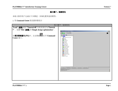
练习题 7: 响应面和优化本练习通过指导用户完成如下任务，细化电子机箱模型：1.定义开孔位置和开孔率（free area ratio）的研究参数2.创建响应面，以确定最佳外形和理解设计的敏感性Tutorial 7 – Response Surfaces and Optimization 本练习将研究改变进口通风位置和开孔率下热性能的敏感性，为了非热设计方面的原因，我们假定需要进一步减小开孔面积。

同时也注意到，模型采用了简化的主板和电源模块，以加速求解，使求解时间控制在培训可接受的范围内，并且，不影响我们研究详细模型的参数和优化。

如果Tutorial 6没有被导入，先要导入（ Load），并另存为 Tutorial 7.输入标题（Title）为“Optimize Venting”Tutorial 7 – Response Surfaces and Optimization 我们首先要做的是将进风口的高度改为 50mm，以减小空气流入的面积首先，调整机箱（Chassis）的High X壁面上孔（Hole）的高度为50 mm.在项目管理（Project Manager）窗口中右击HighX壁面上的孔（Hole），进入Construction 菜单，将尺寸中238 mm 改为50mm，点击OK 退出在出现的网格改变信息窗口中点击‘No’Tutorial 7 – Response Surfaces and Optimization 接着，改变多孔板（Perforated Plate）尺寸，使之和孔的大小一致右击‘High X Perf’，进入Construction 菜单改变尺寸238 mm 为 50 mm.我们还需要改变定义孔的方式，使后面的练习时可以简单地设定参数的变化In the在右图的对话框中，将覆盖（Coverage）设置从间距（Pitch）设定改为开孔率（Free Area Ratio）设置开孔率（Free Area Ratio ）为 0.95.现在，我们在优化模块（Command Center）中可以定义一个变量(the Free Area Ratio) ，不需要定义两个变量(X-Pitch and Y-Pitch).Tutorial 7 – Response Surfaces and Optimization 在绘图板（ Drawing Board）窗口中, 检查一下确保多孔板（Perforated Plate）和开孔（Hole）在相同的位置。

Origin 7.0简明用法Origin 7.0简明用法李会民lihm@Origin作为一个强大的基于图形化的数据作图软件，尽管其功能非常繁多和强大，但使用起来还是非常简单。

考虑到很多同学没有接触过，我在这里就做一个简单的介绍，其目的主要是为9922和0022的《计算物理》课的数据作图需要服务。

本简明用法仅仅用来供大家对Origin有个大体了解，具体和高级用法还得靠自己捉摸，希望大家能做到举一反三。

我感觉没事了可以随便在那些窗口上双击左键或者单击右键自己玩玩，一般功能可以通过这个学会，但高级功能最好还是看看帮助和资料。

本教程主要参考《Origin 6.0实例教程》（ 晨曦工作室 郝红伟 施光凯 中国电力出版社 2000年8月版）来编写这个简明讲义，在此特表示感谢。

因为自己的经验少，现在就主要按照它这个结构并结合我的一点经验来说说，而且大部分点到为止，如需详细介绍，请自己搜资料或者和我联系，我再补充。

头一次玩讲义，而且很匆忙，会有很多不足之处，还请大家毫不客气地指出，谢谢！目录部分英文文献：仅用于内部交流。

第一章 Origin基础知识Origin是美国Microcal公司出的数据分析和绘图软件,现在的最高版本为7.0/特点：使用简单，采用直观的、图形化的、面向对象的窗口菜单和工具栏操作，全面支持鼠标右键、支持拖放式绘图等。

两大类功能：数据分析和绘图。

数据分析包括数据的排序、调整、计算、统计、频谱变换、曲线拟合等各种完善的数学分析功能。

准备好数据后，进行数据分析时,只需选择所要分析的数据,然后再选择响应的菜单命令就可。

Origin的绘图是基于膜板的,Origin本身提供了几十种二维和三维绘图模板而且允许用户自己定制模板。

绘图时,只要选择所需要的模板就行。

用户可以自定义数学函数、图形样式和绘图模板；可以和各种数据库软件、办公软件、图像处理软件等方便的连接；可以用C等高级语言编写数据分析程序，还可以用内置的Lab Talk语言编程等。