Application of the power flow calculation method to islanding micro grids

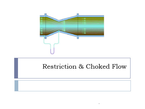
VSSTR-9/05 VALVE SIZING & SELECTION TECHNICAL REFERENCETABLE OF CONTENTSIntroductionValve Flow TerminologyThe Sizing ProcessConditionsOperatingPropertiesFluidRangeabilityC v and Flow Sizing FormulasC V Formulas for Liquid FlowC V Formulas for Vapor FlowC V Formulas for Two Phase FlowFlow Velocity FormulasFlow Velocity for Liquid FlowFlow Velocity for Vapor FlowNomenclatureConversion to Cg and CsSeat LeakageActuator Sizing∆P TablesApplication Guide for Cavitation, Flashing and Compressible Flow ServicesLiquid FlowCavitationDefinitionCavitationCountermeasuresCavitationApplication of Warren Trims in Cavitation ServiceAvoidanceCavitationTolerantCavitationContainmentCavitationPreventionCavitationPhenomenaTheCavitationFluid and Pressure ProfilesChoked Flow and Incipient CavitationDamageCavitationFlashingDefinitionFlashingCountermeasuresFlashingMaterialBodySelectionTrimApplication of Warren Valves in Flashing ServiceBodyMaterial:SelectionTrimPhenomenaTheFlashingLiquid Flow Velocity - Body MaterialCompressible Flow NoiseCompressible Flow Noise DiscussionCompressible Flow Noise CountermeasuresApplication of Warren Trims in Compressible Flow ApplicationsTrims:StandardTrimsMultipleOrificeCompressible Flow Velocity Limits:Two Stage Trims and Backpressure Orifices:The Compressible Flow Noise PhenomenaTABLESTrim Rangeability Table 1Fluid Properties Table 2F L Factors Table 3Flanged Body Inlet and Outlet Diameters Table 4Allowable Seat Leakage Classes Table 5Liquid Flow Velocity Limits Table 6FIGURESCavitationINTRODUCTIONA Control Valve performs a special task, controlling the flow of fluids so a process variable such as fluid pressure, fluid level or temperature can be controlled. In addition to controlling the flow, a control valve may be used to shut off flow. A control valve may be defined as a valve with a powered actuator that responds to an external signal. The signal usually comes from a controller. The controller and valve together form a basic control loop. The control valve is seldom full open or closed but in an intermediate position controlling the flow of fluid through the valve. In this dynamic service condition, the valve must withstand the erosive effects of the flowing fluid while maintaining an accurate position to maintain the process variable.A Control Valve will perform these tasks satisfactorily if it is sized correctly for the flowing and shut-off conditions. The valve sizing process determines the required C V, the required F L, Flow Velocities, Flow Noise and the appropriate Actuator SizeVALVE FLOW TERMINOLOGYC V: The Flow Coefficient, C V, is a dimensionless value that relates to a valve’s flow capacity.Its most basic form is CQPV=∆where Q=Flow rate and ∆P=pressure drop across thevalve. See pages 6, 7 & 9 for the equations for liquid, gas, steam and two phase flow. TheC V value increases if the flow rate increases or if the ∆P decreases. A sizing application will have a Required C V while a valve will have a Rated C V. The valve’s rated C V must equal or exceed the required C V.F L: The F L, Liquid Pressure Recovery Coefficient, is a dimensionless constant used to calculate the pressure drop when the valve’s liquid flow is choked. The F L is the square root of the ratio of valve pressure drop to the pressure drop from the inlet pressure to the pressure of the vena contracta. See page 7 for the F L equation. The F L factor is an indication of the valve’s vena contracta pressure relative to the outlet pressure. If the F L were 1.0, the vena contracta pressure would be the same as the valve’s outlet pressure and there would be no pressure recovery. As the F L value becomes smaller the vena contracta pressure becomes increasingly lower than the valve’s outlet pressure and the valve is more likely to cavitate. A valve’s Rated F L varies with the valve and trim style, it may vary from .99 for a special multiple stage trim to .30 for a ball valve.Rated F L: The Rated F L is the actual F L value for a particular valve and trim style.Required F L: The Required F L is the F L value calculated for a particular service condition. It indicates the required F L needed to avoid choked flow. If the Rated F L is less than the Required F L, the liquid flow will be choked with cavitation.Vena Contracta: The vena contracta is where the jet of flowing fluid is the smallest immediately downstream of the trim's throttle point. At the vena contracta, the fluid's velocity is the highest and the fluid's pressure is the lowest.Vapor Pressure: A fluid's vapor pressure is the pressure where the fluid will change from a liquid to a vapor. The liquid will change to a vapor below the vapor pressure and a vapor willchange to a liquid above the vapor pressure. The vapor pressure increases as the temperature increases.Choked Flow: Liquid flow will become choked when the trim's vena contracta is filled with vapor from cavitation or flashing. Vapor flow also will become choked when the flow velocity at the vena contracta reaches sonic. A choked flow rate is limited; a further decrease of the outlet pressure does not increase flow. Choked flow is also called critical flow.Cavitation: Cavitation is a two stage phenomena with liquid flow. The first stage is the formation of vapor bubbles in the liquid as the fluid passes through the trim and the pressure is reduced below the fluid's vapor pressure. The second stage is the collapse of the vapor bubbles as the fluid passes the vena contracta and the pressure recovers and increases above the vapor pressure. The collapsing bubbles are very destructive when they contact metal parts and the bubble collapse may produce high noise levels.Flashing: Flashing is similar to cavitation except the vapor bubbles do not collapse, as the downstream pressure remains less than the vapor pressure. The flow will remain a mixture of vapor and liquid.Laminar Flow: Most fluid flow is turbulent. However, when the liquid flow velocity is very slow or the fluid is very viscous or both, the flow may become laminar. When the flow becomes laminar, the required C V is larger than for turbulent flow with similar conditions. The ISA sizing formulas adjust the C V when laminar flow exists.THE SIZING PROCESSThe first sizing step is to determine the required C V value for the application. Next determine if there are unusual conditions that may affect valve selection such as cavitation, flashing, high flow velocities or high flow noise. The valve sizing process will determine the proper valve size, valve trim size , valve trim style and actuator size. Warren’s Valve Sizing Program will accurately calculate the C V, flow velocity and flow noise. The program will also show messages when unusual conditions occur such as cavitation, flashing, high velocity or high noise. The results from Warren’s Valve Sizing Program are only one element of the valve selection process. Knowledge and judgment are also required. This overview will give the user some of the sizing basics.The liquid, gas and steam C V calculation methods, in this manual, are in accordance with ISA S75.01 and the gas and steam flow noise calculations are in accordance withISA S75.17. These two ISA Standards are in agreement with IEC-534. These standards have worldwide acceptance as the state of the art in C V and Flow Noise determination. Operating ConditionsThe most important part of Valve Sizing is obtaining the correct flowing conditions. If they are incorrect or incomplete, the sizing process will be faulty. There are two common problems. First is having a very conservative condition that overstates the C V and provide a valve less than ½ open at maximum required flow. The second is stating only the maximum flow condition that has minimum pressure drops and not stating the minimum flow conditions with high-pressure drops that often induce cavitation or have very high rangeability requirements.Fluid PropertiesTable 2 lists many fluid properties needed for valve sizing. These fluid properties are in Warren’s Valve Sizing Program’s database and do not need manual entry.Rangeability: Rangeability is the ratio of maximum to minimum controllable C V. This is also sometimes called C V Ratio or Turndown. The maximum flow for Warren Controls’ valves is at maximum travel. The minimum controllable C V is where the Flow Characteristic (C V vs. Travel) initially deviates or where the valve trim cannot maintain a consistent flow rate. This is partially a function actuator stiffness as well as valve “stiction”. The Trim’s rangeability is not always the useable range as seat erosion may be a governing factor with respect to erosive fluids and high drops in the near-closed position. A valve with a significant pressure drop should not be used to throttle near the seat for extended periods of time.The rangeability values, listed in Table 1, apply to the rated C V, not the required C V. For example, an application may require a maximum C V of 170. A 4” Equal Percentage Trim may be selected that has a maximum CV of 195. Using the rangeability value for this trim, the minimum C V is 195/100=19.5, not 170/100=17.Valve applications subject to pressures from nature, such as gas and oil production, are usually sized for full flow at about 80% open as the pressure may be unknown when the valve is sized and the pressure may vary with time.Those valve applications with fairly consistent inlet pressures, such as process control and power applications are usually sized at full travel. The valve specifier usually includes a fair margin of safety in the stated sizing conditions. If the valve supplier includes additional safety, such as full flow at 80% open, the valve may be at full flow at less than ½ travel giving poor performance.TRIM RANGEABILITY Table 1Valve Trim RangeabilityGlobe Valves.Equal Percent – All Equal %, Full Port Trim styles 50:1Linear Flow and Reduced Port Trim styles 30:1Rotary ValvesEccentric Plug Segmented Ball – Modified Linear 100:1Concentric Plug, Segmented V-Ball – Equal % 200:1C V AND FLOW SIZING FORMULASThe following formulas are for information and for understanding the sizing process. Warren’s Valve Sizing Program is recommended for the calculation process. Flow noise equations are not listed below as they are highly complex and should only be made on our verifiedcomputer program. Formulas are shown both for calculation the C V when the flow rate is known and for calculating the flow when the C V is known.C V Formulas for Liquid FlowRequired F P P P P F L V F =−−121 F PP F V C=−096028..If the Rated F L is larger than the Required F L :C QF FG P P or Q C F F P P G V P R f V P R f=−=−1212When the Rated F L is smaller than the Required F L , choked flow exists in the vena contracta limiting the flow.If the Rated F L is smaller than the Required F L :()C QF F RatedG P F P or Q C F F Rated P F P G V P L f F V V P L F V f=−=−11()()∆P for choked flow F P F P psi L F V =−=21()∆P for incipient cavitation K P P psi C V =−=1(See discussion in “Choked Flow and Incipient Cavitation” section)C V Formulas for Vapor Flowx P P P =−112Limit x x T ≤ F kK =14.Y x F x K T =−13If the flow rate is in volumetric units, SCFM, thenC QF P YG T Z x or Q C F P Y x G T Z V P g V P g ==1360136011If the flow rate is in mass flow units, Lb./Hr., thenC WF Y x P or W C F Y x P V P V P ==6336331111..λλTo convert SCFH to Lb./Hr.: W=0.0764 Q G g = Lb./Hr.C V Formulas for Two Phase FlowPressure Drop for liquid phase=()∆P F P F P f L F V =−21Pressure Drop for vapor phase =∆P F x P g K T =1f f = weight fraction of total flow as liquidf g = weight fraction of total flow as vaporC WF f P f P Y V P f F f g g g =+633112.∆∆λλFLOW VELOCITY FORMULASFlow Velocity for Liquid FlowLiquid Flow Velocity through the Valve: V QD Ft Sec V b==04082../.Liquid Flow Velocity through the Pipe: V QD Ft Sec P P==04082../.Flow Velocity for Vapor FlowDownstream Specific Volume for a Gas Vapor: V T ZM P Ft Lb 2231072==../.Downstream Specific Volume for Steam: V 2= Refer to Keenan & Keyes’ Steam TablesVapor Flow Velocity through the Valve: V W V D Q G D Ft Min V V g V===3060234222.../.Vapor Flow Velocity through the Pipe: V W V D Q G D Ft Min P P g P===3060234222.../.Sonic Velocity of a Vapor Fluid: V P V F SONIC ==465022./.t MinMach Number: =Vapor Flow Velocity V or V V V PSONIC,NomenclatureC V = Valve Flow Coefficient.D B = Inside Diameter of Valve Body Outlet = Inches. See Table 4.D P = Inside Diameter of Outlet Pipe = Inches.F F =Liquid Critical Pressure Ratio Factor:F k = Ratio of specific Heats Factor.F L = Liquid Pressure Recovery Factor.F L Required = The F L factor to avoid Choked Flow.F L Rated = The F L factor rated for individual Trim Styles. See Table 3.F P = Piping Geometry Factor, If the valve size and pipe size are equal us 1.0, if not referto ISA S75.01 section 4.3.F R = Reynolds Number Factor, Normally = 1.0 but varies with very slow fluid velocities orvery viscous fluids. Refer to ISA S75.01 section 4.4.G f = Specific Gravity of a Liquid relative to water at 60 °F.G g= Specific Gravity of a Vapor relative to air at 60 °F 14.7 PSIA.k = Ratio of specific Heats. See Table 2.K C = Cavitation Index. See Table 3.M = Molecular Weight. See Table 2.P1 = Valve Inlet Pressure (psia).P2 = Valve Outlet Pressure (psia).P C =Fluid’s Critical Pressure (psia) See Table 2.P V =Fluid’s Vapor Pressure (psia).Q = Volumetric Flow Rate: Liquids(GPM) Vapor(SCFM)T = Fluid Temperature in Degrees Rankine. °R = °F + 460.=Specific Volume of vapor, either gas or steam = Ft.3 / Lb.V2W = Mass Flow Rate = Lb./Hr.x = Pressure Drop Ratio.x T = Maximum Pressure Drop Ratio, varies with Trim Style. See Table 3.Y = Fluid Expansion Factor for vapor flow.Z = Compressibility Factor for vapor flow. Usually 1.0. Refer ISA Handbook of Control Valves, 2nd Edition, pages 488-490.λ = Specific Weight = Lb./Ft.3Subscripts:1 = Inlet conditions2 = outlet conditionsv = valvep = pipef = liquidg = vaporb = bodyFlow velocity of a vapor, gas or steam, physically cannot exceed sonic velocity or Mach 1.0. Vapor flow is physically limited at sonic velocity and becomes choked. The choked sonic limitation may apply either at the valve trim or at the valve body’s outlet. When the flow rate increases with the velocity at the valve’s outlet at sonic, the valve’s outlet pressure will rise increasing the fluid density and allowing a higher flow rate still limited at sonic velocity.The ISA noise prediction formulas for vapor flow loses accuracy at Mach numbers larger than .33..FLUID PROPERTIES Table 2Name of FluidFluidFormL iquidG asMolecularWeightMCriticalPressurePc psiaCriticalTemperatureTc (F)Ratio ofspecificHeatskAcetyleneG26.038905.0495.271.26AirG28.966546.79-220.991.4 Ammonia LG17.0311637.48270.591.31 ArgonG39.948706.34-188.231.668 Benzene LG78.114713.59552.111.08 ButaneG58.124529.39274.911.1 Butanol L74.123639.62553.55Butene-1G56.108583.4295.61.11 Butylene Oxide L 63.6Butadiene L54.092652.53391.121-Butene L56.108583.4295.61.11n-ButaneG58.1243551.1305.71.1 IsobutaneG58.124529.10274.901.11n-Butanol L 638.3Isobutylene L56.108580.5292.61.12 Carbon Dioxide L G 44.01 1070.38 87.71 1.295Carbon Monoxide L G 28.01 507.63 -220.45 1.395Carbon Tetrachloride L 153.82 661.37 541.85 1.067Chlorine LG70.9061116.79291.291.355 Chlorobenzene L112.559655.62 678.321.1 Chloroform L119.38786.11505.13Chloroprene L 616.5Cyclobutane L56.108723.24367.821.14 Cyclohexane L84.162590.30536.45Cyclopentane L70.135654.15460.881.11 Cyclopropane L42.081797.71256.37CrudeOil LEthane LG30.07707.7990.051.18 Ethanol L46.069925.34469.491.13 Ethylbenzene L106.168523.2651.11.072Ethyl Chloride G 64.515 754.20 369.05 1.13Ethyl Oxide L 1052.2Ethylene LG28.054732.4449.911.22 Ethylene Glycol L 62.069 1117.2TriethyleneGlycolLFreon 11 L G 137.37 635.00 338.00 1.14Freon 12 L G 120.92 596.90 234.00 1.14Freon 22 L G 86.48 716.00 204.80 1.18HeliumG4.00333.36-450.331.66 HeptaneG100.205396.8512.71.05 Hydrazine L32.0452132.06716.09Hydrogen LG2.016188.55-399.731.412 Hydrogen Bromide L 80.912 1240 193.76 1.4Hydrogen Chloride L G 36.461 1205.27 124.79 1.41Hydrogen Floride L 20.006 941.30 370.49Hydrogen Iodide L 127.91 1205.27 303.35Hydrogen Sulphide G 34.076 1296.64 229.91 1.32Name of FluidFluidFormL iquidG asMolecularWeightMCriticalPressurePc psiaCriticalTemperatureTc (F)Ratio ofspecificHeatskIsoprene L 532.1Methane LG16.043667.17-116.771.31 Methanol L32.0421153.05463.01Methyl Chloride L G 50.49 968.85 289.67 1.21-Methylchloride L 84.922 889.08 458.33O-Methylene Chloride L 910.9Napthalene L128.17587.40887.45Natural Gas G 19.5 670 -80 1.27NeonG20.179400.30-379.751.667 Nitric Oxide L G 30.006 941.30 -135.67Nitrogen LG28.013493.13-232.511.4 Nitrogen Dioxide L 46.006 1479.8 316.52 1.29Nitrous Oxide L G 44.013 1050.08 97.61n-NonaneG128.259335.1610.61.04n-OctaneG114.23362.60456.351.05 Oxygen LG31.999730.99-181.391.397 PentaneG72.151488.78385.611.07 Phenol L94.113889.56789.561.09 Propane LG44.097617.86205.971.13n-Propanol L751.3PropeneG42.16611981.14 Propylene L42.081667.17197.511.154Propyl Oxide L 714.7Sea Water/Brine L 18 3200 705.47 1.33SulfuricAcid LSulfur Dioxide L G 64.059 1142.90 315.59 1.29Sulfur Trioxide L 80.058 1190.7 423.8Tolulene L92.141587.40609.531.06Water LG18.0153208.24705.471.335M-Xylene L106.168514.4650.91.072O-xylene L106.168540.8674.71.049P-xylene L106.168510649.51.073F L, K C & X T Factors Table 3Valve Trim Style F L -Rated K C X T1840 0.810.690.72 1843 0.810.690.72 2820 0.810.690.72 2920 0.810.690.72 2922 0.810.690.72 2923 0.810.690.72 3800 Flow-To-Open (average) 0.74 0.640.633800 Flow-To-Close (average) 0.48 0.420.425840 0.810.690.72 5843 0.810.690.72 ∗ = no value for vapor flow ∗∗ = no value for liquid flowFlanged Body Inlet and Outlet Diameters Table 4Nominal ANSI Pressure ClassBody Size 150 3001 1.06" 1.06"1.5 1.63" 1.63"2 2.00" 2.00"3 3.00" 3.00"4 4.00" 4.00"6 6.00" 6.00"8 8.00" 8.00"SEAT LEAKAGEThe Fluids Control Institute (FCI) Standard ANSI/FCI 70.2 establishes a Valve’s allowable seat Leakage Rate. The standard recognizes five degrees of seat tightness.ALLOWABLE SEAT LEAKAGE CLASSES Table 5Leakage Class Maximum Seat Leakage Test Fluid Test Pressure Relative SeatTightnessClass II 0.5% of rated C V Water 45 to 60 PSI 1.0 Class III 0.1% of rated C V Water 45 to 60 PSI 5.0 Class IV 0.01% of rated C V Water 45 to 60 PSI 50Class IV+ 0.0015 ml /min/inchof trim size/ ∆P(PSI)Water Max Operating ∆P 150,000 Class V 0.0005 ml /min/inch of trim size/ ∆P(PSI)Water Max Operating ∆P300,000Class VI about 0.9 ml/min ∗Air 50 PSI 600,000 ∗ Leakage rate varies by valve size, Refer to the Standard ANSI/FCI 70.2.Warren offers Class II, Class III, Class IV, Class IV+, & Class VIThe Relative Seat Tightness is at a 50 ∆P. For example, a Class IV leakage rate is 1/50 as much as Class IIClass IV+ is a proprietary designation of Warren Controls and is not an ANSI/FCIclassification.Class VI is for resilient seated valves; the other classes are for metallic seats.ACTUATOR SIZINGThe actuator sizing process matches our actuator’s force output with our valve trim’s required stem forces. The result is the maximum obtainable pressure drop at the different seat leakage classes. The process considers the valve’s shut off condition. The flowingconditions also require an adequate match between the actuator and trim forces but the shut off condition is dominant and determines the allowable.()()()()UA UnbalancedArea BalancedTrim Cage ID Seat ID ==⎛⎝⎜−⎞⎠⎟224π = In 2()()UA UnbalancedArea UnbalancedTrim Seat ID ==⎛⎝⎜⎞⎠⎟24π = In 2()()CL Seat Contact Load Seat ID Load Factor ==π = Lb./In. of circumferenceLoad Factors vary with seat leakage classPF = Packing Friction (Teflon Packing)= 20 Lb.PF = Packing Friction (Grafoil Packing)= (Stem Dia.) (P 1) (Packing Height) (.15)PF for Grafoil Packing friction should never be less than 25 Lb.()()()()()()()RF Plug Seal Ring Friction Cage ID Cage ID Seal Groove P ==+−2400322ππ.∆ Direct Actuator Output = (Effective Diaph. Area) (Actuator Press.- Final Spring Pressure) Reverse Actuator Output = (Effective Diaph. Area) (Initial Final Spring Pressure)The “Initial Spring Pressure” is the actuator pressure when the valve stem begins to move. The “Final Spring Pressure” is the actuator pressure when the valve stem reaches full travel. ()Allowable P Actuator Output PF RF CL UA∆=−−− ⇐ For Balanced Trim Flow to Close ()Allowable P Actuator Output PF CL UA∆=−− ⇐ For Unbalanced Trim Flow to OpenBe sure that the allowable pressure drop cannot exceed the Body’s ANSI pressure rating.∆P Tables are available in the individual product specifications of each respective valve series.APPLICATION GUIDE FOR CAVITATION, FLASHING AND COMPRESSIBLE FLOW SERVICESValve applications involving cavitation, flashing and noise reduction of compressible flow require special sizing and application considerations and, in most cases, special trims are required. The following section discusses these phenomena with a definition, a list of possible countermeasures, tips, and a technical discussion of the phenomena. Cavitation and flashing are in the "Liquid Flow" Section and compressible flow noise reduction is in the "Compressible Flow Noise" Section.LIQUID FLOWCavitation and flashing applications require accurate prediction to determine when they occur and proper valve selection to supply the best trim for the application.CAVITATIONCavitation DefinitionCavitation is a two stage phenomena with liquid flow. The first stage is the formation of vapor bubbles in the liquid as the fluid passes through the trim and the pressure is reduced below the fluid's vapor pressure. The second stage is the collapse of the vapor bubbles as the fluid passes the vena contracta and the pressure recovers and increases above the vaporpressure. The collapsing bubbles are very destructive when they contact metal parts and the bubble collapse may produce high noise levels.Cavitation CountermeasuresThere are several ways to deal with cavitation.Method 1: Cavitation avoidance: Cavitation can be avoided by selecting a valve style that has F L (rated) values greater than required for the application. This is an especially useful advantage of globe valves over ball and butterfly valves.Cavitation can also be avoided with the installation of an orifice plate downstream of the valve that shares the pressure drop. The valve's pressure drop is reduced to the point of avoiding damaging cavitation. The downstream orifice plate also should be sized to avoid damaging cavitation. This may not be suitable for applications with a wide flow range as the low flow condition may put the entire pressure drop on the valve.Method 2: Cavitation Tolerant: Standard trim designs can tolerate mild cavitation applications. These applications will have increased flow noise from the mild cavitation but should not have damage from cavitation.Method 3: Cavitation Containment: A trim design that allows cavitation to occur but in a harmless manner can be effective in preventing cavitation damage and reducing cavitation noise. Cavitation containment designs are limited to cavitation applications of moderate intensity.Method 4: Cavitation Prevention: A trim design that takes the pressure drop in several steps or stages can avoid the formation of cavitation. These trim designs are more expensive than other methods but may be the only alternative in the more severe cases of cavitation.Application of Warren Trims in Cavitation ServiceCavitation Avoidance: Wherever possible, try to reduce unnecessarily high-pressure drops to avoid cavitation in the first place. Several design constraints can be re-evaluated in this processCavitation Tolerant: Hardened trims are tolerant to cavitation service where the F L (required) exceeds the F L (rated) and the inlet pressure is 150 psig or less for 17-4 Trim or 300 psig or less with Stellited (Alloy 6) or Ceramic Trim. At these inlet pressures, the severity of cavitation may be small enough to ensure reasonable trim life. Use the Warren Valve Sizing program and assistance from the Application Engineering department to determine. The unbalanced Plug Control Trims with tungsten carbide or ceramic can withstand cavitation up to an inlet pressure of 2000 psig. However, these trims will not reduce noise. Oversized bodies are recommended to avoid body erosion.Cavitation Containment: Special cavitation reduction trims are appropriate where the F L (required) exceeds .94. The flow noise from cavitation will be reduced by the use of such trims. Flow noise calculation is automatic with Warren’s Valve Sizing Program. However, at this time, Warren Controls does not offer any special cavitation reduction trim.Some cavitation reduction trim will make multiple small cavitation plumes that will not as readily cause erosion damage and will generate less noise than a trim with plug or cage port control. Typically, in a Globe valve, this trim is used only in the flow down direction. Cavitation Prevention: Special trims with multiple stages might be required to suit a particular application, or paired valves may need to split-drop in series. These trims and two valve solutions will cost significantly more than the other options discussed but will be applicable in conditions beyond the others. Consult with Application Engineering for any cavitating applications to see what may be done.THE CAVITATION PHENOMENAFLUID AND PRESSURE PROFILEA control valve creates a pressure drop in the fluid as it controls the flow rate. The profile of the fluid pressure, as it flows through the valve, is shown in the following graph. The fluid accelerates as it takes a pressure drop through the valve's trim, It reaches its highest velocity just past the throttle point, at a point called the vena contracta. The fluid is at its lowest pressure and highest velocity at the vena contracta. Past the vena contracta the fluid decelerates and some of the pressure drop is recovered as the pressure increases. For globe valves, the pressure difference from the inlet pressure P1 to the vena contracta pressure P VC is about 125% of the P1 to P2 pressure drop. The pressure in the vena contracta is not of importance until it is lower than the fluid's vapor pressure. Then the fluid will quickly form vapor bubbles and, if the pressure increases above the vapor pressure, the vapor bubbles instantly collapse back to liquid. This is cavitation. It will occur when the vapor pressure, as shown in the following graph, is more than the vena contracta pressure but less than the outlet pressure, P2. When the Vapor pressure is less than the vena contracta pressure, there is full liquid flow with no cavitation.。

基于MATLAB的电⼒系统潮流计算_毕业设计论⽂基于MATLAB的电⼒系统潮流计算摘要潮流计算是电⼒系统最基本、最常⽤的计算。

根据系统给定的运⾏条件、⽹络接线及元件参数，通过潮流计算可以确定各母线的电压（幅值及相⾓），各元件中流过的功率、整个系统的功率损耗等。

潮流计算是实现电⼒系统安全经济发供电的必要⼿段和重要⼯作环节。

因此潮流计算在电⼒系统的规划设计、⽣产运⾏、调度管理及科学研究中都有着⼴泛的应⽤。

本次设计的主要⽬的就是⾯向⼀般的电⼒⽹络，形成节点导纳矩阵，确定合适的算法，编写通⽤的计算程序，得到计算结果。

设计中主要介绍了⽜顿拉夫逊和PQ分解两种算法，PQ分解法虽然在结构上⽐⽜顿法更加简化，但是针对⼀般⽹络现代计算机在存储空间及计算速度上已经⼗分强⼤，鉴于对⽜顿法的熟悉与其算法的直观性，本次设计在编程时采⽤了⽜顿拉夫逊法的直⾓坐标形式。

解⽅程的过程利⽤Matlab的强⼤计算功能，编写M语⾔，合理设置变量，实现通⽤计算功能。

关键词: 电⼒系统，潮流计算，⽜顿—拉夫逊法，Matlab。

AbstractPower system load flow calculation is the most basic and commonly used calculations. Given according to the system operating conditions, the network connection and device parameters can be determined by power flow calculation of the bus voltage (magnitude and phase angle), the power flowing through the components, overall system power consumption and so on. Flow calculation is to achieve economic development of power system supply the necessary means and important part of the work. Therefore flow calculation in power system planning and design, production and operation, scheduling management, and scientific research have a wide range of applications.The main purpose of this design is for the general electricity network, the formation of the node admittance matrix, determine the appropriate method, the preparation of general-purpose computer program to get results. Introduces the design and the PQ decomposition Newton Raphson two algorithms, PQ decomposition although the structure is more streamlined than the Newton method, but for the general network of modern computer storage space and computing speed has been very strong, in view of the Newton Familiar with its intuitive algorithm, this design in programming using Newton Raphson polar form. The process of solving equations using matlab powerful computing capabilities, the preparation of M language, a reasonable set variables, to achieve general-purpose computing functions.Keywords: power system, power flow calculation, Newton - Raphson method, Matlab.⽬录摘要 (I)Abstract ................................................................................................................................................ II ⽬录.................................................................................................................................................... I II 1 引⾔ .. (1)1.1 潮流计算⽬的 (1)1.2 潮流计算意义 (1)1.3 潮流计算发展史 (1)1.4基于MATLAB 的电⼒系统潮流计算发展前景 (2)2简单电⼒系统潮流计算 (4)2.1简单辐射⽹络的潮流计算 (4)2.1.1简单⽀路的潮流分布和电压降落 (4)2.1.2 辐射型⽹络的⼿⼯潮流计算⽅法 (6)2.2 简单环⽹的潮流计算 (7)2.2.1两端电压相等 (7)2.2.2两端电压不相等 (8)3 复杂电⼒系统潮流计算的计算机算法 (10)3.1电⼒⽹络⽅程及等值电路 (10)3.2节点导纳矩阵形成及修改 (11)3.3节点的分类 (14)3.3.1 PQ节点 (14)3.3.2 PV节点 (14)3.3.3 平衡节点 (14)3.4潮流计算的约束条件 (15)3.5⽜顿-拉夫逊法（直⾓坐标） (15)3.5.1⽜顿-拉夫逊法的推导过程 (15)3.5.2潮流计算时的修正⽅程（直⾓坐标） (17) 3.5.3雅可⽐矩阵的特点: (19)3.5.4⽜顿-拉夫逊法计算步骤 (19)3.6 P-Q分解法潮流计算 (20)3.6.1 P-Q分解法潮流计算概述 (20)3.6.2 P-Q分解法的潮流计算步骤 (20)3.6.3 P-Q分解法的特点 (21)4 Matlab概述 (22)4.1Matlab简介 (22)4.2 Matlab中的变量 (22)4.3 Matlab编程 (23)4.3.1矩阵的输⼊ (23)4.3.2矩阵的运算 (24)4.3.3 MatLab的控制流 (24)5 ⽜顿法潮流计算程序设计及实例 (26)5.1⼿算 (26)5.2计算机算法的数据输⼊ (29)5.3潮流计算程序 (30)5.3 计算结果分析 (36)结论 (37)参考⽂献 (38)附录A 程序流程图 (39)附录B Matlab仿真 (40)致谢 (1)1 引⾔1.1 潮流计算⽬的电⼒系统潮流计算是研究电⼒系统稳态运⾏情况的⼀种基本电⽓计算。

实际流体流动机械能衡算式的应用1.流体力学是研究流体流动和力的学科。

Hydraulics is the science of studying fluid flow and forces.2.流体力学的应用范围广泛，涉及许多工程领域。

Hydraulics has a wide range of applications, involving many engineering fields.3.在流体力学中，流体的压力和速度分布对流动机械的性能有重要影响。

In hydraulics, the pressure and velocity distribution of the fluid have a significant impact on the performance of fluid flow machinery.4.流动机械的能衡算式是描述流体流动机械能量转化和流动过程的重要方程。

The energy balance equation for fluid flow machinery isan important equation for describing the energy conversionand flow process of fluid flow machinery.5.轴功率、效率和能量损失是流动机械能衡的重要参数。

Shaft power, efficiency, and energy loss are important parameters for the energy balance of fluid flow machinery.6.通过能衡算式可以计算流动机械的功率和效率。

The energy balance equation can be used to calculate the power and efficiency of fluid flow machinery.7.能衡算式也可以用来评估流动机械的性能是否符合设计要求。

POWER FLOW CALCULATIONName:____郝攀_______________Class:____电气153班________ID: _____152247____________POWER FLOW CALCULATIONAbstract：Power flow calculation has been valued as the basis of power system analysis. Flow calculation problems of complex power system are can be included as to solve a set of multivariate nonlinear equations. And we can use the iteration to solve multivariate nonlinear equations. Three approaches will be present to solve the power flow calculation. Through Newton method, fast-decoupled method, DC power flow method, we can get some conclusions which will benefit us on power analysis. Different methods have different characteristics and advantages and shortcomings.Keywords: Power flow calculation; Newton iteration; fast-decoupled; DC method. Introduction:The power flow problem is a very well-known problem in the field of power systems engineering, where voltage magnitudes and angles for one set of buses are desired, given that voltage magnitudes and power levels for another set of buses are known and that a model of the network configuration (unit commitment and circuit topology) is available.The power flow solution contains the voltages and angles at all buses, and from this information, we may compute the active and reactive generation and load levels at all buses and the active and reactive flows across all circuits.Power balance equations and types of buses:When analyzing power systems we know neither the complex bus voltages nor the complex current injections. However, we know the complex power being consumed by the load and the power being injected by the generators plus their voltage magnitudes. Therefore, we can’t directly use the Y-bus equations, but we may use the power balance equations.j=nU i Y ij∗U j∗=P i+jQ ij=1j=nP i=U i U j(G ij cosθ+B ij sinθ)j=1j=nQ i=U i U j(G ij sinθ−B ij cosθ)j=1Where,Y ij=G ij+jB ijThere are three main types of power flow buses: PQ,PV, Slack bus.Load (PQ) at which P/Q are fixed; iteration solves for voltage magnitude and angle. Generator (PV) at which P and V are fixed; iteration solves for voltage angle and Q injection.Slack at which the voltage magnitude and angle are fixed; iteration solves for P/Q injections.Basic principles of three algorithms:Three main methods are used in the project to solve thepower flow calculations of this24-Yus-network: a full AC Newton approach, a fast-decoupled AC Newton approach and a DC power flow approach.(a) Newton approachIf we use theNewton approach, we need to get the Jacobian matrix, and the correction equation:∆P∆Q=H NM L∆θ∆U∆P=P i−U i U jj=nj=1(G ij cosθ+B ij sinθ)∆Q=Q i−U i U jj=nj=1(G ij sinθ−B ij cosθ) Where,H ij=ð∆PN ij=ð∆PUM ij=ð∆QL ij=ð∆QU(b) fast-decoupled Newton approachIf we use thefast-decoupled AC Newton approach, we need to get the B’ and B’’ matrix, and the correction equation:∆P U =−B′U∆θ∆Q=−B′′UWhen we calculate B’ matrix, we ignore the effect of transformers and the admittance. But we take them into consideration when we calculate the B’’ matrix.(c) DC power flow approachIf we use theDC power flow approach, we need to get the B matrix, and the correctionequation:P ij=B ij θi−θj=θi−θjijPower of branch:When we get all the voltages and angles of each bus, we should calculate the power flow of each branch.P ij=U i2g ij−U i U j(g ij cosθij+b ij sinθij)Q ij=−U i2(b ij+(b ij0)+U i U j(b ij cosθij−g ij sinθij)How to cope with the transformer:We use the πequivalent circuit diagram to show the influence of transformers to voltage.If there is a transformer between node I and node j, the ratio is k, and the admittance of1 side is Y T.Y ij=Y T kY ii=k−1 kY TY jj=1−k k2Y TPower system structure and the bus and branch data:Bus data:Branch data:Main results:As we can see from the table, it’s the voltages and angles of each bus, and also theConclusions:From the results of the project, we can draw a lot of conclusions:First, the Newton approach has the same accuracy of voltage magnitudes, voltage angles, active flows, and reactive flows with the fast-decoupled AC Newton approach. And the results from the DC power flow approach is a little different from Newton approach and fast-decoupled AC Newton approach.Second, as we can see from the table1, the PQ-method has more iterations than the NR-method, but it is faster than the NR-method. The DC-method is the fastest from the three methods. If we want to have a fast calculation and we can allow some error, we must turn tothe DC-method first especially when the network has many buses. It’s because we don’t take the to-ground capacitors and the transformers into consideration. Third, the parameter of BL has a great influence on the voltage phasors.Table 1and branches and a comparison table(in DC-method) with voltage phasors and all circuit flows (active & reactive power) for all three ways of solving the network. To make a reference, we also give the results under a 100% load. (When you run the program you can change the pq to pq1 and p to p1 to get results undera 100% load.)Attachment 1:NR-PQ(75%)Attachment 2:DC(75%)(with a comparison)Attachment 3:NR-PQ(100%)Attachment 4:DC(100%)(with a comparison)。

Product Data Sheet00813-0100-4801, Rev BA Catalog 2002 – 2003Model 3051S Series•Best-in-class performance with 0.02% high accuracy •Industry's first 10 year stability under actual process conditions•Unprecedented reliability backed by a limited lifetime warranty•SuperModule ™ design platform enables more cost effective installation and maintenance practices •Scalable functionality to meet your expanding needsContent“Specifications” . . . . . . . . . . . . . . . . . . . . . . . . . . . . . . . . . . . . . . . . . . . . . page Pressure-7“Hazardous Locations Certifications” . . . . . . . . . . . . . . . . . . . . . . . . . . . page Pressure-14“Dimensional Drawings” . . . . . . . . . . . . . . . . . . . . . . . . . . . . . . . . . . . . . page Pressure-16“Ordering Information”. . . . . . . . . . . . . . . . . . . . . . . . . . . . . . . . . . . . . . . page Pressure-24“Model 3051S HART Configuration Data Sheet”. . . . . . . . . . . . . . . . . . . page Pressure-36Model 3051S SeriesProduct Data Sheet00813-0100-4801, Rev BACatalog 2002 – 2003Model 3051S SeriesPressure-4Success goes beyond the transmitter to an enabling platformIntroducing the next evolution in measurement, the Model 3051S Series. This scalable platform enablesimplementation of the best measurement practices from design and installation to maintenance and operations.Best-in-class performance with 0.04% accuracy The Model 3051S delivers cutting edge performance beginning with the SuperModule platform. Among the many advances, Saturn ™ sensing technology incorporates a secondary sensor to optimize performance and expand diagnostic capabilities.Industry's first 10 year stability under actual process conditionsStability begins with an all-welded, 316L SSThermetically sealed SuperModule which houses the single board electronics, thus eliminating moisture and field contaminant effects.Unprecedented reliability backed by a limited lifetime warrantyThe SuperModule design delivers the most reliable platform to further enhance installation practices and advanced diagnostic capabilities.SuperModule design platform enables more cost effective installation and maintenance practices A scalable architecture enables direct mounting of the SuperModule for maximum performance and reliability. The flexible remote mount meter provides access to all digital communications and diagnostics.Scalable functionality to meet your expanding needsFrom basic process variable generation to advanced PlantWeb ™ functionality and highly integrated measurement solutions, the Model 3051S Series meets every application requirement.Rosemount ® Pressure SolutionsModel 3095MV Mass Flow TransmitterAccurately measures differential pressure, static pressure and process temperature to dynamically calculate fully compensated mass flow. See product data sheet 00813-0100-4716.Model 305 and 306 Integral Manifolds Factory-assembled, calibrated and seal-tested manifolds reduce on-site installation costs. See product data sheet 00813-0100-4733.Model 1199 Diaphragm SealsProvides reliable, remote measurements of process pressure and protects the transmitter from hot,corrosive, or viscous fluids. See product data sheet 00813-0100-4016.Model 1195 Integral Orifice andProPlate/Mass ProPlate FlowmetersConvenient ready-to-install assembly designed for small-bore flow measurement of any clean gas, liquid, or vapor. See product data sheet 00813-0100-4686.Annubar Flowmeter SeriesA series of highly accurate and repeatableinsertion-type flowmeters available in 2-in. to 72-in. (50.8 to 1829 mm) line sizes. See product data sheet 00813-0100-4809.Model 405P Compact OrificeA wafer style primary element with an integral three-valve manifold. See product data sheet00813-0100-4810.Product Data Sheet00813-0100-4801, Rev BA Catalog 2002 – 2003Pressure-5Model 3051S SeriesModel 3051S Selection GuideSELECT AN INSTRUMENT CONFIGURATIONModel 3051S_C Coplanar ™ Differential, Gage, and AbsoluteSee ordering information on page Pressure-24.•Performance up to 0.04% accuracy with 200:1 turndown •Available 10 year stability and limited lifetime warranty •Coplanar platform enables integrated manifold, primary element and diaphragm seal solutions •Calibrated spans from 0.1 inH 2O to 4000 psi (0,25 mbar to 276 bar)•316L SST, Hastelloy ® C, Monel ®, Tantalum, gold-plated Monel, or gold-plated 316L SST process isolatorsModel 3051S_T In-Line Gage and AbsoluteSee ordering information on page Pressure-28.•Performance up to 0.04% accuracy with 200:1 turndown•Available 10 year stability and limited lifetime warranty•Calibrated spans from 0.15 to 10000 psi (10,3 mbar to 689 bar)•Multiple process connections available •316L SST and Hastelloy C process isolatorsModel 3051S_L Liquid LevelSee ordering information on page Pressure-30.•Performance up to 0.065% accuracy with 100:1 turndown•Flush, 2-, 4-, and 6-in. extended diaphragms •Multiple fill fluids available•316L SST, Hastelloy, or Tantalum wetted materialsC O P L A N A R /3151_E 27BProduct Data Sheet00813-0100-4801, Rev BACatalog 2002 – 2003Model 3051S SeriesPressure-6CONSIDER PERFORMANCE REQUIREMENTS DETERMINE HOUSING AND PROCESS CONNECTIONUltraClassic•0.04% accuracy, 200:1 turndown•10 year stability and limited lifetime warranty•0.065% accuracy, 100:1 turndown •5 year stability••Product Data Sheet00813-0100-4801, Rev BA Catalog 2002 – 2003Pressure-7Model 3051S SeriesSpecificationsPERFORMANCE SPECIFICATIONSFor zero-based spans, reference conditions, silicone oil fill, SST materials, Coplanar flange (Model 3051S_C) or 1/2 in.- 18 NPT (Model 3051S_T) process connections, digital trim values set to equal range points.Conformance to specification (±3 Sigma)Technology leadership, advanced manufacturing techniques and statistical process control ensure specification conformance to at least ±3 sigma.Reference AccuracyTotal PerformanceLong Term StabilityUltra (1) (2)Classic (1)(2)Model 3051S_CD, CG±0.04% of span; for spans less than 10:1, accuracy =Range 1: ±0.09% of span;for spans less than 15:1, accuracy =Range 0: ±0.09% of span; for spans less than 2:1,accuracy= ±0.045% of URL±0.065% of span; for spans less than 10:1, accuracy =Range 1: ±0.10% of span;for spans less than 15:1, accuracy =Range 0: ±0.10% of span; for spans less than 2:1,accuracy= ±0.05% of URLModel 3051S_T±0.04% of span; for spans less than 10:1, accuracy =±0.065% of span; for spans less than 10:1, accuracy =Model 3051S_CA±0.04% of span; for spans less than 10:1, accuracy =Range 0: ±0.075% of span;for spans less than 5:1, accuracy =±0.065% of span; for spans less than 10:1, accuracy =Range 0: ±0.075% of span;for spans less than 5:1, accuracy =Model 3051S_LNot available±0.065% of span; for spans less than 10:1, accuracy =(1)Stated reference accuracy includes terminal based linearity, hysteresis, and repeatability.(2)For F OUNDATION fieldbus transmitters, use calibrated range in place of span.0.0050.0035+URLSpan ------------% of Span±0.0150.005+URLSpan ------------% of Span±0.0150.005+URLSpan ------------% of Span±0.0250.005+URLSpan ------------% of Span±0.004URLSpan ------------% of Span±0.0065URLSpan ------------% of Span±0.004URL Span ------------% of Span±0.0250.01+URL Span ------------% of Span±0.0065URL Span ------------% of Span±0.0250.01+URL Span ------------% of Span±0.0150.005+URL Span ------------% of Span±Ultra (1)Classic (1)Model 3051S_C CD Ranges 2-3 and CG Ranges 2-5±0.125% of span; for ±50°F (28°C) temperaturechanges, 0-100% relative humidity, up to 1000 psi (68,9 bar) line pressure (CD only), from 1:1 to 5:1 rangedown.±0.15% of span; for ±50°F (28°C) temperature changes, 0-100% relative humidity, up to 1000 psi (68,9 bar) line pressure (CD only), from 1:1 to 5:1 rangedown.(1)Total performance is based on combined errors of reference accuracy, ambient temperature effect, and line pressure effect.UltraClassicModel 3051S_C CD Ranges 2-3 and CG Ranges 2-5±0.20% of URL for 10 years; for ±50°F (28°C)temperature changes, 0-100% relative humidity, up to 1000 psi (68,9 bar) line pressure (CD only)±0.125% of URL for 5 years; for ±50°F (28°C)temperature changes, 0-100% relative humidity, up to 1000 psi (68,9 bar) line pressure (CD only)Product Data Sheet00813-0100-4801, Rev BACatalog 2002 – 2003Model 3051S SeriesPressure-8Dynamic PerformanceAmbient Temperature Effect per 50 °F (28 °C)Line Pressure Effect per 1000 psi (69 bar)For line pressures above 2000 psi (137,9 bar) and ranges 4-5, see the Model 3051S Series reference manual (document number 00809-0100-4801).Mounting Position EffectsUltraClassicModel 3051S_CD, CG± (0.009% URL + 0.04% span) from 1:1 to 10:1± (0.018% URL + 0.08% span) from 10:1 to 200:1Range 0: ± (0.25% URL + 0.05% span)Range 1: ± (0.1% URL + 0.25% span)± (0.0125% URL + 0.0625% span) from 1:1 to 5:1± (0.025% URL + 0.125% span) from 5:1 to 100:1Range 0: ± (0.25% URL + 0.05% span)Range 1: ± (0.1% URL + 0.25% span)Model 3051S_T± (0.0125% URL + 0.125% span) from 1:1 to 10:1± (0.025% URL + 0.125% span) from 10:1 to 200:1Range 1:± (0.025% URL + 0.125% span) from 1:1 to 10:1± (0.05% URL + 0.125% span) from 10:1 to 200:1Range 5: ± (0.1% URL + 0.15% span)± (0.025% URL + 0.125% span) from 1:1 to 30:1± (0.035% URL + 0.125% span) from 30:1 to 100:1Range 1:± (0.025% URL + 0.125% span) from 1:1 to 10:1± (0.05% URL + 0.125% span) from 10:1 to 100:1Range 5: ± (0.1% URL + 0.15% span)Model 3051S_CA± (0.025% URL + 0.125% span) from 1:1 to 30:1± (0.035% URL + 0.125% span) from 30:1 to 200:1Range 0: ± (0.1% URL + 0.25% span)± (0.025% URL + 0.125% span) from 1:1 to 30:1± (0.035% URL + 0.125% span) from 30:1 to 100:1Range 0: ± (0.1% URL + 0.25% span)Model 3051S_LNot availableSee Rosemount Instrument Toolkit ™UltraClassicModel 3051S_CDZero Error(1)± 0.035% of URL for line pressures from 0 to 2000 psi (0 to 137,9 bar)Range 0: ± 0.125% URL per 100 psi (6,89 bar)Range 1: ± 0.25% URLSpan Error± 0.1% of readingRange 0: ± 0.15% of reading per 100 psi (6,89 bar)Range 1: ± 0.4% of reading(1)Zero error can be calibrated outZero Error (1)± 0.05% URL for line pressures from 0 to 2000 psi (0 to 137,9 bar)Range 0: ± 0.125% URL per 100 psi (6,89 bar)Range 1: ± 0.25% URLSpan Error± 0.1% of readingRange 0: ± 0.15% of reading per 100 psi (6,89 bar)Range 1: ± 0.4% of readingUltra and ClassicModel 3051S_C Zero shifts up to ±1.25 inH 2O (3,11 mbar), which can be calibrated out; no span effectModel 3051S_LWith liquid level diaphragm in vertical plane, zero shift of up to 1 inH 2O (25,4 mmH 2O); with diaphragm in horizontal plane, zero shift of up to 5inH 2O (127 mmH 2O) plus extension length on extended units; all zero shifts can be calibrated out; no span effectModel 3051S_T and Model 3051S_CAZero shifts to 2.5 inH2O (63,5 mmH20), which can be calibrated out; no span effectProduct Data Sheet00813-0100-4801, Rev BA Catalog 2002 – 2003Pressure-9Model 3051S SeriesVibration EffectAll Models:Less than ±0.1% of URL when tested per the requirements of IEC60770-1 field or pipeline with high vibration level (10-60 Hz 0.21mm peak to peak displacement / 60-2000 Hz 3g).Option Codes 1J, 1K, 1LLess than ±0.1% of URL when tested per the requirements of IEC60770-1 field with general application or pipeline with low vibration level (10-60 Hz 0.15mm peak to peak displacement / 60-2000 Hz 2g).Power Supply EffectAll Models:Less than ±0.005% of calibrated span per voltRFI EffectsAll Models:±0.1% of span from 20 to 1000 MHz and for field strength up to 30 V/mTransient Protection (Option T1)All Models:Meets IEEE Standard 587, Category B1 kV crest (10 × 1000 microseconds)3 kV crest (8 × 20 microseconds)6 kV crest (12 × 50 microseconds)Meets IEEE Standard 472, Surge Withstand CapabilitySWC 2.5 kV crest, 1 MHz wave form General Specifications:Response Time: < 1 nanosecondPeak Surge Current: 5000 amps to housing Peak Transient Voltage: 100 V dc Loop Impedance: < 25 ohmsApplicable Standards: IEC 801-4, IEC 801-5NOTE:Calibrations at 68 °F (20 °C) per ASME Z210.1(ANSI)FUNCTIONAL SPECIFICATIONSRange and Sensor LimitsR a n g eMinimum Span 3051S_Range and Sensor Limits 3051S_Ultra Classic Upper (URL)Lower (LRL)Model 3051S_CD Model 3051S_CGModel 3051S_LD00.1 inH 2O (0,25 mbar)0.1 inH 2O (0,25 mbar) 3.0 inH 2O (7,5 mbar)–3.0 inH 2O (–7,5 mbar)NA NA 10.5 inH 2O (1,24 mbar)0.5 inH 2O (1,24 mbar)25.0 inH 2O (62,3 mbar)–25.0 inH 2O (–62,3 mbar)–25.0 inH 2O (–62,3 mbar)–25.0 inH 2O (–62,3 mbar)2 1.3 inH 2O (3,11 mbar) 2.5 inH 2O (6,23 mbar)250.0 inH 2O (0,62 bar)–250.0 inH 2O (–0,62 bar)–250.0 inH 2O (–0,62 bar) –250.0 inH 2O (–0,62 bar)3 5.0 inH 2O (12.4 mbar)10.0 inH 2O (24,9 mbar)1000.0 inH 2O (2,49 bar)–1000.0 inH 2O (-2,49 bar)0.5 psia (34,5 mbar)–1000.0 inH 2O (–2,49 bar)4 1.5 psi (103.4 mbar) 3.0 psi (206,8 mbar)300.0 psi (20,7 bar)–300.0 psi (–20,7 bar)0.5 psia (34,5 mbar)–300.0 psi (–20,7 bar)510.0 psi (689,5 mbar)20.0 psi (1,38 bar)2000.0 psi (137,9 bar)– 2000.0 psi (–137,9 bar)0.5 psia (34,5 mbar)– 2000.0 psi (–137,9 bar)Model 3051S_CA Range and Sensor LimitsMinimum SpanUpper (URL)Lower (LRL)Range UltraClassic00.167 psia (11,5 mbar)0.167 psia (11,5 mbar) 5 psia (0,34 bar)0 psia (0 bar) 10.3 psia (20,7 mbar)0.3 psia (20,7 mbar) 30 psia (2,07 bar) 0 psia (0 bar) 20.75 psia (51,7 mbar) 1.5 psia (0,103 bar) 150 psia (10,34 bar) 0 psia (0 bar) 3 4 psia (275,8 mbar)8 psia (0,55 bar) 800 psia (55,16 bar) 0 psia (0 bar) 420 psia (1,38 bar)40 psia (2,76 bar)4000 psia (275,8 bar)0 psia (0 bar)Product Data Sheet00813-0100-4801, Rev BACatalog 2002 – 2003Model 3051S SeriesPressure-10ServiceLiquid, gas, and vapor applications4–20 mA (output code A)Zero and Span AdjustmentZero and span values can be set anywhere within the range.Span must be greater than or equal to the minimum span.OutputTwo-wire 4–20 mA is user-selectable for linear or square root output. Digital process variable superimposed on 4–20 mA signal, available to any host that conforms to the HART protocol.Power SupplyExternal power supply required. Standard transmitter (4–20 mA) operates on 10.5 to 42.4 V dc with no load.Load LimitationsMaximum loop resistance is determined by the voltage level of the external power supply, as described by:F OUNDATION fieldbus (output code F)Power SupplyExternal power supply required; transmitters operate on 9.0 to 32.0 V dc transmitter terminal voltage.Current Draw17.5 mA for all configurations (including LCD meter option)Overpressure LimitsTransmitters withstand the following limits without damage:Model 3051S_CD, CG Range 0: 750 psi (51,7 bar)Range 1: 2000 psig (137,9 bar)Ranges 2–5: 3626 psig (250,0 bar)4500 psig (310,3 bar) for Option Code P9Model 3051S_CARange 0: 60 psia (4,13 bar)Range 1: 750 psia (51,7 bar)Range 2: 1500 psia (103,4 bar)Range 3: 1600 psia (110,3 bar)Range 4: 6000 psia (413,7 bar)Model 3051S_TG, TA Range 1: 750 psi (51,7 bar)Range 2: 1500 psi (103,4 bar)Range 3: 1600 psi (110,3 bar)Range 4: 6000 psi (413,7 bar)Range 5: 15000 psi (1034,2 bar)Model 3051S_LD, LGLimit is 0 psia to the flange rating or sensor rating, whichever is lower (see the table below).Static Pressure LimitModel 3051S_CD OnlyOperates within specifications between static line pressures of 0.5 psia and 3626 psig;4500 psig (310,3 bar) for Option Code P9Range 0: 0.5 psia to 750 psig (0,03 to 51,71 bar)Range 1: 0.5 psia to 2000 psig (0,03 to137,90 bar)Model 3051S_T Range and Sensor LimitsRange Minimum SpanUpper (URL)Lower (LRL) (Abs.)Lower (1) (LRL) (Gage)UltraClassic 10.15 psi (10,3 mbar)0.3 psi (20,7 mbar)30 psi (2,07 bar)0 psia (0 bar)–14.7 psig (–1,01 bar)20.75 psi (51,7 mbar) 1.5 psi (0,103 bar)150 psi (10,34 bar)0 psia (0 bar)–14.7 psig (–1,01 bar)3 4 psi (275,8 mbar)8 psi (0,55 bar)800 psi (55,16 bar)0 psia (0 bar)–14.7 psig (–1,01 bar)420 psi (1,38 bar)40 psi (2,76 bar)4000 psi (275,8 bar)0 psia (0 bar)–14.7 psig (–1,01 bar)51000 psi (68,9 bar)2000 psi (137,9 bar)10000 psi (689,5 bar)0 psia (0 bar)–14.7 psig (–1,01 bar)(1)Assumes atmospheric pressure of 14.7 psig.L o a d (O h m s )Communication requires a minimum loop resistance of 250 ohms.Max. Loop Resistance = 43.5 (Power Supply Voltage – 10.5)StandardTypeCS RatingSST RatingANSI/ASME Class 150285 psig 275 psig ANSI/ASME Class 300740 psig 720 psig ANSI/ASME Class 6001480 psig 1440 psigAt 100 °F (38 °C), the rating decreaseswith increasing temperature.DIN PN 10–4040 bar 40 bar DIN PN 10/1616 bar 16 bar DIN PN 25/4040 bar 40 barAt 248 °F (120 °C), the rating decreaseswith increasing temperature.Product Data Sheet00813-0100-4801, Rev BA Catalog 2002 – 2003Pressure-11Model 3051S SeriesBurst Pressure LimitsBurst pressure on Coplanar or traditional process flange is 10000 psig (689,5 bar).Burst pressure for the Model 3051S_T is:Ranges 1–4: 11000 psi (758,4 bar)Range 5: 26000 psig (1792,64 bar)Temperature LimitsAmbient–40 to 185 °F (–40 to 85 °C)With integral meter: –4 to 175 °F (–20 to 80 °C)Storage–50 to 230 °F (–46 to 110 °C)With integral meter: –40 to 185 °F (–40 to 85 °C)Process Temperature Limits At atmospheric pressures and above.Humidity Limits0–100% relative humidityTurn-On TimePerformance within specifications less than 2.0 seconds after power is applied to the transmitterVolumetric DisplacementLess than 0.005 in 3 (0,08 cm 3)DampingAnalog output response to a step input change is user-selectable from 0 to 60 seconds for one time constant. This software damping is in addition to sensor module response time.Failure Mode AlarmHART 4-20mA (output code A)If self-diagnostics detect a gross transmitter failure, the analog signal will be driven offscale to alert the user. Rosemount standard, NAMUR, and custom alarm levels are available (see Table 1 below).High or low alarm signal is software-selectable orhardware-selectable via the optional switch (option D1).F OUNDATION Fieldbus (output code F)The AI block allows the user to configure HI-HI, HI, LO, or LO-LO, alarms.PHYSICAL SPECIFICATIONSElectrical Connections1/2–14 NPT, G 1/2, and M20 × 1.5 (CM20) conduit. HART interface connections fixed to terminal block for output code A.Process ConnectionsModel 3051S_C1/4–18 NPT on 21/8-in. centers1/2–14 NPT and RC 1/2 on 2 in.(50.8mm), 21/8 in. (54.0 mm), or 21/4-in. (57.2mm) centers (process adapters)Model 3051S_T1/2–14 NPT female, Non-Threaded instrument flange(available in SST for Range 1–4 transmitters only), G 1/2 A DIN 16288 Male (available in SST for Range 1–4 transmitters only), or Autoclave type F-250-C (Pressure relieved 9/16–18 gland thread; 1/4 OD high pressure tube 60° cone; available in SST for Range 5 transmitters only).Model 3051S_C CoplanarSilicone Fill Sensor (1)(1)Process temperatures above 185 °F (85 °C) require derating theambient limits by a 1.5:1 ratio.with Coplanar Flange –40 to 250 °F (–40 to 121 °C)(2)(2)220 °F (104 °C) limit in vacuum service; 130 °F (54 °C) forpressures below 0.5 psia.with Traditional Flange –40 to 300 °F (–40 to 149 °C)(2)with Level Flange–40 to 300 °F (–40 to 149 °C)(2)with Model 305 Integral Manifold–40 to 300 °F (–40 to 149 °C)(2)Inert Fill Sensor (1)0 to 185 °F (–18 to 85 °C)(3)(4)(3)160 °F (71 °C) limit in vacuum service.(4)Not available for Model 3051S_CA.Model 3051S_T In-Line (Process Fill Fluid)Silicone Fill Sensor (1)–40 to 250 °F (–40 to 121 °C)(2)Inert Fill Sensor (1)–22 to 250 °F (–30 to 121 °C)(2)Model 3051S_L Low-Side Temperature Limits Silicone Fill Sensor (1)–40 to 250 °F (–40 to 121 °C)(2)Inert Fill Sensor (1)0 to 185 °F (–18 to 85 °C)(2)Model 3051S_L High-Side Temperature Limits(Process Fill Fluid)Syltherm ®XLT–100 to 300 °F (–73 to 149 °C)D.C.® Silicone 704(5)(5)Upper limit of 600 °F (315 °C) is available with Model 1199 sealassemblies mounted away from the transmitter with the use of capillaries and up to 500 °F (260 °C) with direct mount extension.60 to 400 °F (15 to 205 °C)D.C. Silicone 200–40 to 400 °F (–40 to 205 °C)Inert–50 to 350 °F (–45 to 177 °C)Glycerin and Water 0 to 200 °F (–18 to 93 °C)Neobee M-20®0 to 400 °F (–18 to 205 °C)Propylene Glycol and Water0 to 200 °F (–18 to 93 °C)TABLE 1. Alarm ConfigurationHigh AlarmLow Alarm Rosemount≥ 21.75 mA ≤ 3.75 mA NAMUR compliant (1)(1)Analog output levels are compliant with NAMUR recommendationNE 43 (June 27, 1996)≥ 22.5 mA ≤ 3.6 mA Custom levels (2)(2)Low alarm must be 0.1 mA less than low saturation and high alarmmust be 0.1 mA greater than high saturation.20.2 - 23.0 mA3.6 - 3.8 mAProduct Data Sheet00813-0100-4801, Rev BACatalog 2002 – 2003Model 3051S SeriesPressure-12Model 3051S_LHigh pressure side: 2 in.(50.8mm), 3 in. (72 mm), or 4-in.(102mm), ASME B 16.5 (ANSI) Class 150, 300 or 600 flange; 50, 80 or 100 mm, DIN 2501 PN 40 or 10/16 flange Low pressure side: 1/4–18 NPT on flange 1/2–14 NPT on process adapterProcess-Wetted PartsProcess Isolating DiaphragmsDrain/Vent Valves316 SST, Hastelloy C-276, or Monel 400 material (Monel is not available with Model 3051S_L.)Process Flanges and AdaptersPlated carbon steel, CF-8M (Cast version of 316 SST, material per ASTM-A743), CW-12MW (Cast version of Hastelloy C-276, material per ASTM A494), M-30C (Cast version of Monel 400, material per ASTM A494).Wetted O-ringsGlass-filled TFE(Graphite-filled TFE with isolating diaphragm Option Code 6)Model 3051S_L Process Wetted PartsFlanged Process Connection (Transmitter High Side)Process Diaphragms, Including Process Gasket Surface 316L SST, Hastelloy C-276, or Tantalum ExtensionCF-3M (Cast version of 316L SST, material per ASTM-A743), or CW-12MW (Cast version of Hastelloy C, material ASTM A494); fits schedule 40 and 80 pipe Mounting FlangeZinc-cobalt plated CS or 316 SSTReference Process Connection (Transmitter Low Side)Isolating Diaphragms 316L SST or Hastelloy C-276Reference Flange and AdapterCF-3M (Cast version of 316L SST, material per ASTM-A743)Non-Wetted PartsElectronics HousingLow-copper aluminum or CF-3M (Cast version of 316L SST) NEMA 4X, IP 65, IP 66Coplanar Sensor Module Housing CF-3M (Cast version of 316L SST)BoltsPlated carbon steel per ASTM A449, Type 1: Austenitic 316 SST, ASME B 16.5 (ANSI)/ASTM-A-193-B7M, or Monel Sensor Module Fill FluidSilicone or inert halocarbon (Inert is not available with Model 3051S_CA.) In-Line series uses Fluorinert ® FC-43Process Fill Fluid (Liquid Level Only)Model 3051S_L: Syltherm XLT, D.C. Silicone 704, D.C. Silicone 200, inert, glycerin and water, Neobee M-20, propylene glycol and water Paint Polyurethane Cover O-rings Buna-NOrdinary Locations CertificationsAs standard, the transmitter has been examined and tested to determine that the design meets basic electrical, mechanical, and fire protection requirements by FM, a nationally recognized testing laboratory (NRTL) as accredited by the Federal Occupational Safety and Health Administration (OSHA).Isolating Diaphragm Material Model 3051S_CD, CG T CA L 316L SST•••S e e B e l o wHastelloy C-276 ®•••Monel 400••Tantalum•Gold-plated Monel 400••Gold-plated 316L SST ••Shipping Weights for Model 3051S TABLE 2. SuperModule weightsTABLE 3. Transmitter weights without optionsTABLE 4. Model 3051S_L weights without optionsTABLE 5. Transmitter option weightsSuperModule Weight in lb. (kg)Coplanar (1)(1)Flange and bolts not included.3.1 (1,4)In-Line1.4 (0,64)Complete Transmitter (1)(1)Fully functional transmitter with terminal block,covers, and SST flange.Add Weight In lb (kg)Model 3051S_C with junction box housing 6.9 (3,1)Model 3051S_T with junction box housing 3.3 (1,5)Model 3051S_C with PlantWeb housing 7.2 (3,3)Model 3051S_T with PlantWeb housing3.6 (1,6)FlangeFlush lb. (kg)2-in. Ext.lb (kg)4-in. Ext.lb (kg)6-in. Ext.lb (kg)2-in., 15012.5 (5,7)———3-in., 15017.5 (7,9)19.5 (8,8)20.5 (9,3)21.5 (9,7)4-in., 15023.5 (10,7)26.5 (12,0)28.5 (12,9)30.5 (13,8)2-in., 30017.5 (7,9)———3-in., 30022.5 (10,2)24.5 (11,1)25.5 (11,6)26.5 (12,0)4-in., 30032.5 (14,7)35.5 (16,1)37.5 (17,0)39.5 (17,9)2-in., 60015.3 (6,9)———3-in., 60025.2 (11,4)27.2 (12,3)28.2 (12,8)29.2 (13,2)DN 50 / PN 4013.8 (6,2)———DN 80 / PN 4019.5 (8,8)21.5 (9,7)22.5 (10,2)23.5 (10,6)DN 100 / PN 10/1617.8 (8,1)19.8 (9,0)20.8 (9,5)21.8 (9,9)DN 100 / PN 4023.2 (10,5)25.2 (11,5)26.2 (11,9)27.2 (12,3)Code OptionAdd lb (kg)1J, 1K, 1L SST PlantWeb housing3.4 (1,5)2A, 2B, 2C Aluminum Junction Box housing 1.2 (5,4)1A, 1B, 1C Aluminum PlantWeb housing1.2 (5,4)M5LCD meter for aluminum PlantWeb housing (1),LCD meter for SST PlantWeb housing (1)0.8 (0,4)1.72 (0,8)B4SST mounting bracket for Coplanar flange 0.6 (0,3)B1, B2, B3Mounting Bracket for Traditional flange2.3 (1,0)B7, B8, B9Mounting Bracket for Traditional flange with SST bolts 2.3 (1,0)BA, BC SST Bracket for Traditional flange 2.3 (1,0)F12, F22SST Traditional flange (2)3.3 (1,5)F13, F23Traditional flange (Hastelloy) 2.7 (1,2)E12, E22SST Coplanar flange (2) 1.9 (8,6)F14, F24Traditional flange (Monel)2.6 (1,2)F15, F25Traditional Flange (SST with Hastelloy D/V) 2.5 (1,1)G21Level flange—3 in., 15010.8 (4,9)G22Level flange—3 in., 30014.3 (6,5)G11Level flange—2 in., 15010.7 (4,8)G12Level flange—2 in., 30014.0 (6,3)G31DIN Level flange, SST, DN 50, PN 408.3 (3,8)G41DIN Level flange, SST, DN 80, PN 4013.7 (6,2)(1)Includes LCD meter connector board and meter cover (2)Includes mounting boltsItemWeight In lb. (kg)Aluminum standard cover 0.4 (0,2)SST standard cover 1.26 (0,6)Aluminum meter cover 0.7 (0,3)SST meter cover 1.56 (0,7)LCD meter (1)0.1 (0,1)Junction Box terminal block 0.3 (0,2)PlantWeb terminal block0.2 (0,1)Hazardous Locations CertificationsFactory Mutual (FM) ApprovalsE5Explosion proof for Class I, Division 1, Groups B, C, and D;dust-ignition proof for Class II and Class III, Division 1,Groups E, F, and G; hazardous locations;enclosure Type 4X, conduit seal not required when installed according to Rosemount drawing 03151-1003.I5/IE Intrinsically Safe for use in Class I, Division 1, Groups A, B, C, and D; Class II, Division 1, Groups E, F, and G; Class III, Division 1 when connected in accordance with Rosemountdrawing 03151-1006; Temperature Code T4; Non-incendive for Class I, Division 2, Groups A, B, C, and D), EnclosureType 4XFor entity parameters see control drawing 03151-1006.CENELEC/BASEEFA ApprovalsI1/ IA Intrinsic SafetyCertificate No. BAS01ATEX1303XATEX Marking: II 1GI1EEx ia IIC T5 (-60°C ≤Ta ≤40°C)T4 (-60°C ≤Ta ≤70°C)IA EEx ia IIC T4 (-60°C ≤Ta ≤40°C)Input Parameters (IA)Ui = 15VIi = 215mA (IIC) Pi = 2W (IIC)Ii = 0.5A (IIB) Pi = 5.32W (IIB)Ci = 0 Li = 0SPECIAL CONDITIONS FOR SAFE USE (X):The apparatus with transient protection is not capable of withstanding the 500V test defined in Clause 6.4.12 of EN50 020. This must be considered during installation.The terminal pins of the Model 3051S must be protected to IP20 minimum.N1Non-incendiveCertificate No. BAS01ATEX3304XATEX Marking: II 3 GEEx nL IICND DustCertificate No. BAS01ATEX1374XATEX Marking: II 1 D T105°C (Ta 85°C)IP66SPECIAL CONDITIONS FOR SAFE USE (X):1. The user must ensure that the maximum rated voltage and current (42.2 volts, 22 milliamps, DC) are not exceeded. All connections to other apparatus or associated apparatus shall have control over this voltage and current equivalent to a category “ib” circuit according to EN50020.2. Cable entries must be used which maintain the ingress protection of the enclosure to at least IP66.3. Unused cable entries must be filled with suitable blanking plugs which maintain the ingress protection of the enclosure to at least IP66.4. Cable entries and blanking plugs must be suitable for the ambient range of the apparatus and capable of withstanding a 7J impact test.5. The 3051S must be securely screwed into a Housing to maintain the ingress protection of the enclosure.KEMA/CENELEC Flameproof CertificationCertificate No. KEMA 00ATEX 1243XATEX Marking: II 1/2 GE1EEx d IIC T6 (T amb = 65 °C);EEx d IIC T5 (T amb = 80 °C)SPECIAL CONDITIONS FOR SAFE USEThis device contains a thin wall diaphragm. Installation, maintenance and use shall take into account the environmental conditions to which the diaphragm will be subjected. The manufacturer’s instructions for installation and maintenance shall be followed in detail to assure safety during its expected lifetime. The Model 3051S pressure transmitter must include a Series 300S housing integrally mounted to a Series Model 3051S Sensor module as per Rosemount drawing 0351-1023.Input Parameters (I1)GroupsUi = 30V HART/4—20mAIi = 300 mA HART/4—20mAPi = 1.0W HART/4—20mAPi = 1.3W with output F or WCi = 30nFCi = 11.4nF with a Housing option Li = 0。

摘要随着计算机语言技术的不断发展与成熟，MATLAB软件在电力系统中的应用越来越重要。

针对这一现状，本文对MATLAB软件应用于电力系统潮流计算与故障仿真分析的可行性做出了研究。

潮流计算是电力系统的一项重要分析功能,是进行故障计算,继电保护整定,安全分析的必要工具。

本文提出了利用MATLAB语言来进行电力系统潮流计算。

通过算例,说明了该方法编程简便、运算效率高并符合人们的思维习惯,计算结果与理论计算相符,验证了该方法的有效性。

电力系统事故具有突发性强、维持时间短、复杂程度高、破坏力大的特点。

本文建立了高压输电线路的仿真模型，利用该模型实现了对高压输电线路故障的数字仿真。

结果表明，所建立的模型简单、方便，利用MATLAB 进行仿真具有较高精度，满足工程实际要求，使用MATLAB对电力系统故障进行仿真的方法是可行的。

关键词：电力系统、潮流计算、故障仿真ABSTRACTWith the development of the computer languages in recent years, MATLAB software in the application of power system is more and more important. The paper analyzed the feasibility in power system include the power flow calculation and fault simulation using MATLAB software.Flow calculation is an important analysis function of power system and is the necessary facility of fault analysis, relay protection setting and security analysis. The MATLAB language is used to calculate flow distribution of power system in this paper. The typical examples explain that the method has the characteristics of simple programming, high calculation efficiency and matching people habit. The calculation result can satisfy the engineering calculation needs and at the same time verify the usefulness of the method.Also using SIMULINK mathematical module，the simulation of accurate fault of high voltage power transmission lines is implemented．Simulation results show that the built model is simple and easy to use，the accuracy of simulation results by use of MATLAB are satisfactory and can meet the requirement of engineering．This case illustrates using MATLAB simulation for power system malfunction is feasible.Key words: Power System, Power Flow Calculation, Fault Simulation目录1 绪论 (1)2 MATLAB在电力系统分析中的优势 (3)2.1 电力系统运行及其故障简介 (3)2.2 MATLAB软件特点 (5)2.3 小结 (9)3 MATLAB程序语言在潮流计算中的可行性分析 (10)3.1 引言 (10)3.2 几种新型的潮流计算方法介绍 (10)3.3 建立电力系统实例数学模型 (13)3.4牛顿－拉夫逊法概述 (17)3.5 理论计算潮流 (23)3.6 MATLAB程序计算潮流 (26)3.7 理论计算与程序计算结果比较 (28)3.8 小结 (29)4 基于SIMULINK的电力系统故障仿真分析 (30)4.1 引言 (30)4.2 SIMULINK仿真环境与操作方法 (30)4.3 电力系统模块库 (36)4.4 建立电力系统实例数学模型 (38)4.5 对不同的线路故障进行仿真 (39)4.6 仿真波形与理论分析结果比较 (41)4.7 小结 (45)5 参考文献 (46)6 致谢 (48)附录1 电力系统故障仿真模型 (49)附录2 牛顿拉夫逊法潮流计算程序 (50)附录3 外文文献及译文 (55)1 绪论电力系统是由发电、变电、输电、配电和用电等环节组成的电能生产与消费系统。