DF上课讲义

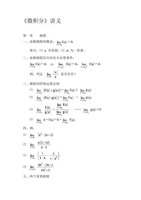
《微积分》讲义第一章极限一、函数极限的概念：f＝A要点：⑴x 为变量；⑵A 为一常量。

二、函数极限存在的充分必要条件：f＝A f＝A，f＝A 例：判定是否存在？三、极限的四则运算法则⑴＝f±g⑵＝f·g⑶＝……g≠0⑷k·f＝k·f四、例：⑴⑵⑶⑷五、两个重要极限⑴＝1 ＝1⑵＝e ＝e ………型理论依据：⑴两边夹法则：若f≤g≤h，且limf＝limh＝A，则：limg＝A⑵单调有界数列必有极限。

例题：⑴＝⑵＝⑶＝⑷＝⑸＝六、无穷小量及其比较1、无穷小量定义：在某个变化过程中趋向于零的变量。

2、无穷大量定义：在某个变化过程中绝对值无限增大的变量。

3、高阶无穷小，低阶无穷小，同阶无穷小，等价无穷小。

4、定理：f＝A f＝A＋a （a＝0）七、函数的连续性1、定义：函数y＝f在点处连续……在点处给自变量x一改变量x：⑴x0时，y0。

即：y＝0⑵f＝f⑶左连续：f＝f右连续：f＝f2、函数y＝f在区间上连续。

3、连续函数的性质：⑴若函数f和g都有在点处连续，则：f±g、f·g、（g()≠0）在点处连续。

⑵若函数u＝j在点处连续，而函数y＝f在点＝j()处连续，则复合函数f(j(x)) 在点处连续。

例：＝＝＝4、函数的间断点：⑴可去间断点：f＝A，但f不存在。

⑵跳跃间断点：f＝A ，f＝B，但A≠B。

⑶无穷间断点：函数在此区间上没有定义。

5、闭区间上连续函数的性质：若函数f在闭区间上连续，则：⑴f在闭区间上必有最大值和最小值。

⑵若f与f异号，则方程f＝0 在内至少有一根。

例：证明方程式－4＋1＝0在区间内至少有一个根。

第二章一元函数微分学一、导数1、函数y＝f在点处导数的定义：x y＝f－f＝A f'＝A ……y'，，。

2、函数y＝f在区间上可导的定义：f'，y'，，。

3、基本初等函数的导数公式：⑴＝0⑵＝n·⑶＝，＝⑷＝·lnɑ，＝⑸＝cosx，＝－sinx＝x，＝－＝secx·tanx，＝－cscx·cotx⑹＝－＝－4、导数的运算：⑴、四则运算法则：＝±＝·g(x)＋f(x)·＝例：求下列函数的导数y＝2－5＋3x－7f(x)＝＋4cosx－siny＝⑵、复合函数的求导法则：y u，u v，v w，w x y x'＝''''例：y＝lntanxy＝lny＝arcsin⑶、隐函数的求导法则：把y看成是x的复合函数，即遇到含有y 的式子，先对y求导，然后y再对x求导。

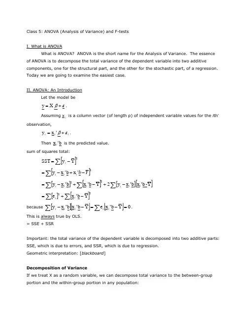
Class 5: ANOVA (Analysis of Variance) and F-testsI. What is ANOVAWhat is ANOVA? ANOVA is the short name for the Analysis of Variance. The essenceof ANOVA is to decompose the total variance of the dependent variable into two additive components, one for the structural part, and the other for the stochastic part, of a regression. Today we are going to examine the easiest case.II. ANOVA: An IntroductionLet the model beεβ+= X y .Assuming x i is a column vector (of length p) of independent variable values for the i th'observation,i i i εβ+='x y .Then b 'x i is the predicted value.sum of squares total:[]∑-=2Y y SST i []∑-+-=2'x b 'x y Y b i i i[][][][]∑∑∑-+-+-=Y -b 'x b 'x y 2Y b 'x b 'x y 22i i i i i i[][]∑∑-+=22Y b 'x e i ibecause [][][]∑∑=-=--0Y b 'x e Y b 'x b 'x y ii i i i .This is always true by OLS. = SSE + SSRImportant: the total variance of the dependent variable is decomposed into two additive parts: SSE, which is due to errors, and SSR, which is due to regression. Geometric interpretation: [blackboard ]Decomposition of VarianceIf we treat X as a random variable, we can decompose total variance to the between-group portion and the within-group portion in any population:()()()i i i x y εβV 'V V +=Prove:()()i i i x y εβ+='V V()()()i i i i x x εβεβ,'Cov 2V 'V ++=()()iix εβV 'V +=(by the assumption that ()0 ,'Cov =εβk x , for all possible k.)The ANOVA table is to estimate the three quantities of equation (1) from the sample.As the sample size gets larger and larger, the ANOVA table will approach the equation closer and closer.In a sample, decomposition of estimated variance is not strictly true. We thus need toseparately decompose sums of squares and degrees of freedom. Is ANOVA a misnomer?III. ANOVA in MatrixI will try to give a simplied representation of ANOVA as follows:[]∑-=2Y y SST i ()∑-+=i i y Y 2Y y 22∑∑∑-+=i i y Y 2Y y 22∑-+=222Y n 2Y n y i (because ∑=Y n y i )∑-=22Y n y i2Y n y 'y -=y J 'y n /1y 'y -= (in your textbook, monster look)SSE = e'e[]∑-=2Y b 'x SSR i()()[]∑-+=Y b 'x 2Y b 'x 22i i()[]()∑∑-+=b 'x Y 2Y n b 'x 22i i()[]()∑∑--+=i i i e y Y 2Y n b 'x 22()[]∑-+=222Y n 2Y n b 'x i(because ∑∑==0e ,Y n y i i , as always)()[]∑-=22Yn b 'x i2Y n Xb X'b'-=y J 'y n /1y X'b'-= (in your textbook, monster look)IV. ANOVA TableLet us use a real example. Assume that we have a regression estimated to be y = - 1.70 + 0.840 xANOVA TableSOURCE SS DF MS F with Regression 6.44 1 6.44 6.44/0.19=33.89 1, 18Error 3.40 18 0.19 Total 9.8419We know∑=100xi, ∑=50y i , 12.509x 2=∑i , 84.134y 2=∑i , ∑=66.257y x i i . If weknow that DF for SST=19, what is n?n= 205.220/50Y ==84.95.25.22084.134Y n y SST 22=⨯⨯-=-=∑i()[]∑-+=0.1250.84x 1.7-SSR 2i[]∑-⨯⨯⨯-⨯+⨯=0.125x 84.07.12x 84.084.07.17.12i i= 20⨯1.7⨯1.7+0.84⨯0.84⨯509.12-2⨯1.7⨯0.84⨯100- 125.0= 6.44SSE = SST-SSR=9.84-6.44=3.40DF (Degrees of freedom): demonstration. Note: discounting the intercept when calculating SST. MS = SS/DFp = 0.000 [ask students]. What does the p-value say?V. F-TestsF-tests are more general than t-tests, t-tests can be seen as a special case of F-tests.If you have difficulty with F-tests, please ask your GSIs to review F-tests in the lab. F-tests takes the form of a fraction of two MS's.MSR/MSE F , df2df1An F statistic has two degrees of freedom associated with it: the degree of freedom inthe numerator, and the degree of freedom in the denominator.An F statistic is usually larger than 1. The interpretation of an F statistics is thatwhether the explained variance by the alternative hypothesis is due to chance. In other words, the null hypothesis is that the explained variance is due to chance, or all the coefficients are zero.The larger an F-statistic, the more likely that the null hypothesis is not true. There is atable in the back of your book from which you can find exact probability values.In our example, the F is 34, which is highly significant.VI. R 2R 2 = SSR / SSTThe proportion of variance explained by the model. In our example, R-sq = 65.4%VII. What happens if we increase more independent variables.1. SST stays the same.2. SSR always increases.3. SSE always decreases.4. R 2 always increases.5. MSR usually increases.6. MSE usually decreases.7. F-test usually increases.Exceptions to 5 and 7: irrelevant variables may not explain the variance but take up degrees of freedom. We really need to look at the results.VIII. Important: General Ways of Hypothesis Testing with F-Statistics.All tests in linear regression can be performed with F-test statistics. The trick is to run"nested models."Two models are nested if the independent variables in one model are a subset or linearcombinations of a subset （子集）of the independent variables in the other model.That is to say. If model A has independent variables (1, 1x , 2x ), and model B hasindependent variables (1, 1x , 2x ,3x ), A and B are nested. A is called the restricted model; B is called less restricted or unrestricted model. We call A restricted because A implies that0=3β. This is a restriction.Another example: C has independent variable (1, 1x , 2x +3x ), D has (1, 2x +3x ). C and A are not nested.C and B are nested. One restriction in C: 32ββ=.C andD are nested. One restriction in D: 0=1β. D and A are not nested.D and B are nested: two restriction in D: 32ββ=; 0=1β.We can always test hypotheses implied in the restricted models. Steps: run tworegression for each hypothesis, one for the restricted model and one for the unrestrictedmodel. The SST should be the same across the two models. What is different is SSE and SSR. That is, what is different is R 2. Let()()df df SSE ,df df SSE u u r r ==;df df ()()0u r u r r u n p n p p p -=---=-<Use the following formulas:()()()()(),SSE SSE /df SSE df SSE F SSE /df r u r u dfr dfu dfu u u---=or()()()()(),SSR SSR /df SSR df SSR F SSE /df u r u r dfr dfu dfu u u---=(proof: use SST = SSE+SSR)Note, df(SSE r )-df(SSE u ) = df(SSR u )-df(SSR r ) =df ∆,is the number of constraints (not number of parameters) implied by the restricted modelor()()()22,2R R /df F 1R /dfur dfr dfu dfuuu--∆=- Note thatdf 1df ,2F t =That is, for 1df tests, you can either do an F-test or a t-test. They yield the same result. Another way to look at it is that the t-test is a special case of the F test, with the numerator DF being 1.IX. Assumptions of F-testsWhat assumptions do we need to make an ANOVA table work?Not much an assumption. All we need is the assumption that (X'X) is not singular, so that the least square estimate b exists.The assumption of ε'X =0 is needed if you want the ANOVA table to be an unbiased estimate of the true ANOVA (equation 1) in the population. Reason: we want b to be an unbiased estimator of β, and the covariance between b and εto disappear.For reasons I discussed earlier, the assumptions of homoscedasticity and non-serial correlation are necessary for the estimation of ()i V ε.The normality assumption that εi is distributed in a normal distribution is needed for small samples.X. The Concept of IncrementEvery time you put one more independent variable into your model, you get an increase in 2R . We sometime called the increase "incremental 2R ." What is means is that more variance is explained, or SSR is increased, SSE is reduced. What you should understand is that the incremental 2R attributed to a variable is always smaller than the 2R when other variables are absent.XI. Consequences of Omitting Relevant Independent VariablesSay the true model is the following:0112233i i i i i y x x x ββββε=++++.But for some reason we only collect or consider data on 21,,x and x y . Therefore, we omit3x in the regression. That is, we omit in 3x our model. We briefly discussed this problembefore. The short story is that we are likely to have a bias due to the omission of a relevant variable in the model. This is so even though our primary interest is to estimate the effect of1x or 2x on y.Why? We will have a formal presentation of this problem.XII. Measures of Goodness-of-FitThere are different ways to assess the goodness-of-fit of a model. A. R 2R 2 is a heuristic measure for the overall goodness-of-fit. It does not have an associated test statistic.R 2 measures the proportion of the variance in the dependent variable that is “explained” by the model: R 2 =SSESSR SSRSST SSR +=B. Model F-testThe model F-test tests the joint hypotheses that all the model coefficients except for the constant term are zero.Degrees of freedoms associated with the model F-test: Numerator: p-1 Denominator: n-p.C. t-tests for individual parametersA t-test for an individual parameter tests the hypothesis that a particular coefficient is equal to a particular number (commonly zero).t k = (b k - βk0)/SE k , where SE k is the (k, k) element of MSE(X’X)-1, with degree of freedom=n-p. D. Incremental R 2Relative to a restricted model, the gain in R 2 for the unrestricted model: ∆R 2= R u 2- R r 2E. F-tests for Nested ModelIt is the most general form of F-tests and t-tests.()()()()(),SSE SSE /df SSE df SSE F SSE /df r u r dfu dfr u dfu u u---=It is equal to a t-test if the unrestricted and restricted models differ only by one single parameter.It is equal to the model F-test if we set the restricted model to the constant-only model.[Ask students] What are SST, SSE, and SSR, and their associated degrees of freedom, for the constant-only model?Numerical ExampleA sociological study is interested in understanding the social determinants of mathematicalachievement among high school students. You are now asked to answer a series of questions. The data are real but have been tailored for educational purposes. The total number of observations is 400. The variables are defined as: y: math scorex1: father's education x2: mother's educationx3: family's socioeconomic status x4: number of siblings x5: class rankx6: parents' total education (note: x6 = x1 + x2) For the following regression models, we know: Table 1 SST SSR SSE DF R 2 (1) y on (1 x1 x2 x3 x4) 34863 4201 (2) y on (1 x6 x3 x4) 34863 396 .1065 (3) y on (1 x6 x3 x4 x5) 34863 10426 24437 395 .2991 (4) x5 on (1 x6 x3 x4) 269753 396 .02101. Please fill the missing cells in Table 1.2. Test the hypothesis that the effects of father's education (x1) and mother's education (x2) on math score are the same after controlling for x3 and x4.3. Test the hypothesis that x6, x3 and x4 in Model (2) all have a zero effect on y.4. Can we add x6 to Model (1)? Briefly explain your answer.5. Test the hypothesis that the effect of class rank (x5) on math score is zero after controlling for x6, x3, and x4.Answer: 1. SST SSR SSE DF R 2 (1) y on (1 x1 x2 x3 x4) 34863 4201 30662 395 .1205 (2) y on (1 x6 x3 x4) 34863 3713 31150 396 .1065 (3) y on (1 x6 x3 x4 x5) 34863 10426 24437 395 .2991 (4) x5 on (1 x6 x3 x4) 275539 5786 269753 396 .0210Note that the SST for Model (4) is different from those for Models (1) through (3). 2.Restricted model is 01123344()y b b x x b x b x e =+++++Unrestricted model is ''''''011223344y b b x b x b x b x e =+++++(31150 - 30662)/1F 1,395 = -------------------- = 488/77.63 = 6.29 30662 / 395 3.3713 / 3F 3,396 = --------------- = 1237.67 / 78.66 = 15.73 31150 / 3964. No. x6 is a linear combination of x1 and x2. X'X is singular.5.(31150 - 24437)/1F 1,395 = -------------------- = 6713 / 61.87 = 108.50 24437/395t = 10.42t ===。

第二章导数与微分第一节导数概念一、导数的定义 定义：若极限()()lim lim 0000x x f x x f x y x x∆→∆→+∆-∆=∆∆存在，则称函数()y f x =在点0x 处可导，此极限值称为函数()y f x =在点0x 处的导数。

记为： ()0f x '、0x x y ='、0x x dy dx =、()0x x df x dx = （或极限()()lim 000x x f x f x x x →--存在也可）()()lim lim 0000x x f x x f x y x x∆→∆→+∆-∆=∆∆单侧导数：左导数：()()lim 000x f x x f x x-∆→+∆-=∆()()lim 000x x f x f x x x -→--存在，则称左导数存在，记为：()0f x -'。

右导数：()()lim 000x f x x f x x+∆→+∆-=∆()()lim 000x x f x f x x x +→--存在，则称右导数存在，记为：()0f x +'。

【例1】（89一）已知()32f '=，则【例2】（87二）设()f x 在x a =处可导，则（A ）()f a '. （B ）()2f a '.（C ）0. （D ）()2f a '.【例3】（89二）设()()()()12f x x x x x n =+++，则()0f '= .（C）可导，但导数不连续. （D）可导，但导数连续.处的（A）左、右导数都存在. （B）左导数存在，但右导数不存在.（C）左导数不存在，但右导数存在.（D）左、右导数都不存在.【例7】（96二）设函数()f x在区间(,)-δδ内有定是()f x的（A）间断点. （B）连续而不可导的点. （C）可导的点，且()00f'=.（D）可导的点，且()00f'≠.【例8】（90三）设函数()f x 对任意的x 均满足等式()()1f x af x +=，且有()0f b '=，其中a 、b 为非零常数，则（A ）()f x 在1x =处不可导.（B ）()f x 在1x =处可导，且()1f a '=.（C ）()f x 在1x =处可导，且()1f b '=.（D ）()f x 在1x =处可导，()1f ab '=.二、导数的几何意义和物理意义导数的几何意义： 切线的斜率为：()()tan lim 00x x f x f x k x x →-==-α， ()()00f x f x x x --导数的物理意义：某变量对时间t 的变化率，常见的有速度和加速度。

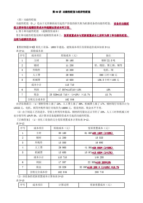
第05讲功能性贬值与经济性贬值（四）功能性贬值功能性贬值（D f）是由于无形磨损而引起资产价值的损失称为机器设备的功能性贬值。

设备的功能贬值主要体现在超额投资成本和超额运营成本两方面。

1.第Ⅰ种功能性贬值（超额投资成本）第I种功能性贬值反映在超额投资成本上，复原重置成本与更新重置成本之差即为第I种功能性贬值，也称为超额投资成本。

【教材例题3-9】某化工设备，1980年建造，建筑成本项目及原始造价成本如表3-11表3-11 原始成本表在评估基准日:（1）钢材价格上涨了23%，人工费上涨了39%，机械费上涨了17%，辅材现行市场合计为13328元，电机、阀等外购件现行市场价为16698元，假设利润、税金水平不变。

（2）由于制造工艺的进步，导致主材利用率提高，钢材的用量比过去节约了20%，人工工时和机械工时也分别节约15%和8%。

试计算该设备超额投资成本引起的功能性贬值。

『正确答案』（1）该化工设备的完全复原重置成本计算如表3-12。

表3-12（2）该设备的更新重置成本计算如表3-13表3-13（3）超额投资成本引起的功能性贬值超额投资成本引起的功能性贬值=复原重置成本-更新重置成本=203 740-176 641=27 099（元）2.第Ⅱ种功能性贬值（运营性功能性贬值）计算超额运营成本引起的功能性贬值的步骤如下：（1）分析比较被评估机器设备的超额运营成本因素；（2）确定被评估设备的尚可使用寿命，计算每年的超额运营成本；（3）计算净超额运营成本；（4）确定折现率，计算超额运营成本的折现值。

【教材例题3-10】计算某电焊机超额运营成本引起的功能性贬值。

（1）分析比较被评估机器设备的超额运营成本因素：经分析比较，被评估的电焊机与新型电焊机相比，引起超额运营成本的因素主要为老产品的能耗比新产品高。

通过统计分析，按每天8小时工作，每年300个工作日，每台老电焊机比新电焊机多耗电6000度。

（2）确定被评估设备的尚可使用寿命，计算每年的超额运营成本：根据设备的现状，评估人员预计该电焊机尚可使用10年，如每度电按0.5元计算，则：每年的超额运营成本=6000 ×0.5 =3 000（元）（3）计算净超额运营成本：所得税按25%计算，则：税后每年净超额运营成本=税前超额运营成本×（1-所得税）=3000×（1-25%）=2 250（元）（4）确定折现率，计算超额运营成本的折现值：折现率为10%，10年的年金现值系数为6.145，则：净超额运营成本的折现值=净超额运营成本×年金折现系数＝2 250×6.145≈13 826（元）该电焊机由于超额运营成本引起的功能性贬值为13 826元。

D/F培训讲义一．D/F目的：将线路图形转移到铜面上二．D/F流程：磨板→贴膜→曝光→显影三．各工序特点1．前处理：a.目的：除氧化，粗化铜b.主要参数：磨痕宽度，磨刷速度，酸液浓度，水膜试验c.常见问题：（1）板面星点氧化：风刀堵塞或风管破损漏风或鼓风机故障（2）板面光泽差：砂粉浓度低（3）板面有砂粉：砂粉粒径过大，水流压力偏小2．贴膜：a.目的：贴覆干膜，在板上形成抗蚀剂层b.主要参数：贴膜压力，贴膜速度，贴膜温度c.常见问题：（1）粘贴不牢：干膜储存时间过久，覆铜箔板清洁处理不良，环境湿度太低, 贴膜温度过低或传送速度太快。

（2）气泡：贴膜温度过高，热压辊表面不平有凹坑或划伤, 压辊压力太小, 板面不平有划痕或凹坑。

（3）干膜起皱：两个热压辊轴向不平行，贴膜温度太高, 贴膜前板子太热。

3．曝光：a.目的：对干膜进行光固化b.主要参数：曝光尺，真空度c.常见问题：（1）曝光垃圾：清洁度不够。

（2）曝光不良：真空度不足，菲林光密度不足，未擦气或曝光时菲林药膜贴反4．冲板a.目的：将曝光之干膜留于板面，未曝光之干膜去除b.主要参数：显影速度，显影温度，显影压力，药水浓度c.常见问题：（1）显影不净：显影速度过快，药水温度偏低，压力偏低，浓度偏低（2）显影过度：显影速度过慢，药水温度偏高，压力偏大，浓度偏高（3）菲林碎：显影液过滤不好，水洗压力偏大。

四．常见问题及解决方法：在使用干膜进行图像转移时，由于干膜本身的缺陷或操作工艺不当，可能会出现各种质量问题。

下面列举在生产过程中可能产生的故障，并分析原因，提出排除故障的方法。

2＞干膜与铜箔表面之间出现气泡5＞显影后干膜图像模糊，抗蚀剂发暗发毛。

力士乐A10V S O-D F L R 变量泵的控制原理档
力士乐Ａ１０ＶＳＯ－ＤＦＬＲ（恒压/流量/功率控制）变量泵的控制原理
我的问题已经提出好几天了．无人回帖．可能是我对问题的叙述不很清楚．最近几天我琢磨了一下，对于功率阀的调节原理,我先试着分析如下.是我个人的理解,请诸位指正.
功率阀相当于一个压力无级可调的(比例)溢流阀,它可无级地改变着进入流量调节器弹簧腔的压力P H.压力的无级可调是通过泵斜盘改变功率阀调压弹簧的压缩量X来实现的(泵斜盘带动拨杆改变功率阀套的位置,进而改变功率阀调压弹簧的压缩量X), 压缩量X与泵斜盘倾角β成反比.
在泵进入恒功率控制期间,流量调节器控制阀芯的位置也有3个.
压力P H作用在控制阀芯的右端(见图1),以形成一个对抗反力,与作用在控制阀芯左端的泵出口压力P P相平衡,使控制阀芯保持在中位(平衡位置),在此状态下,泵的斜盘倾角不变.
功率阀所决定的压力P H与泵压力P P应该是同比例变化(升降)的.并且P H的变化要比P P的变化滞后一点时间.
当泵压升高时,P P先将控制阀芯向右推离中位(平衡被破坏),并进入泵变量缸的无杆腔使泵的斜盘倾角β变小(流量减小), 随着倾角β的变小,功率阀调压弹簧的压缩量X则变大,阀的开启压力P H随之升高,升高了的P H又将控制阀芯推回中位恢复平衡状态.如此循环下去,控制阀芯连续的经历由平衡→不平衡→新的平衡的过程(用一位网友的话讲,就是控制阀芯在“中位振荡”),便实现了恒功率控制.
当泵压降低时,则会出现相反的过程.
恒功率控制始于起点的调整压力，终于切断点的限位柱（即死档铁）．不知我分析的对不对，请各位点拨．。

DF4课程设计一、课程目标知识目标：1. 让学生掌握DF4型内燃机车的构造原理，理解其工作过程及主要部件的功能。

2. 使学生了解我国铁路运输中DF4型内燃机车的应用及发展，掌握相关铁路知识。

技能目标：1. 培养学生运用课本知识，分析DF4型内燃机车故障原因及维修方法的能力。

2. 提高学生实际操作能力，学会使用相关工具对DF4型内燃机车进行简单维护。

情感态度价值观目标：1. 培养学生对铁路事业的热爱，增强对我国铁路发展的信心。

2. 培养学生团队合作精神，提高解决实际问题的能力。

3. 增强学生环保意识，了解内燃机车在环保方面的优势与不足。

课程性质分析：本课程为铁路运输专业课程，以DF4型内燃机车为主要教学内容，注重理论与实践相结合，培养学生的实际操作能力。

学生特点分析：学生为铁路运输专业中职二年级学生，具备一定的铁路基础知识，对内燃机车有一定了解，动手能力强，对实际操作感兴趣。

教学要求：1. 结合课本知识，深入浅出地讲解DF4型内燃机车的构造、原理及维修方法。

2. 采取案例教学，提高学生分析问题和解决问题的能力。

3. 加强实践教学，让学生在实际操作中掌握技能，培养团队合作精神。

二、教学内容1. DF4型内燃机车概述：介绍DF4型内燃机车的背景、发展历程、主要性能参数及其在铁路运输中的应用。

教材章节：《内燃机车概论》第二章第二节2. DF4型内燃机车构造：详细讲解DF4型内燃机车的车体结构、动力装置、传动装置、走行装置等主要部件及其功能。

教材章节：《内燃机车构造》第三章3. DF4型内燃机车工作原理：分析DF4型内燃机车的启动、运行、制动等过程，阐述各部件协同工作的原理。

教材章节：《内燃机车工作原理》第四章4. DF4型内燃机车维护与故障处理：结合实际案例，讲解DF4型内燃机车的日常维护、检查方法以及常见故障的处理技巧。

教材章节：《内燃机车维护与故障处理》第五章5. 实践教学：安排学生进行DF4型内燃机车的现场观察、简单维护操作和模拟故障排除，提高学生的实际操作能力。