卡尔曼滤波器介绍外文翻译

卡尔曼滤波是一种高效率的递归滤波器(自回归滤波器), 它能够从一系列的不完全包含噪声的测量(英文:measurement)中，估计动态系统的状态。

应用实例卡尔曼滤波的一个典型实例是从一组有限的，对物体位置的，包含噪声的观察序列预测出物体的坐标位置及速度. 在很多工程应用(雷达, 计算机视觉)中都可以找到它的身影. 同时，卡尔曼滤波也是控制理论以及控制系统工程中的一个重要话题.比如,在雷达中,人们感兴趣的是跟踪目标,但目标的位置,速度,加速度的测量值往往在任何时候都有噪声.卡尔曼滤波利用目标的动态信息,设法去掉噪声的影响,得到一个关于目标位置的好的估计。

这个估计可以是对当前目标位置的估计(滤波),也可以是对于将来位置的估计(预测)，也可以是对过去位置的估计(插值或平滑).命名这种滤波方法以它的发明者鲁道夫.E.卡尔曼（Rudolf E. Kalman）命名. 虽然Peter Swerling实际上更早提出了一种类似的算法.斯坦利.施密特(Stanley Schmidt)首次实现了卡尔曼滤波器.卡尔曼在NASA埃姆斯研究中心访问时,发现他的方法对于解决阿波罗计划的轨道预测很有用,后来阿波罗飞船的导航电脑使用了这种滤波器. 关于这种滤波器的论文由Swerling (1958), Kalman (1960)与 Kalman and Bucy (1961)发表.目前,卡尔曼滤波已经有很多不同的实现.卡尔曼最初提出的形式现在一般称为简单卡尔曼滤波器.除此以外,还有施密特扩展滤波器,信息滤波器以及很多Bierman, Thornton 开发的平方根滤波器的变种.也行最常见的卡尔曼滤波器是锁相环，它在收音机,计算机和几乎任何视频或通讯设备中广泛存在.欧阳光明（2021.03.07）卡尔曼滤波器– Kalman Filter1．什么是卡尔曼滤波器（What is the Kalman Filter ）在学习卡尔曼滤波器之前，首先看看为什么叫“卡尔曼”。

卡尔曼滤波是一种高效率的递归滤波器(自回归滤波器), 它能够从一系列的不完全包含噪声的测量(英文:measurement)中，估计动态系统的状态。

应用实例卡尔曼滤波的一个典型实例是从一组有限的，对物体位置的，包含噪声的观察序列预测出物体的坐标位置及速度. 在很多工程应用(雷达, 计算机视觉)中都可以找到它的身影. 同时，卡尔曼滤波也是控制理论以及控制系统工程中的一个重要话题.比如,在雷达中,人们感兴趣的是跟踪目标,但目标的位置,速度,加速度的测量值往往在任何时候都有噪声.卡尔曼滤波利用目标的动态信息,设法去掉噪声的影响,得到一个关于目标位置的好的估计。

这个估计可以是对当前目标位置的估计(滤波),也可以是对于将来位置的估计(预测)，也可以是对过去位置的估计(插值或平滑).命名这种滤波方法以它的发明者鲁道夫.E.卡尔曼（Rud olf E. Kalman）命名. 虽然Peter Swerling实际上更早提出了一种类似的算法.斯坦利.施密特(Stanley Schmidt)首次实现了卡尔曼滤波器.卡尔曼在NASA埃姆斯研究中心访问时,发现他的方法对于解决阿波罗计划的轨道预测很有用,后来阿波罗飞船的导航电脑使用了这种滤波器.关于这种滤波器的论文由Swerling (1958), Kalm an (1960)与 Kalman and Bucy (1961)发表.目前,卡尔曼滤波已经有很多不同的实现.卡尔曼最初提出的形式现在一般称为简单卡尔曼滤波器.除此以外,还有施密特扩展滤波器,信息滤波器以及很多Bierman, Thornton 开发的平方根滤波器的变种.也行最常见的卡尔曼滤波器是锁相环，它在收音机,计算机和几乎任何视频或通讯设备中广泛存在.卡尔曼滤波器– Kalman Filter1．什么是卡尔曼滤波器（What is the Kalman Filter ）在学习卡尔曼滤波器之前，首先看看为什么叫“卡尔曼”。

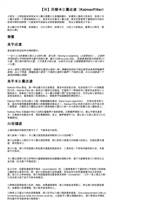
【译】图解卡尔曼滤波（KalmanFilter）译者注：这恐怕是全网有关卡尔曼滤波最简单易懂的解释，如果你认真的读完本文，你将对卡尔曼滤波有一个更加清晰的认识，并且可以手推卡尔曼滤波。

原文作者使用了漂亮的图片和颜色来阐明它的原理（读起来并不会因公式多而感到枯燥），所以请勇敢地读下去！本人翻译水平有限，如有疑问，请阅读原文；如有错误，请在评论区指出。

推荐阅读原文，排版比较美:)背景关于滤波首先援引来自知乎大神的解释。

“一位专业课的教授给我们上课的时候，曾谈到：filtering is weighting（滤波即加权）。

滤波的作用就是给不同的信号分量不同的权重。

最简单的loss pass filter，就是直接把低频的信号给1权重，而给高频部分0权重。

对于更复杂的滤波，比如维纳滤波, 则要根据信号的统计知识来设计权重。

从统计信号处理的角度，降噪可以看成滤波的一种。

降噪的目的在于突出信号本身而抑制噪声影响。

从这个角度，降噪就是给信号一个高的权重而给噪声一个低的权重。

维纳滤波就是一个典型的降噪滤波器。

”关于卡尔曼滤波Kalman Filter 算法，是一种递推预测滤波算法，算法中涉及到滤波，也涉及到对下一时刻数据的预测。

Kalman Filter 由一系列递归数学公式描述。

它提供了一种高效可计算的方法来估计过程的状态，并使估计均方误差最小。

卡尔曼滤波器应用广泛且功能强大：它可以估计信号的过去和当前状态，甚至能估计将来的状态，即使并不知道模型的确切性质。

Kalman Filter 也可以被认为是一种数据融合算法（Data fusion algorithm），已有50多年的历史，是当今使用最重要和最常见的数据融合算法之一。

Kalman Filter 的巨大成功归功于其小的计算需求，优雅的递归属性以及作为具有高斯误差统计的一维线性系统的最优估计器的状态。

Kalman Filter 只能减小均值为0的测量噪声带来的影响。

卡尔曼滤波英文版The Kalman Filter: A Powerful Tool for Optimal Estimation and PredictionThe Kalman filter is a mathematical algorithm that provides an efficient computational means to estimate the state of a dynamic system from a series of measurements. Developed by Rudolf E. Kalman in 1960, this powerful tool has found widespread applications in various fields, including aerospace engineering, robotics, navigation, and signal processing. The Kalman filter is particularly useful in situations where the system being observed is subject to random disturbances or the measurements contain noise.At the heart of the Kalman filter is the concept of state estimation. In a dynamic system, the state represents the essential information needed to describe the system's behavior at a particular point in time. This state may include variables such as position, velocity, acceleration, or any other relevant parameters. The Kalman filter uses a recursive algorithm to estimate the system's state based on a series of noisy measurements, providing an optimal estimate thatminimizes the mean square error.The Kalman filter operates in two distinct phases: the prediction phase and the update phase. In the prediction phase, the algorithm uses the system's dynamics and the previous state estimate to predict the current state. This prediction is then combined with the current measurement in the update phase, where the Kalman filter calculates a weighted average of the predicted state and the measured state. The weighting factor, known as the Kalman gain, is determined based on the relative uncertainties of the prediction and the measurement.One of the key advantages of the Kalman filter is its ability to handle uncertainty and noise in the system and measurements. By continuously updating the state estimate based on the available measurements, the Kalman filter can effectively filter out the noise and provide a smooth, accurate estimate of the system's state. This makes the Kalman filter particularly useful in applications where the measurements are unreliable or subject to various sources of noise, such as sensor errors, environmental disturbances, or measurement delays.Another important aspect of the Kalman filter is its recursive nature. Instead of storing and processing all past measurements, the Kalman filter only requires the current measurement and the previous stateestimate to compute the current state estimate. This makes the algorithm computationally efficient and well-suited for real-time applications, where the system's state needs to be estimated and updated continuously.The versatility of the Kalman filter has led to its widespread adoption in a variety of applications. In the field of aerospace engineering, the Kalman filter is extensively used for aircraft and spacecraft navigation, guidance, and control. By combining measurements from multiple sensors, such as GPS, inertial measurement units, and radar, the Kalman filter can provide a robust and accurate estimate of the vehicle's position, orientation, and velocity.In the field of robotics, the Kalman filter is used to track the position and orientation of mobile robots, enabling them to navigate through complex environments and perform tasks with high precision. In signal processing, the Kalman filter is employed to remove noise and distortion from various types of signals, such as audio, video, and communication signals, improving the quality and clarity of the output.Beyond these traditional applications, the Kalman filter has also found use in emerging areas like autonomous vehicles, where it plays a crucial role in fusing data from multiple sensors (e.g., cameras, lidar, radar) to provide a comprehensive understanding of the vehicle'ssurroundings and enable accurate localization, mapping, and decision-making.The widespread adoption of the Kalman filter is a testament to its mathematical elegance and practical effectiveness. The algorithm's ability to provide optimal state estimates in the presence of uncertainty and noise has made it an indispensable tool in a wide range of fields, from aerospace to robotics and beyond.As technology continues to advance, the Kalman filter is likely to remain a fundamental component in many complex systems, enabling more accurate, reliable, and efficient solutions to a myriad of real-world problems. Its ongoing evolution and integration with emerging technologies, such as deep learning and sensor fusion, are likely to unlock even greater capabilities and applications in the years to come.。

卡尔曼滤波卡尔曼滤波(Kalman filtering ) 一种利用线性系统状态方程，通过系统输入输出观测数据，对系统状态进行最优估计的算法。

由于观测数据中包括系统中的噪声和干扰的影响，所以最优估计也可看作是滤波过程。

斯坦利施密特(Stanley Schmidt)首次实现了卡尔曼滤波器。

卡尔曼在NASA埃姆斯研究中心访问时，发现他的方法对于解决阿波罗计划的轨道预测很有用，后来阿波罗飞船的导航电脑使用了这种滤波器。

关于这种滤波器的论文由Swerli ng (1958), Kalman (I960) 与Kalma n and Bucy (1961) 发表。

数据滤波是去除噪声还原真实数据的一种数据处理技术，Kalman滤波在测量方差已知的情况下能够从一系列存在测量噪声的数据中，估计动态系统的状态•由于，它便于计算机编程实现，并能够对现场采集的数据进行实时的更新和处理，Kalman滤波是目前应用最为广泛的滤波方法，在通信，导航，制导与控制等多领域得到了较好的应用•中文名卡尔曼滤波器，Kalman滤波，卡曼滤波外文名KALMAN FILTER表达式X(k)=A X(k-1)+B U(k)+W(k)提岀者斯坦利施密特提岀时间1958应用学科天文，宇航，气象适用领域范围雷达跟踪去噪声适用领域范围控制、制导、导航、通讯等现代工程斯坦利施密特(Stanley Schmidt)首次实现了卡尔曼滤波器。

卡尔曼在NASA埃姆斯研究中心访问时，发现他的方法对于解决阿波罗计划的轨道预测很有用，后来阿波罗飞船的导—航电脑使用了这种滤波器。

关于这种滤波器的论文由Swerling (1958)， Kalman (1960)与Kalma n and Bucy (1961) 发表。

2定义传统的滤波方法，只能是在有用信号与噪声具有不同频带的条件下才能实现. 20世纪40年代，N .维纳和A. H .柯尔莫哥罗夫把信号和噪声的统计性质引进了滤波理论，在假设信号和噪声都是平稳过程的条件下，利用最优化方法对信号真值进行估计，达到滤波目的，从而在概念上与传统的滤波方法联系起来，被称为维纳滤波。

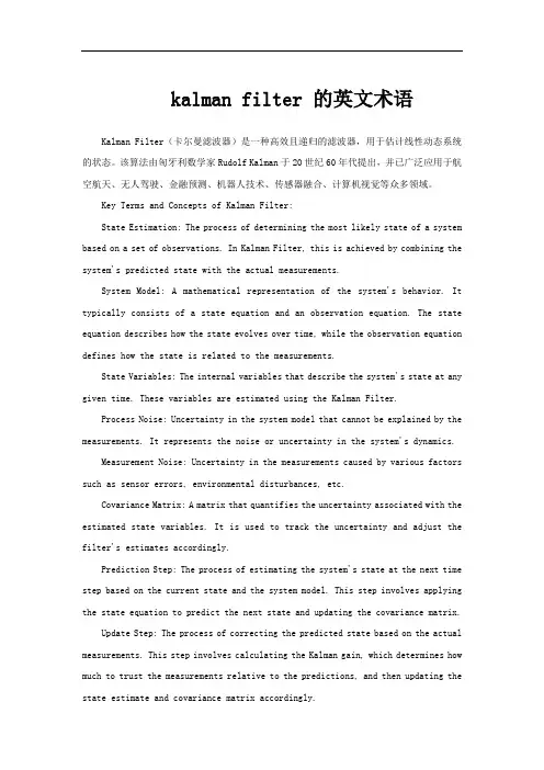
kalman filter 的英文术语Kalman Filter（卡尔曼滤波器）是一种高效且递归的滤波器，用于估计线性动态系统的状态。

该算法由匈牙利数学家Rudolf Kalman于20世纪60年代提出，并已广泛应用于航空航天、无人驾驶、金融预测、机器人技术、传感器融合、计算机视觉等众多领域。

Key Terms and Concepts of Kalman Filter:State Estimation: The process of determining the most likely state of a system based on a set of observations. In Kalman Filter, this is achieved by combining the system's predicted state with the actual measurements.System Model: A mathematical representation of the system's behavior. It typically consists of a state equation and an observation equation. The state equation describes how the state evolves over time, while the observation equation defines how the state is related to the measurements.State Variables: The internal variables that describe the system's state at any given time. These variables are estimated using the Kalman Filter.Process Noise: Uncertainty in the system model that cannot be explained by the measurements. It represents the noise or uncertainty in the system's dynamics.Measurement Noise: Uncertainty in the measurements caused by various factors such as sensor errors, environmental disturbances, etc.Covariance Matrix: A matrix that quantifies the uncertainty associated with the estimated state variables. It is used to track the uncertainty and adjust the filter's estimates accordingly.Prediction Step: The process of estimating the system's state at the next time step based on the current state and the system model. This step involves applying the state equation to predict the next state and updating the covariance matrix.Update Step: The process of correcting the predicted state based on the actual measurements. This step involves calculating the Kalman gain, which determines how much to trust the measurements relative to the predictions, and then updating the state estimate and covariance matrix accordingly.The Kalman Filter algorithm iterates between these prediction and update steps, continuously improving the state estimation as new measurements become available. Its recursive nature allows it to process data in real-time, making it an ideal choice for many real-world applications.。

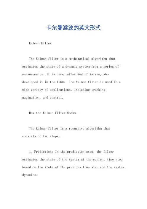
卡尔曼滤波的英文形式Kalman Filter.The Kalman filter is a mathematical algorithm that estimates the state of a dynamic system from a series of measurements. It is named after Rudolf Kalman, who developed it in the 1960s. The Kalman filter is used in a wide variety of applications, including tracking, navigation, and control.How the Kalman Filter Works.The Kalman filter is a recursive algorithm that consists of two steps:1. Prediction: In the prediction step, the filter estimates the state of the system at the current time step based on the state at the previous time step and the system dynamics.2. Update: In the update step, the filter updates the estimate of the state based on the new measurement.The Kalman filter is a powerful tool for estimating the state of a dynamic system. However, it is important to note that the filter is only as good as the model of the system that is used. If the model is not accurate, then the filter will not be able to provide accurate estimates.Applications of the Kalman Filter.The Kalman filter is used in a wide variety of applications, including:Tracking: The Kalman filter can be used to track the position and velocity of a moving object. This is usefulfor applications such as tracking satellites, aircraft, and missiles.Navigation: The Kalman filter can be used to navigate a vehicle by combining measurements from a variety of sensors, such as GPS, accelerometers, and gyroscopes.Control: The Kalman filter can be used to control a system by estimating the state of the system and then using that estimate to calculate the appropriate control inputs. This is useful for applications such as controlling robots and self-driving cars.Advantages of the Kalman Filter.The Kalman filter has several advantages over other estimation methods, including:Optimality: The Kalman filter is the optimal estimator for a linear system with Gaussian noise. This means that the filter will provide the most accurate estimates possible given the available measurements.Recursion: The Kalman filter is a recursive algorithm, which means that it can be implemented in real time. Thisis important for applications where it is necessary to estimate the state of a system in a timely manner.Robustness: The Kalman filter is robust to noise and outliers. This means that the filter can still provide accurate estimates even when the measurements are noisy or contain outliers.Disadvantages of the Kalman Filter.The Kalman filter also has some disadvantages, including:Computational complexity: The Kalman filter can be computationally complex, especially for large systems. This can be a problem for applications where real-time estimation is required.Sensitivity to model errors: The Kalman filter is sensitive to errors in the model of the system. This means that the filter can provide inaccurate estimates if the model is not accurate.Initialization: The Kalman filter requires an initial estimate of the state of the system. This estimate can bedifficult to obtain, especially for complex systems.Conclusion.The Kalman filter is a powerful tool for estimating the state of a dynamic system. The filter is optimal for linear systems with Gaussian noise and is recursive, robust, and computationally efficient. However, the filter is also sensitive to model errors and requires an initial estimate of the state of the system.。

Apollo Recognition 是百度Apollo 自动驾驶平台中的一个重要模块，用于实现车辆的感知、识别和预测功能。

卡尔曼滤波（Kalman Filter）是一种常用的状态估计算法，可以用于处理具有噪声的数据。

在Apollo Recognition 中，卡尔曼滤波被用于提高物体检测和跟踪的准确性。

卡尔曼滤波的基本思想是通过观测值来估计系统的状态。

它包括两个步骤：预测和更新。

预测步骤根据系统的动态模型来预测下一时刻的状态和协方差；更新步骤根据观测值来修正预测的状态和协方差。

通过不断迭代这两个步骤，卡尔曼滤波可以逐步逼近系统的真实状态。

在Apollo Recognition 中，卡尔曼滤波主要用于以下几个方面：
1. 目标跟踪：通过卡尔曼滤波对目标的位置、速度等状态进行估计，从而实现对目标的实时跟踪。

2. 传感器融合：将不同类型传感器（如雷达、摄像头等）的数据进行融合，提高目标检测和跟踪的准确性。

3. 运动状态估计：通过对车辆的运动状态进行估计，实现对车辆的控制和规划。

4. 障碍物预测：通过对障碍物的运动状态进行估计，实现对障碍物的预测和避障策略的制定。

通俗解释简单来说，卡尔曼滤波器是一个“optimal recursive data processing algorithm（最优化自回归数据处理算法）”。

对于解决很大部分的问题，他是最优，效率最高甚至是最有用的。

他的广泛应用已经超过30年，包括机器人导航，控制，传感器数据融合甚至在军事方面的雷达系统以及导弹追踪等等。

近年来更被应用于计算机图像处理，例如头脸识别，图像分割，图像边缘检测等等。

卡尔曼滤波器的介绍：为了可以更加容易的理解卡尔曼滤波器，这里会应用形象的描述方法来讲解，而不是像大多数参考书那样罗列一大堆的数学公式和数学符号。

但是，他的5条公式是其核心内容。

结合现代的计算机，其实卡尔曼的程序相当的简单，只要你理解了他的那5条公式。

在介绍他的5条公式之前，先让我们来根据下面的例子一步一步的探索。

假设我们要研究的对象是一个房间的温度。

根据你的经验判断，这个房间的温度是恒定的，也就是下一分钟的温度等于现在这一分钟的温度（假设我们用一分钟来做时间单位）。

假设你对你的经验不是100%的相信，可能会有上下偏差几度。

我们把这些偏差看成是高斯白噪声（White Gaussian Noise），也就是这些偏差跟前后时间是没有关系的而且符合高斯分布（Gaussian Distribution）。

另外，我们在房间里放一个温度计，但是这个温度计也不准确的，测量值会比实际值偏差。

我们也把这些偏差看成是高斯白噪声。

好了，现在对于某一分钟我们有两个有关于该房间的温度值：你根据经验的预测值（系统的预测值）和温度计的值（测量值）。

下面我们要用这两个值结合他们各自的噪声来估算出房间的实际温度值。

假如我们要估算k时刻的是实际温度值。

首先你要根据k-1时刻的温度值，来预测k时刻的温度。

因为你相信温度是恒定的，所以你会得到k时刻的温度预测值是跟k-1时刻一样的，假设是23度，同时该值的高斯噪声的偏差是5度（5是这样得到的：如果k-1时刻估算出的最优温度值的偏差是3，你对自己预测的不确定度是4度，他们平方相加再开方，就是5）。

Filtre de KalmanBerrada Mohamed∗October18,2006Modèle linèaireLe Filtre de Kalman est une approche statistique,d'assimilation de données,dont le principe est de corriger la trajectoir du modèle en combinant les observations avec l'information fournie par le modèle de façonàminimiser l'erreur entre l'état vrai et l'état ltré.Considérons la représentation stochastique de l'espace d'état suivante:X k+1=M k X k+B k u k+G k W kavec M k est la dynamique linéaire,u k est le terme de forçage(tension du vent,..)projetésur les variables par la matrice B k et G k est la matrice d'entrée de bruit W k qui est un bruit Gaussien de moyenne zero et de matrice de covariance Q k et qui modélise l'erreur modèle,L'observation Z k est reliéeàl'état du modèle(inconnu)X k par la relation,diteéquation d'observations, suivanteZ k=H k X k+V kavec H k est un opérateur linéaire d'observation et V k represente l'erreur sur les observations produit par un bruit Gaussien de moyenne nulle et de matrice de covariance R k.L'état initial X0est supposéêtre Gaussien avec une moyenne X0est une matrice de covariance P0.A n d'obtenir l'état optimale du système on doit combiner les observations Z k avec l'information fournie par le modèle X k.Pour résoudre ce problème de trage on doit determiner la densitéde probabilitécondition-nelle de l'état X k sachant l'historique des mesures pris Z1,...,Z l(on note k/l).Cette densitéde probabilitéest Gaussienne(puisqu'on est dans un cas linéaire)et donc complétement caractériser par sa moyenne X k/l et sa matrice de covariance P k/lL'algorithme:•Initialisation de l'état du système et de sa matrice de covarianceX0/0=X0P0/0=P0•Calcul de l'estimation X k/k−1de l'état du systèmeàl'instant kàpartir des mesures disponiblesàl'instant k−1X k/k−1=M k X k−1/k−1+B k u k•Miseàjour intermédiaire de la matrice de covariance de l'état en tenant compte de l'évolution prévue par l'équation d'évolution de l'étatP k/k−1=M k P k−1/k−1M T k+G k Q k G T k∗universitéde Pierre et Marie Curie LOCEAN-IPSL mblod@locean-ipsl.upmc.fr1•Calcul du gain du ltre optimal(qui peutêtre calculéa priori)K k=P k/k−1H T kH k P k/k−1H T k+R k−1•Miseàjour de la matrice de covariance de l'étatP k/k=(I−K k H k)P k/k−1•Réactualisation de l'estimation de l'étatX k/k=X k/k−1+K kZ k−H k X k/k−1Le gain optimal(de Kalman)tient compte des caractéristiques statistiques du bruit de mesure mais ne dépend pas des données mesurées donc il peutêtre calculéa priori.Le cas d'un processus stationnaire représentédans l'espace d'état par leséquations suivantes:X k+1=M X k+B u k+G W ketZ k=H X k+V kModèle non-linèaireLe ltre de Kalman etenduDans le cas non-linèaire la densitéde probabilitéconditionnelle n'est pas Gaussienne.Pour comprendre le linearisation on considère l'exemple simli e suivant:X k+1=M(X k,k)+B k u k+G k W kavec M est la dynamique non linéaire.On considère que l'équation d'observation est linéaire:Z k=H k X k+V kSupposons qu'il est possible de générer un trajectoir de référence x k.On peut doncécrir le système: X k+1=(M(X k,k)−M(x k,k))+M(x k,k)+B k u k+G k W kSi la distance entre x k et l'état réel X k est su sament petite alors il est possible de faire une approximation du système linéaire en utilisant le developpement en séries de TaylorM(X k,k)−M(x k,k)≈M k(X k−x k)avec(M k)i,j=∂(M k(x k,k))i∂(x k)jdoncX k+1=M k X k−M k x k+f(x k,k)+B k u k+G k W k ce qui peut s'écrire:X k+1=M k X k+¯u k+G k W k2avec ¯u k =−M k x k +M (x k ,k )+B k u kLe choix,le plus simple,de la trajectoir de référence x k est le suivant:x k +1=M (x k ,k )+B k u k ,x 0=X 0Le ltre de Kalman etendu:x k +1=M (x k ,k )+B k u k ,x k =X k/kSupposons un cas plus générale :X k +1=f (X k ,u k +1,W k +1)avec une équation d'observation nonlinéaire:Z k =h (X k ,V k )On fait donc une linearisation desfonctions non linéaires:F k =∂f ∂X X k −1|k −1,u k etH k =∂h ∂x ˆx k |k −1et on donne l'algorithme du ltrede Kalman etendu:•La prédictionX k/k −1=f (X k −1/k −1,u k ,0)P k/k −1=F k P k −1/k −1F T k +G k Q k G T k •Calcul du gain du ltre optimal(qui peut être calculéa priori)K k =P k/k −1H T k H k P k/k −1H T k +R k −1•Mise àjour de la matrice decovariance de l'état P k/k =(I −K k H k )P k/k −1•Réactualisation de l'estimationde l'état X k/k =X k/k −1+K k Z k −H k X k/k −1 Le ltre de Kalman d'ensembleLe ltre de Kalman d'ensemble est basésur une représentation de la densitéde probabiltéde l'état estimé,par un nombre ni N d'états de systèmegénéréaleatoirement ξi k −1/k −1,i =1,..,N avec X k −1/k −1=1N Ni =1ξik −1/k −13On introduit la matrice L dite square root matrixL k−1/k−1=ξ1k−1/k−1−X k−1/k−1...ξNk−1/k−1−X k−1/k−1TCette matrice dé nie une approximation de rang N de la matrice de covariance P k−1/k−1:P Nk−1/k−1=1N−1L k−1/k−1L Tk−1/k−1Algorithme:•Miseàjour de la variable aleatoirξik/k−1=f(ξik−1/k−1,k−1)+G k w i k•Miseàjour de l'état du systèmeX k/k−1=1NNi=1ξik/k−1•Miseàjour intermédiaire de la matrice LL k/k−1=ξ1k/k−1−X k/k−1...ξNk/k−1−X k/k−1T•Calcul du gain de KalmanK k=1N−1L k/k−1L Tk/k−1H T k1N−1H k L k/k−1L Tk/k−1H T k+R k−1•Réactualisation de la variable aleatoirξi k/k =ξik/k−1+K kZ k−H kξik/k−1+v i k4References[1]Arnold Heemink,Delft University ot TechnologyData assimilation using Kalman ltering,Summer school INRIA,CEA,EDF(2006).5。

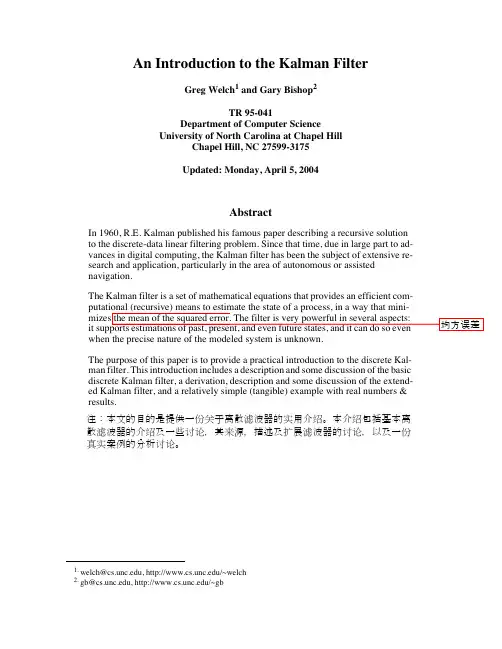
毕业设计(论文)外文资料翻译系 ： 电气工程学院专 业： 电子信息科学与技术 姓 名： 周景龙 学 号： 0601030115 外文出处： Department of Computer Science University ofNorth Carolina at Chapel HillChapel Hill,NC27599-3175附 件：1.外文资料翻译译文；2.外文原文。

(用外文写)卡尔曼滤波器介绍摘要在1960年，卡尔曼出版了他最著名的论文，描述了一个对离散数据线性滤波问题的递归解决方法。

从那以后，由于数字计算的进步，卡尔曼滤波器已经成为广泛研究和应用的主题，特别在自动化或协助导航领域。

卡尔曼滤波器是一系列方程式，提供了有效的计算（递归）方法去估计过程的状态，是一种以平方误差的均值达到最小的方式。

滤波器在很多方面都很强大：它支持过去，现在，甚至将来状态的估计，而且当系统的确切性质未知时也可以做。

这篇论文的目的是对离散卡尔曼滤波器提供一个实际介绍。

这次介绍包括对基本离散卡尔曼滤波器推导的描述和一些讨论，扩展卡尔曼滤波器的描述和一些讨论和一个相对简单的（切实的）实际例子。

离散卡尔曼滤波器在1960年，卡尔曼出版了他最著名的论文，描述了一个对离散数据线性滤波问题的递归解决方法[Kalman60]。

从那以后，由于数字计算的进步，卡尔曼滤波器已经成为广泛研究和应用的主题，特别在自动化或协助导航领域。

第一章讲述了对卡尔曼滤波器非常“友好的”介绍[Maybeck79]，而一个完整的介绍可以在[Sorenson70]找到，也包含了一些有趣的历史叙事。

更加广泛的参考包括Gelb74；Grewal93；Maybeck79；Lewis86；Brown92；Jacobs93].被估计的过程卡尔曼滤波器卡用于估计离散时间控制过程的状态变量n x ∈ℜ。

这个离散时间过程由以下离散随机差分方程描述：111k k k k x Ax bu w ---=++ （1.1）测量值m z ∈ℜ，k k k z Hx v =+ （1.2） 随机变量k w 和k v 分别表示过程和测量噪声。

卡尔曼滤波器介绍Greg Welch1and Gary Bishop2TR95-041Department of Computer ScienceUniversity of North Carolina at Chapel Hill3Chapel Hill,NC27599-3175翻译：姚旭晨更新日期:2006年7月24日，星期一中文版更新日期：2007年1月8日，星期一摘要1960年，卡尔曼发表了他著名的用递归方法解决离散数据线性滤波问题的论文。

从那以后，得益于数字计算技术的进步，卡尔曼滤波器已成为推广研究和应用的主题，尤其是在自主或协助导航领域。

卡尔曼滤波器由一系列递归数学公式描述。

它们提供了一种高效可计算的方法来估计过程的状态，并使估计均方误差最小。

卡尔曼滤波器应用广泛且功能强大：它可以估计信号的过去和当前状态，甚至能估计将来的状态，即使并不知道模型的确切性质。

这篇文章介绍了离散卡尔曼理论和实用方法，包括卡尔曼滤波器及其衍生：扩展卡尔曼滤波器的描述和讨论，并给出了一个相对简单的带图实例。

1welch@,/˜welch2gb@,/˜gb3北卡罗来纳大学教堂山分校，译者注。

1Welch&Bishop,卡尔曼滤波器介绍21离散卡尔曼滤波器1960年，卡尔曼发表了他著名的用递归方法解决离散数据线性滤波问题的论文[Kalman60]。

从那以后，得益于数字计算技术的进步，卡尔曼滤波器已成为推广研究和应用的主题，尤其是在自主或协助导航领域。

[Maybeck79]的第一章给出了一个非常“友好”的介绍，更全面的讨论可以参考[Sorenson70]，后者还包含了一些非常有趣的历史故事。

更广泛的参考包括[Gelb74,Grewal93,Maybeck79,Lewis86,Brown92,Jacobs93]。

被估计的过程信号卡尔曼滤波器用于估计离散时间过程的状态变量x∈ n。

这个离散时间过程由以下离散随机差分方程描述：x k=Ax k−1+Bu k−1+w k−1,(1.1)定义观测变量z∈ m，得到量测方程：z k=Hx k+v k.(1.2)随机信号w k和v k分别表示过程激励噪声1和观测噪声。

卡尔曼滤波是一种高效率的递归滤波器(自回归滤波器), 它能够从一系列的不完全包含噪声的测量(英文:measurement)中，估计动态系统的状态。

应用实例卡尔曼滤波的一个典型实例是从一组有限的，对物体位置的，包含噪声的观察序列预测出物体的坐标位置及速度. 在很多工程应用(雷达, 计算机视觉)中都可以找到它的身影. 同时，卡尔曼滤波也是控制理论以及控制系统工程中的一个重要话题.比如,在雷达中,人们感兴趣的是跟踪目标,但目标的位置,速度,加速度的测量值往往在任何时候都有噪声.卡尔曼滤波利用目标的动态信息,设法去掉噪声的影响,得到一个关于目标位置的好的估计。

这个估计可以是对当前目标位置的估计(滤波),也可以是对于将来位置的估计(预测)，也可以是对过去位置的估计(插值或平滑).命名这种滤波方法以它的发明者鲁道夫.E.卡尔曼（Rudolf E. Kalman）命名. 虽然Peter Swerling实际上更早提出了一种类似的算法.斯坦利.施密特(Stanley Schmidt)首次实现了卡尔曼滤波器.卡尔曼在NASA埃姆斯研究中心访问时,发现他的方法对于解决阿波罗计划的轨道预测很有用,后来阿波罗飞船的导航电脑使用了这种滤波器. 关于这种滤波器的论文由Swerling (1958), Kalman(1960)与 Kalman and Bucy (1961)发表.目前,卡尔曼滤波已经有很多不同的实现.卡尔曼最初提出的形式现在一般称为简单卡尔曼滤波器.除此以外,还有施密特扩展滤波器,信息滤波器以及很多Bierman, Thornton 开发的平方根滤波器的变种.也行最常见的卡尔曼滤波器是锁相环，它在收音机,计算机和几乎任何视频或通讯设备中广泛存在.卡尔曼滤波器– Kalman Filter1．什么是卡尔曼滤波器（What is the Kalman Filter ）在学习卡尔曼滤波器之前，首先看看为什么叫“卡尔曼”。