安捷伦 3000T X 系列示波器说明书
- 格式:pdf
- 大小:6.12 MB
- 文档页数:36
Keysight InfiniiVision 3000T X 系列示波器用户指南声明© Keysight Technologies, Inc. 2005-2022根据美国和国际版权法,未经 Keysight Technologies, Inc. 事先同 意和书面允许,不得以任何形式或通过 任何方式(包括电子存储和检索或翻译 为其他国家或地区的语言)复制本手册 中的任何内容。
手册部件号75037-97089版本第八 版, 2022 年 6 月仅提供电子格式发布者:Keysight Technologies, Inc.1900 Garden of the Gods Road Colorado Springs, CO 80907 USA修订历史75037-97002, 2014 年 11 月75037-97015, 2015 年 8 月75037-97027, 2016 年 7 月75037-97040, 2017 年 11 月75037-97052, 2019 年 5 月75037-97064, 2020 年 10 月75037-97076, 2021 年 10 月75037-97089, 2022 年 6 月担保本文档中包含的材料" 按现状"提供,在将来版本中如有更改,恕不另行通知。
此外,在适用法律允 许的最大范围内,Keysight 不对本手册及其包含的任何信息提供任何明示或暗示的保证,包括但不仅限于对适销性和用于特定用途时的适用性的暗示担保。
对于因提供、使用或运用本文档或其包含的任何信息所导致的错误或者意外或必然损害,Keysight 概不负责。
如果Keysight 和用户之间已达成的单独书面协议包含涉及本文档内容的担保条款,但担保条款与这些条款有冲突,则应以单独协议中的担保条款为准。
技术许可对于本文档中描述的硬件和/或软件,仅在得到许可的情况下才会提供,并且只能根据许可进行使用或复制。
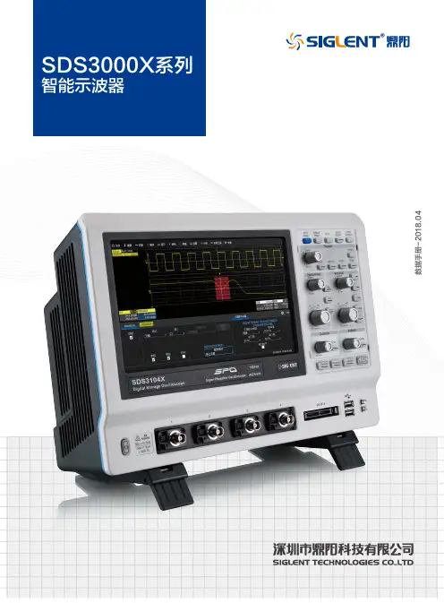
数据手册-2018.04SDS3000X 系列智能示波器数据手册产品综述SDS3000X 系列智能示波器,最大带宽 1GHz,最高实时采样率 4GSa/s,采用创新的 SPO 技术,支持高刷新、256级波形辉度等级及色温显示、数字触发和深存储特性;采用单芯片 ADC,具备优异的模拟前端和信号保真度;支持丰富的智能触发、串行协议触发和解码;支持历史模式(History)、顺序模式(Sequence)、高级波形搜索和分析(WaveScan)、趋势图(Trend)、参数直方图(Histicons)、增强分辨率模式(Eres);具备丰富的测量和数学运算功能;具备独特的综合归档功能(LabNoteBook);支持16路数字通道;集成 25MHz 函数 / 任意波形发生器;配备 Windows 操作系统和10.1 英寸电容触摸屏。
基于以上强大的功能与特性,SDS3000X 可以满足用户日益增长的测试测量和数据分析的需求,是一款性能先进的智能示波器。
特性与优点模拟通道带宽:500MHz、1GHz 4 模拟通道 +1 个外触发通道实时采样率高达 4GSa/s 创新的 SPO 技术 存储深度达 20Mpts/CH 波形捕获率达 1,000,000 帧 / 秒具备优异的模拟前端和信号保真度,最低底噪低于 400μV 支持 256 级波形辉度等级及色温显示配备 Windows 操作系统和 10.1 英寸电容触摸屏(1024*600),支持触摸屏、键盘、 鼠标操作采用顶级的用户界面MAUI,迷人的简洁,所有菜单层级只有两级 集成了 15 种最常用的一键式设计,一触即发智能触发(边沿,脉宽,判定合格,逻辑图,TV,窗口,间隔,漏失,欠幅, 斜率)串行总线触发及解码,支持的协议:I 2C、I 2S、 SPI、 UART/RS232、LIN、CAN、 CAN-FD、 FlexRay、MIL 1553、USB 2.0顺序模式(Sequence),根据用户设置的触发条件,以最小 1us 的死区时 间分段捕获符合条件的事件,并给出时间标签高级波形搜索和分析(WaveScan)功能,支持多种搜索条件,并把捕获的 异常信号用 Zoom 功能展现出来,方便用户在海量信息中快速搜索出需要关 注的波形增强分辨率模式(Eres),通过数字滤波的方式降低噪声带宽,可等效提高 示波器的垂直分辨率,最高可达 11 bit历史模式(History),一键进入,通过导航栏“回放”历史上出现过的波形综合报告归档功能(LabNoteBook), 保存的数据可在示波器和 PC 端进行 再测量和分析24 种参数统计测量和 20 种波形运算,能支持 AIM 测量和波形的运算再运 算(Math on Math)趋势图(Trend),以线图的方式表示参数测量结果随采集的次序变化的过程, 第一次采集的测量结果显示在屏幕的最左边,测量结果从右往左逐渐移动参数直方图(Histicons),反映了参数值在一个确定范围 (Bin) 内出现的概率, 表明了参数值的统计分布状态通过 / 失败(Pass/Fail)检测功能,用户可自定义规则 / 模板,与被测信号 进行比较,实时统计通过 / 失败的次数,可用来查找异常波形或进行自动化测试内置 25MHz 函数 / 任意波形发生器,125MSa/s 采样率,16kpts 波形长度 16 路数字通道(MSO 功能),500MSa/s 采样率,10Mpts 存储深度4 位数字电压表和 5 位硬件频率计功能丰富的外围接口:4*USB Host,SD 卡槽,USB Device,LAN,AUX out (Pass/Fail,Trigger Out),EXT TRIG,标准 D 型 15 针 SVGA 接口(分辨 率 1024*600),16 路逻辑通道接口和可配置的校准信号接口,方便仪器扩 展及程控操作SDS3000X 系列智能示波器数据手册型号与主要指标一键进入运算一键保存一键打印一键清除一键进入历史模式一键调用保存的波形一键复位一键捕获一键放大一键光标一键WaveScan 一键触发点归零同类型500MHzSDS3054XSDS3000X 系列智能示波器数据手册创新的SPO 构架丰富的调试工具包,精确定位问题在实时采样下,SDS3000X 系列最大支持250,000帧/秒的波形捕获率;在顺序模式(Sequence)下,其最高波形捕获率可达1,000,000帧/秒。
安捷伦示波器说明书解决multisim仿真速度慢multisim11.0中仿真时间步长的设定方法multisim10示波器的使用方法——同电子仿真软件MultiSIM 9中的虚拟示波器使用方法2011-06-13 22:16:43| 分类:IC -- 电子| 标签:|字号大中小订阅电子仿真软件MultiSIM 9中的虚拟示波器使用方法朱晓欣(原载《无线电》杂志07年第五期)在电子仿真软件MultiSIM 9中,除了虚拟双踪示波器和虚拟四踪示波器以外,还有两台高性能的先进示波器,它们分别是:跨国"安捷伦"公司的虚拟示波器"Agilent54622D"和美国"泰克"公司的虚拟数字存贮示波器"TektronixTDS2024"。
本刊06年第五期曾对Multisim7中的安捷伦虚拟示波器设置和显示有过简单介绍,读者可以参阅该文相关内容。
本文主要介绍安捷伦虚拟示波器的一些特殊其它功能和美国"泰克"公司的虚拟数字存贮示波器这两台高档次的示波器使用方法。
一、安捷伦虚拟示波器"Agilent54622D"的使用方法举例Agilent54622D虚拟示波器的带宽为100MHz,具有两个模拟通道和16个逻辑通道。
图一是它的放大面板图,它的各个开关、按钮及旋钮的排列和调节都和实物仪器完全一样,我们在自己的电脑里也能享受到使用高档次测量仪器的愉悦,且没有损坏仪器的担忧。
图一一、显示基本波形操作(这里以模拟通道1为例说明)首先在电子仿真软件MultiSIM 9电子平台上调出安捷伦虚拟函数信号发生器和安捷伦虚拟示波器各一台。
并按图二连好电路;双击安捷伦虚拟函数信号发生器图标"XFG1"打开电源开关,不作任何设置使用它的默认值,即:频率1kHz,幅值100mVpp的正弦波(可参阅上期介绍)。
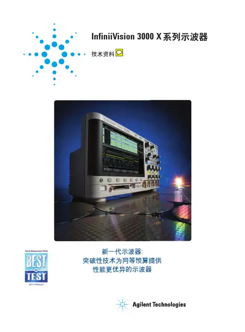
AgilentInfiniiVision 3000X 系列示波器使用者指南s1聲明© Agilent Technologies, Inc. 2005-2012本手冊受美國與國際著作權法之規範,未經 Agilent Technologies, Inc. 事先協議或書面同意,不得使用任何形式或方法 (包含電子形式儲存、擷取或轉譯為外國語言) 複製本手冊任何部份。
手冊零件編號75019-97054版本第五 版, 2012 年 3 月馬來西亞印製Agilent Technologies, Inc.1900 Garden of the Gods Road Colorado Springs, CO 80907 USA 保固本文件所含內容係以「原狀」提供,未來版本若有變更,恕不另行通知。
此外,在相關法律所允許之最大範圍內,Agilent 不承擔任何瑕疵責任擔保與條件,不論其為明示或暗示者,其中包括 (但不限於) 適售性、適合某特定用途以及不侵害他人權益之暗示擔保責任。
對於因提供、使用或運用本文件或其中所含的任何內容,以及所衍生之任何損害或所失利益或錯誤,Agilent 皆不負擔責任。
若Agilent 與使用者就本文件所含材料保固條款簽訂其他書面協議,其中出現與上述條款相牴觸之部分,以個別合約條款為準。
技術授權此文件中所述的硬體及/或軟體係依授權提供,且僅可以依據此類授權之條款予以使用或複製。
限制權利聲明美國政府限制權利。
授予聯邦政府之軟體及技術資料僅包含為一般使用者提供的自訂權利。
Agilent 依照 FAR12.211(「技術資料」) 及 12.212 (「電腦軟體」)、國防部 DFARS 252.227-7015 (「技術資料 - 商業條款」) 以及 DFARS227.7202-3 (「商業電腦軟體」或「電腦軟體說明文件」中的權利) 提供此軟體與技術資料之自訂商業授權:安全聲明「注意」標示代表發生危險狀況。
Agilent DSOX3000 FE演示指南基本介绍和设置目的和说明这个演示指南主要为分销工程师设计,目标是能独立的为客户做10-20分钟演示,把DSOX3000的一些独特的特点、优势和好处介绍给客户。
需要的设备DSOX3000示波器,两根无源探头N28XXA/B.任务一:示波器基本介绍介绍3000X的一些基本概况.包括:1.5合1设备,即是一台综合示波器,逻辑分析仪,协议分析仪,任意波形发生器,电压表和频率计为一体的综合性设备.根据客户应用情况,针对5合1中的子设备功能做重点介绍。
要点:示波器主要型号,带宽,主要采样率指标,带宽可升级,波形捕获率,强大的触发功能等;MSO的基本指标,采样率,存储深度;协议分析仪支持的串行总线种类,硬件协议触发和解码;任意波形发生器,支持的信号类型和最高频率;电压表和频率计的基本指标。
2.对产品的简洁外形做一简单介绍.3. 针对每个子设备功能能熟练的做自动演示。
任务二:100万次/秒的波形捕获率,信号捕获和触发介绍简介中低端示波器日常主要应用为通用信号调试和观察,因此如何演示3000X的调试和捕获功能无疑是非常重要的.此任务演示主要和TEK DPO3000/4000演示对应,需要展示出3000X在调试能力方面全面超越DPO3000/4000的特点.首先请按自动演示介绍DSOX3000 100万次/秒波形捕获率及与其它竞争对手产品指标差异及对比效果。
其次,采用内部信号做模拟实测演示。
设置步骤:1.连接通道1到Demo1端子和地,通道2到Demo2端子和地。
2.按下Default Setup.按下Help,然后按下培训信号软键,旋转多功能旋钮选择带偶发毛刺的时钟信号,按下右下角输出按钮。
可以看到如下波形:3.调节垂直和水平档位及触发到500mV/Div,20ns/Div,边沿触发在1V/Div,得到如下波形:这时可以看到偶发毛刺信号在闪烁,并强调DSOX3000 业界领先的100万次/秒的波形捕获率可以最快看到这一偶发信号。
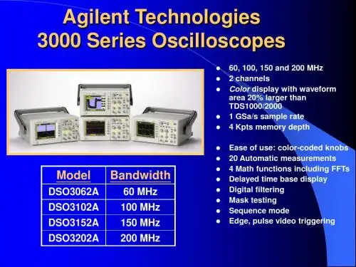
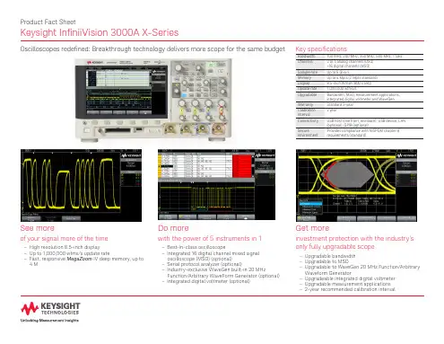
Agilent Technologies 3000 Series Oscilloscopes Data SheetGet more for your moneyAgilent’s 3000 Series oscilloscopes give you an affordable way tosee what’s happening in your designs. Developed with the features you need to make your job easier – including a large LCD color display. Need flexibility? Choose from four models with bandwidths ranging from 60-MHz to 200-MHz. To give you the debugging power you need, each oscilloscope comes standard with advanced features including sophisticated triggering, automatic measurements,digital filtering, sequence mode acquisition,math functions (including FFTs), stored setups and waveforms, mask testing and much more.Full-featured oscilloscopes for the smallest budgetsFeatures:• 60 to 200 MHz bandwidths• 1 GSa/s maximum sample rate• Large 15-cm (5.7-in) color display• Advanced triggering includingedge, pulse width, and line-selectable video• 4 kpts of waveform memory• USB host and device connectivity,standard• 20 automatic measurements plushardware counter and Measure All• Four math functions, includingFFTs standard• Mask test standard• GPIB and RS-232 connectivity andSCPI programming available withN2861A communications module• Interface localized into12-languages• Sequence mode (segmentedmemory) standardSee your signals more clearlyAll 3000 Series models have color Array displays to allow you to quicklyidentify your signals, and thelarge size – 15-cm (5.7-in) with320 x 240 resolution – makesit easier for you to see moreinformation.The 3000 Series’ delayed sweepalso lets you see more details inyour design. You can view a longrecord, then window in on thesection of the signal of interest.Figure 1. All 3000 Series oscilloscopes come standard witha color display and cost 20% less than competitive products.The color display allows you to quickly and easily identify yoursignals and view signal activity. ArrayFigure 2. Want to see the big picture but still get all thedetails? Use the delayed sweep mode to zoom in on aparticular area of interest on your signal while still viewingthe entire captured waveform.2The features you needAll 3000 Series scopes include the standard features you need to get your job done easier and faster: Autoscale – Autoscale lets you quickly display any active signals, automatically setting the vertical, horizontal and trigger controls for the best signal display.Easy connectivity – The 3000 Series oscilloscopes come standard with an N2865A USB host module for saving setups, waveforms and displays to a memory stick. This port is also compatible with many USB printers.This scope series also offers Scope Connect software, which provides PC connectivity for data gathering, pass/fail testing, and analysis via the 3000 Series' USB device port.GPIB and RS-232 interfaces are also available with the N2861A connectivity module.Advanced triggering –Includes edge, pulse width and line-selectable video, to help you isolate the signals you want to see.20 automatic measurements – To save time, you can make18 different measurements simultaneously.Figure 3. The 3000 Series comes equipped with a broad set of measurement and math features, including FFTs at no additional cost. You can choose between 4 FFT windows for your specific measurement needs: Hanning, Hamming,Blackman-Harris, and rectangular.Waveform math with FFTs– Analysis functions includeaddition, subtraction,multiplication, and Fast FourierTransforms with four windows(Hanning, Hamming, Blackman-Harris and rectangular).Auto calibration – Automaticallycalibrates the oscilloscope’svertical and horizontal systems.Multi-language interface –Operate the oscilloscope inthe language of your choice.Language support includessimplified and traditionalChinese, Japanese, Korean,French, German, Italian,Portuguese, Russian, Spanishand English.Figure 4. Standard USB host and device ports allow you to send your measurements directly to your PC or save them to Flash memory sticks.34The features you need (continued)Digital filtering – Digital filtering selections include low pass, high pass, band pass, and band reject filters. Limits are selectablebetween 1-kHz and the bandwidth of your oscilloscope model.Ten waveform and setupmemories – Store waveforms or commonly used setups for future reference and use.Mask testing – Automatically compares incoming signals with a pre-defined mask, clearly highlighting signal changes.Sequence mode (segmented memory) – Frame an area of interest on your signal for acquisition and record up to 1,000 frames for playback.Pulse triggering – Lets you trigger on pulse events.3-year warranty – All 3000Series scopes include a full 3-year warranty.Easy to set up and use– Dedicated, color-coded knobs for vertical sensitivity, offset, and time base settings make it easy to set up and use. Front-panel keys for triggering functions are alsogrouped to make your job easier.Figure 7. With dedicated, color-coded knobs and front-panel keys grouped by function, it is easy to find and use all of the features of the scope – from the most basic to the more advanced functions.Figure 5. The digital filter capability enhances your ability to examine important signal components by filtering out undesired spectral components such as various typesof noise.Figure 6. Use the sequence mode to frame an area of interest on your signal for acquisition; then, use the playback feature to quickly play through the sequence andeasily spot glitches or other signalanomalies.Performance characteristics567Ordering information89Ordering information(continued)To get a Quick Quote on Agilent3000 Series oscilloscopes, go to /find/dso3000Call the measurement experts at Agilent TechnologiesWhether your work is mostly digital, mostly analog, orsomewhere in the middle, our measurement specialists can help you select the best debugging solution. Call today to talk to a knowledgeable engineer about your particular application.10Agilent Technologies OscilloscopesMultiple form factors from 20 MHz to >90 GHz | Industry leading specs | Powerful applications。
DSOX3PWR 功率量測應用使用者指南s1聲明© Agilent Technologies, Inc. 2007-2009, 2011-2012本手冊受美國與國際著作權法之規範,未經 Agilent Technologies, Inc. 事先協議或書面同意,不得使用任何形式或方法 (包含電子形式儲存、擷取或轉譯為外國語言) 複製本手冊任何部份。
手冊零件編號版本 02.20.0000版本2012 年 7 月 16 日Available in electronic format onlyAgilent Technologies, Inc.1900 Garden of the Gods Road Colorado Springs, CO 80907 USA 保固本文件所含內容係以「原狀」提供,未來版本若有變更,恕不另行通知。
此外,在相關法律所允許之最大範圍內,Agilent 不承擔任何瑕疵責任擔保與條件,不論其為明示或暗示者,其中包括 (但不限於) 適售性、適合某特定用途以及不侵害他人權益之暗示擔保責任。
對於因提供、使用或運用本文件或其中所含的任何內容,以及所衍生之任何損害或所失利益或錯誤,Agilent 皆不負擔責任。
若Agilent 與使用者就本文件所含材料保固條款簽訂其他書面協議,其中出現與上述條款相牴觸之部分,以個別合約條款為準。
技術授權此文件中所述的硬體及/或軟體係依授權提供,且僅可以依據此類授權之條款予以使用或複製。
限制權利聲明美國政府限制權利。
授予聯邦政府之軟體及技術資料僅包含為一般使用者提供的自訂權利。
Agilent 依照 FAR12.211(「技術資料」) 及 12.212 (「電腦軟體」)、國防部 DFARS 252.227-7015 (「技術資料 - 商業條款」) 以及 DFARS227.7202-3 (「商業電腦軟體」或「電腦軟體說明文件」中的權利) 提供此軟體與技術資料之自訂商業授權:安全聲明注意「注意」標示代表發生危險狀況。
安捷伦⽰波器使⽤⽅法Jitter Analysis Techniques Using an Agilent Infiniium OscilloscopeProduct NoteIntroductionWith higher-speed clocking and data transmission schemes in the computer and communications industries, timing margins are becoming increasingly tight.Sophisticated techniques are required to ensure that timing margins are being met and to find the source of problems if they are not.This product note discussesvarious techniques for measuring jitter and points out theiradvantages and disadvantages. It describes how to set up an Agilent Infiniium oscilloscope to make effective jitter measure-ments and the accuracy of these measurements. Some of themeasurement techniques are only available on Agilent 54845A/B and 54846A/B oscilloscopes with version A.04.00 or later software.These measurement techniques are indicated as such in the text.Jitter FundamentalsJitter is defined as the deviation of a transition from its ideal time.Jitter can be measured relative to an ideal time or to another transition. Several factors can affect jitter. Since jitter sources are independent of each other,a system will rarely encounter a worst-case jitter scenario. Only when each independent jitter source is at its worst and is aligned with the other sources will this occur. As a result, jitter is statistical in nature. Predicting the worst-case jitter in a system can take time.Jitter can be broken down into two categories:Random jitter is uncorrelated jitter caused by thermal or other physical, randomprocesses. The shape of the jitter distribution is Gaussian.For example, a well-behaved phase lock loop (PLL) wanders randomly around its nominal clock frequency.?Deterministic or systematic jitter can be caused by inter-symbol interference,crosstalk, sub-harmonicdistortion and other spurious events such as power-supply switching. It is important to understand the nature of the jitter to help diagnose its cause and, if possible, correct it. Deterministic jitter is more easily reduced or eliminated once the source has been identified.Jitter Measurement TechniquesThis product note will discuss four methods that can be used to characterize jitter in a system:Infinite persistenceHistogramsMeasurement statisticsMeasurement functionsInfinite PersistenceAgilent’s Infiniium oscilloscopes present several different views of jitter. One way to measure jitter is to trigger on one waveform edge and look at another edge while infinite persistence is turned on. To use this technique, set up the scope to trigger on a rising or falling edge and set the horizontal scale to examine the next rising or falling edge. In the Display dialog box, set persistence to infinite.This technique measurespeak-to-peak jitter and does not provide information about jitter distribution. Infinite persistence is easy to set up and will acquire data quickly, giving you the best chance to see worst-case jitter. However, since the tails of the jitter distribution theoretically go on forever, it will take a long time to measure the worst-case, peak-to-peak jitter.It is important to understandtheerror sources of this measurement. This technique is subject to oscilloscope trigger jitter–the largest contributor to timingerror in an oscilloscope. Trigger jitter results from the failure to place the waveform correctly relative to when a trigger event occurs. Since the infinite persistence technique overlaps multiple waveform acquisitions onto the scope display, and each acquisition is subject to trigger jitter, the accuracy of this technique can be limited. If your jitter margins are being met using this technique, then more advanced measurement techniques are not necessary. This product note will discuss Infiniium’s timebase and trigger specifications in detail in alater section.HistogramsThis technique not only shows worst-case jitter, but also gives a perspective on jitter distribution. Histograms do not acquire infor-mation as quickly as infinite persistence since each acquisition must be counted in the histogram measurement.To set up a histogram, trigger on an edge and set the horizontalscale and position so that you canview the next rising or fallingedge. In the Histogram dialog box,turn on a horizontal histogramand set both Y window markersto the same voltage. For example,if a clock threshold is at 800 mV,set both Y markers to this voltage.Set the X markers to the left andright of the edge (figure 1). Figure 1. Histogram of edge showing bi-modal distribution23It is often possible to determine if the jitter is random or deter-ministic by the shape of the histogram. Random jitter will have a Gaussian distribution.Infiniium displays the percentage of points within mean +/- 1, 2,and 3 standard deviations to help in determining how Gaussian the distribution is. For a Gaussian distribution these values should be 68%, 95%, and 99.7%, respec-tively. Non-Gaussian distributions usually indicate that the jitter has deterministic components.This technique has the same limitation on accuracy as the infinite persistence technique.Multiple acquisitions contribute to the histogram and they all contain the oscilloscope trigger jitter mentioned above. Measurement StatisticsThe next method involvescomputing statistics on waveform measurement results. For example,the scope can measure the period of a waveform on successive acquisitions. Simply drag the period measurement icon to the waveform that is to be measured.The statistics will indicate the mean, standard deviation, and min and max of the period measurements. You can let the scope run for a while to determine the amount of clock jitter present. This measurement is not subject to trigger jitter because it is a delta-time or relative measure-ment. Even if the waveform is not placed correctly relative to the trigger, the edges are measuredaccurately relative to each other.Figure 2. Setting up a jitter measurementThis measurement is subject to the timebase stability of the instrument, which is typically very good. This is a valid measurement technique but is slow to gather statistical information. Since the scope acquires a waveform, makes a measurement, and then acquires a waveform at a later time, most clock periods are not measured.With this technique, it is impossible to see how the period jitter varies over short periods of time. For example, if you have spread-spectrum clocking, this measurement will lump the slowest and fastest periods together.The Agilent 54845A/B and54846A/B Infiniium oscilloscopes can compute statistics on every instance of a measurement in asingle acquisition. To enable this capability, select the Jitter tab,then check “Measure all edges” in the Measurement Definitions dia-log box (figure 2).For example, instead of only measuring the first period on every acquisition or trigger event,every period can be measured and statistics gathered. This greatly increases the speed at which statistics are gathered and reduces the overall time to make jitter measurements. Statistics are accumulated across allmeasurements in the acquisition and across acquisitions.Pressing “Clear Display” will reset the measurement statistics.This feature is useful if you are probing the clock at different locations and want to reset the measurements.It is important to set up the scope correctly to make effective jitter measurements. Set the vertical scale of the channel being measured to offer the largest waveform that will fit on screen vertically. This will make the most effective use of the scope’s A/D converter.The scope should be set toreal-time acquisition mode inthe Acquisition dialog box. Since equivalent-time sampling can combine samples from different acquisitions, the scope’s trigger jitter would adversely affect jitter measurements. The averaging function should be turned off since, again, this combines multiple acquisition data.You may want to set the scopeto its maximum memory depth. This will make the scope less responsive to operate, but the scope can make many measure-ments on a single acquisition. Since jitter measurements are statistical, many measurements are desirable. Taking many acquisitions of small records will give a more random selection but will take longer than fewer large acquisitions. Having extremely deep memory is not necessary to getting good jitter measurements. Normally, measurements aremade at 10%, 50%, and 90% of thewaveform amplitude. This isconvenient for quickly makingmeasurements; however, whenmaking measurements acrossacquisitions and combiningtheir statistics this is not thebest solution.In the Measurement Definitiondialog box, Thresholds tab, themeasurement thresholds shouldbe set to absolute voltages. Forexample, if you are makingcycle-cycle jitter or periodmeasurements, set the middlevoltage threshold to your clockthreshold. Set the upper andlower voltage thresholds toroughly +/- 10% of the signalamplitude in voltage. This willestablish a band around thethreshold that the edge must gothrough to be measured and willeliminate false edge detection.In addition to the period jitter measurement, the cycle-cycle jitter measurement uses the same technique. The cycle-cycle jitter measurement, available on Agilent 54845A/B and 54846A/B oscilloscopes, is the differenceof two consecutive period measurements.Pi – P(i-1), 2 ≤i ≤nWhereP is a period measurement and n is the number of periods inthe waveform.Cycle-cycle jitter is a measure of the short-term stability of a clock. It may be acceptable for the clock frequency to change slowly over time but not vary from cycle to cycle. For this measurement, every period in the acquisition is measured regardless of how the “Measure all edges” selection is set. In this case, the statistics represent all of the cycle-cycle jitter measurements in one acquisition, or all acquisitionsif the scope is running.If absolute clock stability is required, then a period measurement should be made. If your system can track with small changes in the clock frequency, then cycle-cycle jitter should be measured.Again, if your timing marginsare being met with thistechnique, more advancedtechniques are not necessary. Itis only fairly recently that tightertiming margins have causedengineers to need other jittermeasurement techniques.45Measurement FunctionAgilent 54845A/B and 54846A/B Infiniium oscilloscopes can plot measurement results correlated to the signal being measured. For example, if every period is meas-ured, as in the case above, the measurement function will plot period measurement results on the vertical axis, time-correlated to the waveform that the period measurement is measuring (figure 3).In this example, the secondperiod is slightly longer than the first. The third period is shorter than the second. Also notice that the lengths of the measurement function lines correspond to the period and their placement corresponds to channel 1 because we are measuring period on channel 1.Using this technique, the shape of the jitter is apparent. For example, with spread-spectrum clocking you can see the modulation frequency as the period gets progressively slower and faster. This allows you to see sinusoidal shapes or other patterns in the measurement function plot (figure 4). It is also possible to correlate poor jitter results with the source waveform that caused them. This can aid not only in your design but can also ensure that the scope is measuring appropriate voltage levels when gatheringjitter statistics.Figure 3. Measurement function on a few cyclesFigure 4. Measurement function on many cyclesTo turn on the measurement function, first turn on the desired measurement to track. Measurements that can be tracked with the measurement function are rise time, fall time, period, frequency, cycle-cycle jitter, + width, - width and duty cycle. The measurement function is enabled in the Waveform Math dialog box (figure 5). Select a function that is a different color than the channel you are measuring to make it easier to see. Set the function operator to “measurement.” Select the measurement you wish to track and turn on the measurement function. The math function now plots the measurement results on the vertical axis, time-correlated to the channel being measured. Only one measurement function can be enabled at a time; however, the function can beset to track any of the currently active measurements listed above.Set up the acquisition by selectingthe maximum memory depth inthe Acquisition dialog box. Turnoff averaging and Sin(X)/Xinterpolation in the Acquisitiondialog box. Set the sample rateso that you are getting at leastseveral sample points on theedges that you are measuring.Measurements are made on thedata that is windowed by thescreen. To see something slowerthat may be coupling into yourclock, for example, you will needto compress the channel data onthe screen.Now that the memory depth andsample rate are fixed, you canadjust the horizontal scale sothat all of the acquired data ison screen. In order to make fulluse of the A/D converter andseparate the waveforms on thedisplay, you may want to split thegrid into two parts. If you havea very dense waveform that isbeing measured, it will be nearlyimpossible to see the measurementfunction on top of it. Turn on thesplit grid in the Display dialog box. Figure 5. Setting up a measurement function6Sources of Measurement ErrorIn this section we will examine some of the principal sources of jitter measurement error. For best accuracy, the scope should be making measurements at the same temperature as when the scope was last calibrated. If the temperature has varied by more than 5 degrees, the softwareself-calibration should be performed again. The Calibration dialog box shows the change from the calibration temperature. Trigger JitterThe most common source of error across multiple acquisitions is trigger jitter. This is the error associated with placing the first point and all subsequent points of the waveform relative towhen the trigger occurs.For Infiniium models 54830B, 54831B, and 54832B, trigger jitter is 8 ps RMS. For the 54845A/B and 54846A/B, trigger jitter is8ps RMS. Figure 6 shows a 54845B measuring its trigger jitter using its own aux out signal. If the jitter is Gaussian, youcan convert RMS jitter topeak-to-peak jitter by multiplyingthe RMS jitter by 6. Trigger jitteris only relevant if you aremeasuring absolute times asopposed to relative times. Forexample, the histogram techniquedescribed above has this errorsource, but a period measurementdoes not since it is a delta-time orrelative measurement.Figure 6. Histogram of trigger jitterThis source of error can also bepresent in period measurementsif the scope is in equivalent time.In equivalent time, the scope maycombine data points from multipleacquisitions. The scope alsocombines points from multipleacquisitions in real-time averagingmode. If it is possible, jittermeasurements should be maderelative to other edges inreal-time, non-averaged mode.78Sources of Measurement Error (continued)Timebase StabilityInfiniium uses a highly stable crystal oscillator as a source for the sample clock. Errors resulting from instability of the timebase are the least significant. Timebase stability is not a specified quantity but is typically 5 ps RMS for the 54845 and 54846. For the 54830,54831, and 54832, it is typically 2ps RMS. These measurements were made at the sametemperature as the calibration.Vertical NoiseErrors in the vertical portion of the signal path including the A/D converter and preamplifier also contribute to the scope’s jitter.Any misplacement of thewaveform vertically will translate through the slew rate of the signal into time error (figure 7). If the slew rate of the signal atthe point of measurement issteep, then the vertical error will translate into a small time jitter.If the slew rate is slow, however,this can be the most significantsource of error.Figure 7. How vertical errors contribute to time errorsAliasing and InterpolationFrom the previous section, it is clear that the signal should have a high slew rate to alleviate vertical errors. However, this can lead to signal aliasing. If the signal is not sampled sufficiently, significant time errors will be present up to the sample interval. When the scope makes measurements, it interpolates the samples above and below the measurement threshold to get the time of the level crossing. If the interpolation filter is enabled, up to 16interpolated points may be placed between two adjacent acquisition samples. Beyond this, linearinterpolation is used to determine the threshold crossing times.However, samples will only be added if the record length is less than 16K samples.A Case StudyTo illustrate how to use the jitter analysis capability of an Agilent Infiniium oscilloscope, let’s examine a typical problem. You suspect that your power supply or another slower speed clock is coupling into the main clock on the board that you are designing. In order to understand how to eliminate the problem, you would like to know the frequency and wave shape of the signal that is coupling into your clock. Traditionally, you would use an FFT magnitude spectrum and look at the side bands from the fundamental. For example, in figure 8 we have acquired a long record of a number of clock pulses and computed the FFT magnitude with a waveform math function. After we zoom in on the fundamental frequency of the clock, you can see side bands.If we take the difference in frequency from the fundamental to the nearest side band, we can determine the frequency of the coupling signal. In this example, it is measured at 198 kHz. We can also notice the odd harmonics and guess that the coupling signal would not be a sine wave. The resolution of the FFT will not give us a great deal of accuracy in determining the frequency, and we can not really see the shape of the coupling signal.To solve this problem using thejitter analysis capability, we needto think about the problem in adifferent way. If a slower signalwere modulating a higherfrequency signal, then we wouldexpect the period of the higherfrequency signal to get slightlylonger, then slightly shorter, etc.,according to the slower signal(figure 8). The measurementfunction method described earlierin this product note could beused to plot how the periodchanges across the waveform.To set up the scope, acquirethe channel data with a longacquisition record in real-timeacquisition mode. Put all of thewaveform on screen by settingthe sample rate to manual andadjusting the time per division.This will allow you to see how theperiod varies across the entireacquisition. In the MeasurementDefinitions dialog box, Jitter tab,set the control to Measure AllEdges (figure 2). Now, turn ona period measurement. In theMath dialog box, turn on theMeasurement function and setto the period measurement. Figure 8. FFT of clock910A Case Study (continued)You can now see how the period measurement varies across the signal (figure 9). Adjust the time per division until you can see several periods of the slower speed signal in the measurement function. To measure the frequency, use the markers or simply drag the frequencymeasurement to the measurement function. Using this technique, we measure 197 kHz and we can see that the signal is a square wave.This confirms that another signal on the board is coupling into the clock. Armed with this knowledge,we are better equipped to find a solution.SummaryThis product note presents several methods for measuring jitter with Agilent’s Infiniium oscilloscopes. The following quick reference will help you choose the best method for a number of circumstances. Infinite PersistenceShows absolute time or edge jitter Works best when the jitter to be measured is greater than the scope’s jitter Sets up easily ?Acquires data quickly ?Measures only worst-case,peak-to-peak jitterFigure 9. Measurement function showing coupling signalHistogramsShows absolute time or edge jitter Works best when the jitter to be measured is greater than the scope’s jitter Shows a distribution of the jitterHelps determine if the jitter is random or deterministic Measures worst-case, peak-to-peak jitter Measures RMS jitterMeasurement StatisticsShows worst-case, peak-to-peak delta time or measurement jitter Sets up easily Measurement FunctionsShows how measurements vary as a function of timeShows the shape and frequency of a jitter source Helps determine if the jitter is random or deterministic/doc/e26170104431b90d6c85c778.htmlAgilent Technologies’ Test and Measurement Support, Services, and AssistanceAgilent Technologies aims to maximize the value you receive, while minimizing your risk and problems. We strive to ensure that you get the test and measurement capabilities you paid for and obtain the support you need. Our extensive support resources and services can help you choose the right Agilent products for your applications and apply them successfully. Every instrument and system we sell has a global warranty. Support is available for at least five years beyond the production life of the product. Two concepts underlie Agilent's overall support policy: "Our Promise" and "Your Advantage."Our PromiseOur Promise means your Agilent test and measurement equipment will meet its advertised performance and functionality. When you are choosing new equipment, we will help you with product information, including realistic performance specifications and practical rec-ommendations from experienced test engineers. When you use Agilent equipment, we can verify that it works properly, help with product operation, and provide basic measurement assistance for the use of specified capabilities, at no extra cost upon request. Many self-help tools are available.Your AdvantageYour Advantage means that Agilent offers a wide range of additional expert test and meas-urement services, which you can purchase according to your unique technical and business needs. Solve problems efficiently and gain a competitive edge by contracting with us for cal-ibration, extra-cost upgrades, out-of-warranty repairs, and on-site education and training, as well as design, system integration, project management, and other professional engineering services. Experienced Agilent engineers and technicians worldwide can help you maximize your productivity, optimize the return on investment of your Agilent instruments and sys-tems, and obtain dependable measurement accuracy for the life of those products./doc/e26170104431b90d6c85c778.html /find/emailupdatesGet the latest information on the productsand applications you select.By internet, phone, or fax, get assistance with all your test & measurement needsOnline assistance:/doc/e26170104431b90d6c85c778.html /find/assistPhone or FaxUnited States:(tel) 800 452 4844Canada:(tel) 877 894 4414(fax) 905 282 6495China:(tel) 800 810 0189(fax) 800 820 2816Europe:(tel) (31 20) 547 2323(fax) (31 20) 547 2390Japan:(tel) (81) 426 56 7832(fax) (81) 426 56 7840Korea:(tel) (82 2) 2004 5004(fax) (82 2) 2004 5115Latin America:(tel) (305) 269 7500(fax) (305) 269 7599Taiwan:(tel) 0800 047 866(fax) 0800 286 331Other Asia Pacific Countries:(tel) (65) 6375 8100(fax) (65) 6836 0252Email: tm_asia@/doc/e26170104431b90d6c85c778.htmlProduct specifications and descriptions in this document subject to change without notice. Agilent Technologies, Inc. 2002 Printed in USA October 15, 20025988-6109EN。