基于MATLAB的贝叶斯网络(BNT)工具箱的使用与实例
- 格式:ppt
- 大小:692.00 KB
- 文档页数:18
机器学习中的贝叶斯网络及其推理分析张慧莹;宁媛;邵晓非【摘要】机器学习作为当今国内外研究的热点在智能系统中得到了重视和运用,贝叶斯是机器学习的核心方法之一,以贝叶斯理论作为中心的贝叶斯网络必将应用延伸到各个问题领域,本文介绍了贝叶斯网络的概念及其学习推理过程,并结合MATLAB中的BNT工具箱,引用来自UCI的标准数据集对贝叶斯网络进行仿真测试.【期刊名称】《现代机械》【年(卷),期】2012(000)002【总页数】4页(P91-94)【关键词】机器学习;贝叶斯网络;MATLAB;贝叶斯学习推理;BNT工具箱【作者】张慧莹;宁媛;邵晓非【作者单位】贵州大学电气工程学院,贵州贵阳550003;贵州大学电气工程学院,贵州贵阳550003;贵州大学电气工程学院,贵州贵阳550003【正文语种】中文【中图分类】TP1830 引言机器学习作为当今国内外研究的热点,在智能系统中得到了重视和运用,而贝叶斯是机器学习的核心方法之一,以贝叶斯理论作为中心的贝叶斯网络更是将应用延伸到各个问题领域,所有需要作出概率预测的地方都可以见到贝叶斯的影子,这背后的深刻原因在于现实世界本身就是不确定的,人类的观察能力是有局限性的,这正是贝叶斯网络的优点,值得深入研究。
1 机器学习机器学习即是研究计算机怎样模拟或实现人类的学习行为,以获取新的知识或技能,重新组织已有的知识结构使之不断改善自身的性能。
对于机器学习的研究成果已经无声的走入了人类的日常生活,自动驾驶、智能机器手、智能窗帘等等很多方面都可以看到机器学习的应用,它不仅为人类的生活带来了便利,也引领着全世界进入一个智能化的多元世纪。
机器学习旨在建立学习的计算理论,构造各种学习系统,并在各个领域应用这些系统,它有四个构成要素:环境、学习环节、知识库和执行环节[1]。
四个环节之间构成了如图1 所示的关系流程,即“认识—实践—再认识”,从而实现机器学习的过程。
这样一个动态的学习过程表明,机器学习实际是一个有特定目的的知识获取过程,对知识的认识是机器学习研究的基础,知识的获取和提高是机器学习的两个重要内容。

Matlab中的机器学习和贝叶斯网络技巧机器学习是一门涵盖统计学、人工智能和计算机科学等多学科知识的领域,它通过让计算机从数据中学习并逐步改进性能,来完成特定任务。
而贝叶斯网络是机器学习中一种常用的概率图模型,它能够建模和推断变量之间的依赖关系。
本文将介绍在Matlab中应用机器学习和贝叶斯网络的技巧和方法。
一、机器学习基础机器学习的基本任务是通过对已有数据的学习来构建一个预测模型,并用该模型对新的数据进行预测。
在Matlab中,我们可以使用一些常用的机器学习工具箱,如Statistics and Machine Learning Toolbox和Neural Network Toolbox等,来实现各种机器学习算法。
1. 数据准备在进行机器学习之前,我们首先需要准备好适合建模的数据。
这包括数据的采集、预处理和特征提取等步骤。
Matlab提供了丰富的数据处理和可视化函数,如readtable、preprocess和feature_extraction等,来帮助我们完成这些任务。
2. 特征选择在建模之前,我们需要从原始数据中选择出对预测结果有重要影响的特征。
Matlab中提供了一些特征选择工具函数,如sequentialfs、relieff和lasso等,可以帮助我们进行特征选择。
3. 模型训练在数据准备和特征选择之后,我们就可以使用机器学习算法进行模型训练了。
根据不同的问题和数据类型,我们可以选择适合的算法,如支持向量机、决策树、随机森林等。
Matlab提供了这些算法的实现函数,如svmtrain、treefit和randomForest等,可以方便地进行模型训练。
4. 模型评估模型训练完成后,我们需要对模型进行评估,以了解其性能和泛化能力。
在Matlab中,我们可以使用一些评估指标,如准确率、精确率、召回率和F1值等,来评估模型的效果。
此外,还可以使用交叉验证、学习曲线和混淆矩阵等方法来进行模型评估。
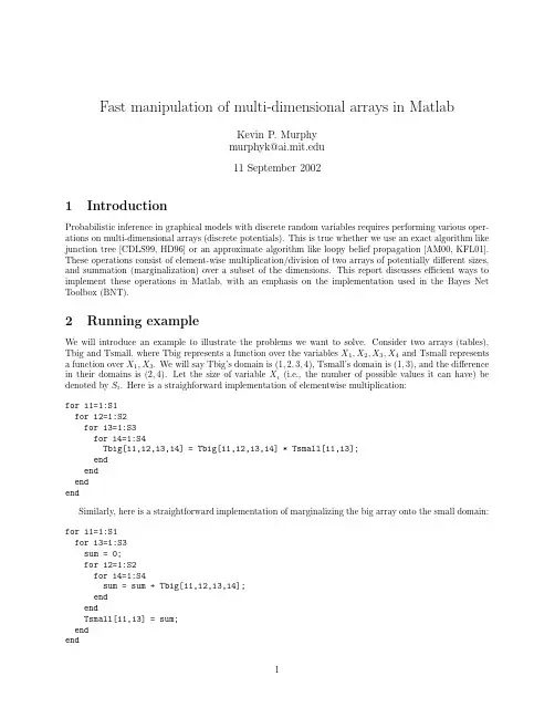
Fast manipulation of multi-dimensional arrays in MatlabKevin P.Murphy**************.edu11September20021IntroductionProbabilistic inference in graphical models with discrete random variables requires performing various oper-ations on multi-dimensional arrays(discrete potentials).This is true whether we use an exact algorithm like junction tree[CDLS99,HD96]or an approximate algorithm like loopy belief propagation[AM00,KFL01]. These operations consist of element-wise multiplication/division of two arrays of potentially different sizes, and summation(marginalization)over a subset of the dimensions.This report discusses efficient ways to implement these operations in Matlab,with an emphasis on the implementation used in the Bayes Net Toolbox(BNT).2Running exampleWe will introduce an example to illustrate the problems we want to solve.Consider two arrays(tables), Tbig and Tsmall,where Tbig represents a function over the variables X1,X2,X3,X4and Tsmall represents a function over X1,X3.We will say Tbig’s domain is(1,2,3,4),Tsmall’s domain is(1,3),and the difference in their domains is(2,4).Let the size of variable X i(i.e.,the number of possible values it can have)be denoted by S i.Here is a straighforward implementation of elementwise multiplication:for i1=1:S1for i2=1:S2for i3=1:S3for i4=1:S4Tbig[i1,i2,i3,i4]=Tbig[i1,i2,i3,i4]*Tsmall[i1,i3];endendendendSimilarly,here is a straightforward implementation of marginalizing the big array onto the small domain: for i1=1:S1for i3=1:S3sum=0;for i2=1:S2for i4=1:S4sum=sum+Tbig[i1,i2,i3,i4];endendTsmall[i1,i3]=sum;endendOf course,these are not general solutions,because we have hard-coded the fact that Tbig is4-dimensional, Tsmall is2-dimensional,and that we are marginalizing over dimensions2and4.The general solution requires mapping vectors of indices(or subscripts)to1dimensional indices(offsets into a1D array),and vice versa. We discuss these auxiliary functions next,before discussing a variety of different solutions based on these functions.3Auxiliary functions3.1Converting from multi-dimensional indices to1D indicesIf a d-dimensional array is stored in memory such that the left-most indices toggle fastest(as in Matlab and Fortran—C follows the opposite convention,toggling the right-most indices fastest),then we can compute the1D index from a vector of indices,subs,as follows:ndx=1+(i1-1)+(i2-1)*S1+(i3-1)*S1*S2+...+(id-1)*S1*S2*...*S(d-1) where the vector of indices is subs=(i1,...,i d),and the size of the dimensions are sz=(S1,...,S d). (We only need to add and subtract1if we use1-based indexing,as in Matlab;in C,we would omit this step.)This can be written more concisely asndx=1+sum((subs-1).*[1cumprod(sz(1:end-1))])If we pass the subscripts separately,we can use the built-in Matlab functionndx=sub2ind(sz,i1,i2,...)BNT offers a similar function,except the subscripts are passed as a vector:ndx=subv2ind(sz,subs)The BNT function is vectorized,i.e.,if each row of subs contains a set of subscripts.then ndx will be a vector of1D indices.This can be computed by simple matrix multiplication.For example,ifsubs=[111;211;...222];and sz=[222],then subv2ind(sz,subs)returns[12...8]’,which can be computed usingcp=[1cumprod(siz(1:end-1))]’;ndx=(subs-1)*cp+1;If all dimensions have size2,this is equivalent to converting a binary number to decimal.3.2Converting from1D indices to multi-dimensional indicesWe convert from1D to multi-D by dividing(which is slower).For instance,if subs=(1,3,2)and sz= (4,3,3),then ndx will bendx=1+(1−1)∗1+(3−1)∗4+(2−1)∗4∗3=21To convert back we geti1=1+ (21−1)mod41=1i2=1+ (21−1)mod124=3i3=1+ (21−1)mod3612=2The matlab and BNT functions sub2ind and subv2ind do this.Note:If all dimensions have size2,this is equivalent to converting a decimal to a binary number.3.3Comparing different domainsIn our example,Tbig’s domain was(X1,X2,X3,X4)and Tsmall’s domain was(X1,X3).The identity of the variables does not matter;what matters is that for each dimension in Tsmall,we canfind the corresponding/ equivalent dimension in Tbig.This is called a mapping,and can be computed in BNT usingmap=find_equiv_posns(small_domain,big_domain)(In R,this function is called match.In Phrog[Phr],this is called an RvMapping.)If smalldom=(1,3) and bigdom=(1,2,3,4),then map=(1,3);if smalldom=(8,2)and bigdom=(2,7,4,8),then map= (4,1);etc.4Naive methodGiven the above auxiliary functions,we can implement multiplication as follows:map=find_equiv_posns(Tsmall.domain,Tbig.domain);for ibig=1:prod(Tbig.sizes)subs_big=ind2subv(Tbig.sizes,ibig);subs_small=subs_big(map);ismall=subv2ind(Tsmall.sizes,subs_small);Tbig.T(ibig)=Tbig.T(ibig)*Tsmall.T(ismall);end(Note that this involves a single write to Tbig in sequential order,but multiple reads from Tsmall in a random order;this can affect cache performance.)Marginalization can be implemented as follows(other methods are possible,as we will see below). Tsmall.T=zeros(Tsmall.sizes);map=find_equiv_posns(Tsmall.domain,Tbig.domain);for ibig=1:prod(Tbig.sizes)subs_big=ind2subv(Tbig.sizes,ibig);subs_small=subs_big(map);ismall=subv2ind(Tsmall.sizes,subs_small);Tsmall.T(ismall)=Tsmall.T(ismall)+Tbig.T(ibig);end(Note that this involves multiple writes to Tsmall in a random order,but a single read of each element of Tbig in sequential order;this can affect cache performance.)The problem is that calling ind2subv and subv2ind inside the inner loop is very slow,so we now seek faster methods.Row ndx 1111211112112211112121211221222111122112121222121122212212222222look up the indices,we need to convert map and big-sizes,both of which are lists of positive(small)integers, into integers.This could be done with a hash function.This makes it possible to hide the presence of the cache inside an object(call it a TableEngine)which can multiply/marginalize(pairs of)tables,e.g., function Tbig=multiply(TableEngine,Tsmall,Tbig)map=find_equiv_posns(Tsmall.domain,Tbig.domain);cache_entry_num=hash_fn(map,Tbig.sizes);ndx=TableEngine.ndx_cache{cache_entry_num};Tbig.T(:)=Tbig.T(:).*Tsmall.T(ndx);One big problem with Matlab is that Tbig will be passed by value,since it is modified within the function, and then copied back to the callee.This could be avoided if functions could be inlined,or if pass by reference were supported,but this is not possible with the current version of Matlab.Another problem is that computing the hash function is slow in Matlab,so what I currently do in BNT is explicitely store the cache-entry-num for every pair of potentials that will be multiplied(i.e.,for every pair of neighboring cliques in the jtree).Also,for every potential,I store the cache-entry-num for every domain onto which the potential may be marginalized(this corresponds to all families and singletons in the bnet). This allows me to quickly retrieve the relevant cache entry,but unfortunately requires the inference engine to be aware of the presence of the cache.That is,the current code(inside jtree-ndx-inf-engine/collect-evidence) looks more like the following:ndx=B_NDX_CACHE{engine.mult_cl_by_sep_ndx_id(p,n)};ndx=double(ndx)+1;Tsmall=Tsmall(ndx);Tbig(:)=Tbig(:).*Tsmall(:);where mult-cl-by-sep-ndx-id(p,n)is the cache entry number for multiplying clique p by separator n.By implementing a TableEngine with a hash function,we could hide the presence of the cache,and simplify the code.Furthermore,instead of having jtree-inf and jtree-ndx-inf,we would have a single class,jtree-inf,which could use different implementations of the TableEngine object,e.g.,with or without cacheing.Indeed,any code that manipulates tables(e.g.,loopy)would be able to use different implementations of TableEngine. We will now discuss other possible implementations of the TableEngine,which use different kinds of indices, or even no indices at all.7Reducing the size of the indices:ndxSDWe can reduce the space requirements for storing the indices from B to S+D,where S=prod(sz(Tsmall.domain)) and D=prod(sz(diff-domain)).To explain how this works,let usfirst rewrite the marginalization code,so that we write to each element of Tsmall once in sequential order,but do multiple random reads from Tbig (the opposite of before).small_map=find_equiv_posns(Tsmall.domain,Tbig.domain);diff=setdiff(Tbig.domain,Tsmall.domain);diff_map=find_equiv_posns(diff,Tbig.domain);diff_sz=Tbig.sizes(diff_map);for ismall=1:prod(Tsmall.sizes)subs_small=ind2subv(Tsmall.sizes,ismall);subs_big=zeros(1,length(Tbig.domain));sum=0;for jdiff=1:prod(diff_sz)subs_diff=ind2subv(diff_sz,idff);subs_big(small_map)=subs_small;subs_big(subs_diff)=subs_diff;ibig=subv2ind(Tbig.sizes,subs_big);sum=sum+Tbig.T(ibig);endTsmall.T(ismall)=sum;endNow suppose we have a function that computes ibig given ismall and jdiff,call it index(ismall,jdiff). Then we can rewrite the above as follows:for ismall=1:prod(Tsmall.sizes)sum=0;for jdiff=1:prod(diff_sz)sum=sum+Tbig.T(index(ismall,jdiff));endTsmall.T(ismall)=sum;endSimilarly,we can implement multiplication by doing a single write to Tbig in a random order,and multiple sequential reads from Tsmall(the opposite of before).for ismall=1:prod(Tsmall.sizes)for jdiff=1:prod(diff_sz)ibig=index(ismall,jdiff);Tbig.T(ibig)=Tbig.T(ibig)*Tsmall.T(ismall);endend7.1Computing the indicesWe now explain how to compute the index(what[Phr]calls a FactorMapping)using our running example.1 Referring to Table1,we see that entries1,3,9,11of Tbig map to Tsmall(1),entries2,4,10,12map to2, entries5,7,13,15map to3,and entries6,8,14,16map to4.Instead of keeping the whole ndx,it is sufficient to keep two tables:one that keeps thefirst value of each group,call it start(in this case[1,2,5,6])and one that keeps the offset from the start within each group(in this case[0,2,8,10]).(In BNT,start is called small-ndx and offset is called diff-ndx.)Then we haveindex(ismall,jdiff)=start(ismall)+offset(jdiff)We can compute the start positions by noticing that,in this example,we just increment X1and X3, keeping the remaining dimensions(the diffdomain)constantly clamped to1;this can be implemented by setting the effective size of the difference dimensions to1(so they only have1possible value).diff_domain=mysetdiff(Tbig.domain,Tsmall.domain);diff_sizes=Tbig.sizes(map);map=find_equiv_posns(diff_domain,Tbig.domain);sz=Tbig.sizes;sz(map)=1;%sz(diff)is1,sz(small)is normalsubs=ind2subv(sz,1:prod(Tsmall.sizes));start=subv2ind(Tbig.sizes,subs);Similarly,we can compute the offsets by incrementing X2and X4,keeping X1and X3fixed.map=find_equiv_posns(Tsmall.domain,Tbig.domain);sz=Tbig.sizes;sz(map)=1;%sz(small)is1,sz(diff)is normalsubs=ind2subv(sz,1:prod(diff_sz));offset=subv2ind(Tbig.sizes,subs)-1;7.2Avoiding for-loopsGiven start and offset,we can implement multiplication and marginalization using two for-loops,as shown above.This is fast in C,but slow in Matlab.For small problems,it is possible to vectorize both operations,as follows.First we create a matrix of indices,ndx2,from start and offset,as follows:ndx2=repmat(start(:),1,prod(diff_sizes))+repmat(offset(:)’,prod(Tsmall.sizes),1);In our example,this produces1111222255556666 +02810028100281002810 =13911241012571315681416Row 1contains the locations in Tbig which should be summed together and stored in Tsmall(1),etc.Hence we can writeTsmall.T =sum(Tbig.T(ndx2),2);For multiplication,each element of Tsmall gets mapped to many elements of Tbig,hence Tbig.T(ndx2(:))=Tbig.T(ndx2(:)).*repmat(Tsmall.T(:),prod(diff_sz),1);8Eliminating for-loops and indicesWe can eliminate the need for for-loops and indices as follows.We make Tsmall the same size as Tbig by replicating entries where necessary,and then just doing an element-wise multiplication:temp =extend_domain(Tsmall.T,Tsmall.domain,Tsmall.sizes,Tbig.domain,Tbig.sizes);Tbig.T =Tbig.T .*temp;Let us explain extend-domain using our standard example.First we reshape Tsmall to make it have size [2121],so it has the same number of dimensions as Tbig.(This involves no real work.)map =find_equiv_posns(smalldom,bigdom);sz =ones(1,length(bigdom));sz(map)=small_sizes;Tsmall =reshape(Tsmall,sz);Now we replicate Tsmall along dimensions 2and 4,to make it the same size as big-sizes (we assume the variables have a standardized order,so there is no need to permute dimensions).sz =big_sizes;sz(map)=1;Tsmall =repmat(Tsmall,sz(:)’);Now we are ready to multiply:Tbig .*Tsmall .For small problems,this is faster,at least in Matlab,but in C,it would be faster to avoid copying memory.Doug Schwarz wrote a genops class using C that can avoid the repmat above.See /∼schwarz/genops.html (unfortunately no longer available online).For marginalization,we can simply call Matlab’s built-in sum command on each dimension,and then squeeze the result,to get rid of dimensions that have been reduced to size 1(we must remember to put back any dimensions that were originally size 1,by reshaping).Method Section ndx MargTsmall Tbig vecmulti rnd rd sgl seq wr yesmulti seq rd sgl rnd wr norepmat sgl rnd wr yesrepmat sgl seq wr yes[KFL01] F.Kschischang,B.Frey,and H-A.Loeliger.Factor graphs and the sum-product algorithm.IEEE Trans Info.Theory,February2001.[Phr]Phrog:Stanford’s C++Bayes Net package./frog/mappings.html.。
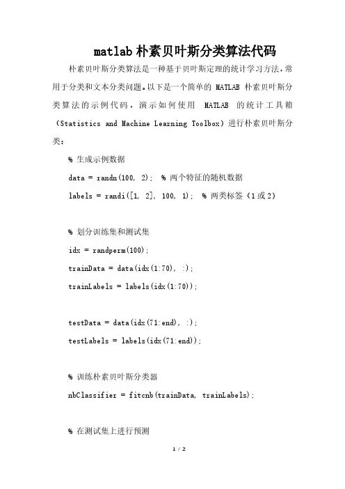
matlab朴素贝叶斯分类算法代码朴素贝叶斯分类算法是一种基于贝叶斯定理的统计学习方法,常用于分类和文本分类问题。
以下是一个简单的 MATLAB 朴素贝叶斯分类算法的示例代码,演示如何使用MATLAB 的统计工具箱(Statistics and Machine Learning Toolbox)进行朴素贝叶斯分类:% 生成示例数据data = randn(100, 2); % 两个特征的随机数据labels = randi([1, 2], 100, 1); % 两类标签(1或2)% 划分训练集和测试集idx = randperm(100);trainData = data(idx(1:70), :);trainLabels = labels(idx(1:70));testData = data(idx(71:end), :);testLabels = labels(idx(71:end));% 训练朴素贝叶斯分类器nbClassifier = fitcnb(trainData, trainLabels);% 在测试集上进行预测predictedLabels = predict(nbClassifier, testData);% 评估分类器性能accuracy = sum(predictedLabels == testLabels) / numel(testLabels);disp(['分类器准确率:', num2str(accuracy * 100), '%']);这个例子中,我们首先生成了一些随机的二维数据,并为每个数据点分配了一个类标签。
然后,我们将数据分为训练集和测试集。
接着,使用 fitcnb 函数训练朴素贝叶斯分类器,并使用 predict 函数在测试集上进行预测。
最后,计算分类器的准确率。
请注意,这只是一个简单的演示,实际应用中你可能需要更复杂的数据集和特征工程。

enter_evidence是MATLAB 中贝叶斯网络工具箱(Bayesian Network Toolbox)的一个函数。
这个函数的主要作用是将观测数据(即证据)添加到贝叶斯网络中,用于后续的概率推理或学习。
贝叶斯网络是一个概率图模型,其中随机变量之间的依赖关系通过一个有向无环图来表示。
在使用enter_evidence函数时,通常的用法是将证据数据作为参数传递给该函数,然后这些数据将被添加到贝叶斯网络中。
函数的基本语法如下:
net = enter_evidence(net, evidence)
其中:
●net是一个贝叶斯网络对象。
●evidence是一个结构体数组,其中每个结构体表示一个观察到的随机变量
的值。
例如,假设你有一个包含两个随机变量的贝叶斯网络,变量名为A和B。
如果你观察到A的值为1,你可以使用以下代码将这个观察值添加到网络中:net = enter_evidence(net, struct('A', 1));
这个操作之后,所有依赖于A的父节点的概率更新将基于你提供的证据进行。
总的来说,enter_evidence函数在贝叶斯网络分析中起到了至关重要的作用,因为它允许用户根据观测数据更新网络的概率分布,这对于推理、预测和决策支持等任务是非常关键的。

如何使用贝叶斯网络工具箱2004-1-7版翻译:By 斑斑(QQ:23920620)联系方式:banban23920620@安装安装Matlab源码安装C源码有用的Matlab提示创建你的第一个贝叶斯网络手工创建一个模型从一个文件加载一个模型使用GUI创建一个模型推断处理边缘分布处理联合分布虚拟证据最或然率解释条件概率分布列表(多项式)节点Noisy-or节点其它(噪音)确定性节点Softmax(多项式 分对数)节点神经网络节点根节点高斯节点广义线性模型节点分类 / 回归树节点其它连续分布CPD类型摘要模型举例高斯混合模型PCA、ICA等专家系统的混合专家系统的分等级混合QMR条件高斯模型其它混合模型参数学习从一个文件里加载数据从完整的数据中进行最大似然参数估计先验参数从完整的数据中(连续)更新贝叶斯参数数据缺失情况下的最大似然参数估计(EM算法) 参数类型结构学习穷举搜索K2算法爬山算法MCMC主动学习结构上的EM算法肉眼观察学习好的图形结构基于约束的方法推断函数联合树消元法全局推断方法快速打分置信传播采样(蒙特卡洛法)推断函数摘要影响图 / 制定决策DBNs、HMMs、Kalman滤波器等等安装安装Matlab代码1.下载FullBNT.zip文件。
2.解压文件。
3.编辑"FullBNT/BNT/add_BNT_to_path.m"让它包含正确的工作路径。
4.BNT_HOME = 'FullBNT的工作路径';5.打开Matlab。
6.运行BNT需要Matlab版本在V5.2以上。
7.转到BNT的文件夹例如在windows下,键入8.>> cd C:\kpmurphy\matlab\FullBNT\BNT9.键入"add_BNT_to_path",执行这个命令。
添加路径。
添加所有的文件夹在Matlab的路径下。
10.键入"test_BNT",看看运行是否正常,这时可能产生一些数字和一些警告信息。
在试卷分析中应用贝叶斯网络初探冉兆春(海口经济学院,海南海口( 571127)摘要:考试成绩直接反映学生的学习效果,对学生成绩的分析是教师改进教学方式重要的参考依据。
本文利用贝叶斯网络建模,对影响学生成绩的几个因素进行统计分析,尝试给大数据时代的教学提供一种新的成绩分析方式,以供教师改进教学方式时参考。
关键词:成绩分析;贝叶斯网络;大数据;结构学习;参数学习中图分类号:G434 文献标识码:A 文章编号:2017(02)-Application of Bayesian Network in Papers AnalysisRAN Zhao-chun(Haikou College of Economics, Haikou, Hainan 571127)Abstract:Examination results directly reflect the students' learning effects, the analysis of student achievement is an important reference for teachers to improve teaching methods。
In this paper, Bayesian network modeling is used to conduct statistical analysis of several factors that affect students' performance and try to provide a new way of analyzing scores in teaching for the era of big data for reference when teachers improve their teaching methods.Key words: performance analysis; Bayesian network; big data; structure learning; parameter learning考试是教学过程中的重要一环,试卷分析是检查教学成果、检讨教学手段的必要手段,以往多是依靠教师的主观经验来分析和判断,在客观全面和分析深度上受教师的个人水平和经验的限制,差异很大。

在MATLAB中使用贝叶斯统计方法的技巧介绍贝叶斯统计方法是一种强大的分析工具,它基于贝叶斯定理,能够通过更新先验知识来进行概率推理。
在许多领域中,贝叶斯统计方法已经得到广泛应用。
而在MATLAB中使用贝叶斯统计方法也相对容易,本文将介绍一些在MATLAB中使用贝叶斯统计方法的技巧。
贝叶斯定理在深入探讨贝叶斯统计方法之前,我们需要先了解贝叶斯定理。
贝叶斯定理是一个基于条件概率的公式,用于计算在给定某些先验知识的情况下,根据新的证据更新概率。
贝叶斯定理的公式可以表示为:P(A|B) = (P(B|A) * P(A)) / P(B)其中,P(A|B)表示在给定B的条件下A的概率,P(B|A)表示在给定A的条件下B的概率,P(A)和P(B)分别表示A和B的先验概率。
贝叶斯定理展示了如何将先验知识与新证据相结合,从而得到后验概率。
后验概率表示在考虑先验知识和新证据的情况下,某个事件发生的概率。
贝叶斯统计方法的优势使用贝叶斯统计方法有许多优势。
其中之一是能够有效地利用先验知识,从而更准确地推断结果。
贝叶斯统计方法还允许将不确定性以概率的形式进行建模,这对于实际问题的分析非常有帮助。
在MATLAB中使用贝叶斯统计方法的步骤使用贝叶斯统计方法在MATLAB中进行分析通常需要以下步骤:1. 收集数据:首先,需要收集实验数据或观测数据。
这些数据将用于提取统计模型的参数。
2. 建立模型:根据问题的特点和目标,选择合适的概率模型来描述数据的分布特征。
常见的概率模型包括高斯分布和泊松分布等。
3. 选择先验分布:在贝叶斯统计方法中,需要选择先验分布。
先验分布是在考虑任何观测数据之前对参数的主观假设。
根据实际问题和领域知识,选择合适的先验分布。
4. 计算后验分布:在获得观测数据之后,利用贝叶斯定理计算后验分布。
在MATLAB中,可以使用贝叶斯统计工具箱中的函数来计算后验分布。
5. 数据分析和推断:根据后验分布,可以进行数据分析和推断。
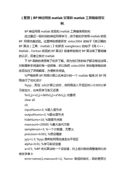
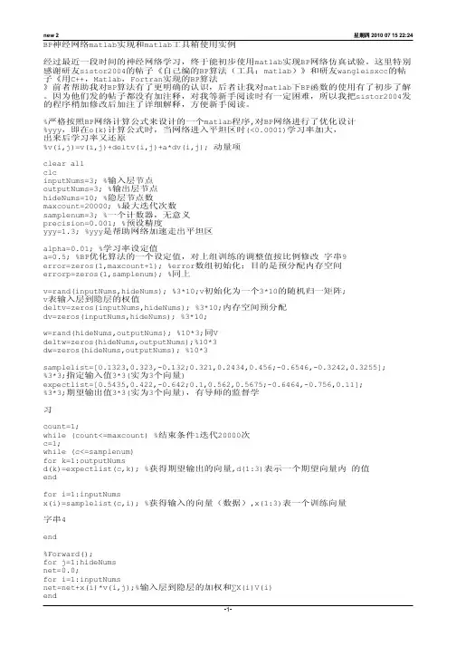
(整理)BP神经网络matlab实现和matlab工具箱使用实例.BP神经网络matlab实现和matlab工具箱使用实例经过最近一段时间的神经网络学习,终于能初步使用matlab实现BP网络仿真试验。
这里特别感谢研友sistor2004的帖子《自己编的BP算法(工具:matlab)》和研友wangleisxcc的帖子《用C++,Matlab,Fortran实现的BP算法》前者帮助我对BP算法有了更明确的认识,后者让我对matlab下BP函数的使用有了初步了解。
因为他们发的帖子都没有加注释,对我等新手阅读时有一定困难,所以我把sistor2004发的程序稍加修改后加注了详细解释,方便新手阅读。
%严格按照BP网络计算公式来设计的一个matlab程序,对BP网络进行了优化设计%yyy,即在o(k)计算公式时,当网络进入平坦区时(<0.0001)学习率加大,出来后学习率又还原%v(i,j)=v(i,j)+deltv(i,j)+a*dv(i,j); 动量项clear allclcinputNums=3; %输入层节点outputNums=3; %输出层节点hideNums=10; %隐层节点数maxcount=20000; %最大迭代次数samplenum=3; %一个计数器,无意义precision=0.001; %预设精度yyy=1.3; %yyy是帮助网络加速走出平坦区alpha=0.01; %学习率设定值a=0.5; %BP优化算法的一个设定值,对上组训练的调整值按比例修改字串9error=zeros(1,maxcount+1); %error数组初始化;目的是预分配内存空间errorp=zeros(1,samplenum); %同上v=rand(inputNums,hideNums); %3*10;v初始化为一个3*10的随机归一矩阵; v表输入层到隐层的权值deltv=zeros(inputNums,hideNums); %3*10;内存空间预分配dv=zeros(inputNums,hideNums); %3*10;w=rand(hideNums,outputNums); %10*3;同Vdeltw=zeros(hideNums,outputNums);%10*3dw=zeros(hideNums,outputNums); %10*3samplelist=[0.1323,0.323,-0.132;0.321,0.2434,0.456;-0.6546,-0.3242,0.3255]; %3*3;指定输入值3*3(实为3个向量)expectlist=[0.5435,0.422,-0.642;0.1,0.562,0.5675;-0.6464,-0.756,0.11]; %3*3;期望输出值3*3(实为3个向量),有导师的监督学习count=1;while (count<=maxcount) %结束条件1迭代20000次c=1;while (c<=samplenum)for k=1:outputNumsd(k)=expectlist(c,k); %获得期望输出的向量,d(1:3)表示一个期望向量内的值endfor i=1:inputNumsx(i)=samplelist(c,i); %获得输入的向量(数据),x(1:3)表一个训练向量字串4end%Forward();for j=1:hideNumsnet=0.0;for i=1:inputNumsnet=net+x(i)*v(i,j);%输入层到隐层的加权和∑X(i)V(i)endy(j)=1/(1+exp(-net)); %输出层处理f(x)=1/(1+exp(-x))单极性sigmiod函数endfor k=1:outputNumsnet=0.0;for j=1:hideNumsnet=net+y(j)*w(j,k);endif count>=2&&error(count)-error(count+1)<=0.0001o(k)=1/(1+exp(-net)/yyy); %平坦区加大学习率else o(k)=1/(1+exp(-net)); %同上endend%BpError(c)反馈/修改;errortmp=0.0;for k=1:outputNumserrortmp=errortmp+(d(k)-o(k))^2; %第一组训练后的误差计算enderrorp(c)=0.5*errortmp; %误差E=∑(d(k)-o(k))^2 * 1/2%end%Backward();for k=1:outputNumsyitao(k)=(d(k)-o(k))*o(k)*(1-o(k)); %输入层误差偏导字串5endfor j=1:hideNumstem=0.0;for k=1:outputNumstem=tem+yitao(k)*w(j,k); %为了求隐层偏导,而计算的∑endyitay(j)=tem*y(j)*(1-y(j)); %隐层偏导end%调整各层权值for j=1:hideNumsfor k=1:outputNumsdeltw(j,k)=alpha*yitao(k)*y(j); %权值w的调整量deltw(已乘学习率)w(j,k)=w(j,k)+deltw(j,k)+a*dw(j,k);%权值调整,这里的dw=dletw(t-1),实际是对BP算法的一个dw(j,k)=deltw(j,k); %改进措施--增加动量项目的是提高训练速度endendfor i=1:inputNumsfor j=1:hideNumsdeltv(i,j)=alpha*yitay(j)*x(i); %同上deltwv(i,j)=v(i,j)+deltv(i,j)+a*dv(i,j);dv(i,j)=deltv(i,j);endendc=c+1;end%第二个while结束;表示一次BP训练结束double tmp;tmp=0.0; 字串8for i=1:samplenumtmp=tmp+errorp(i)*errorp(i);%误差求和endtmp=tmp/c;error(count)=sqrt(tmp);%误差求均方根,即精度if (error(count)<precision)%另一个结束条件< p="">break;endcount=count+1;%训练次数加1end%第一个while结束error(maxcount+1)=error(maxcount);p=1:count;pp=p/50;plot(pp,error(p),"-"); %显示误差然后下面是研友wangleisxcc的程序基础上,我把初始化网络,训练网络,和网络使用三个稍微集成后的一个新函数bpnet %简单的BP神经网络集成,使用时直接调用bpnet就行%输入的是p-作为训练值的输入% t-也是网络的期望输出结果% ynum-设定隐层点数一般取3~20;% maxnum-如果训练一直达不到期望误差之内,那么BP迭代的次数一般设为5000% ex-期望误差,也就是训练一小于这个误差后结束迭代一般设为0.01% lr-学习率一般设为0.01% pp-使用p-t虚拟蓝好的BP网络来分类计算的向量,也就是嵌入二值水印的大组系数进行训练然后得到二值序列% ww-输出结果% 注明:ynum,maxnum,ex,lr均是一个值;而p,t,pp,ww均可以为向量字串1% 比如p是m*n的n维行向量,t那么为m*k的k维行向量,pp为o*i的i维行向量,ww为o* k的k维行向量%p,t作为网络训练输入,pp作为训练好的网络输入计算,最后的ww作为pp经过训练好的BP训练后的输出function ww=bpnet(p,t,ynum,maxnum,ex,lr,pp)plot(p,t,"+");title("训练向量");xlabel("P");ylabel("t");[w1,b1,w2,b2]=initff(p,ynum,"tansig",t,"purelin"); %初始化含一个隐层的BP网络zhen=25; %每迭代多少次更新显示biglr=1.1; %学习慢时学习率(用于跳出平坦区)litlr=0.7; %学习快时学习率(梯度下降过快时)a=0.7 %动量项a大小(△W(t)=lr*X*ん+a*△W(t-1))tp=[zhen maxnum ex lr biglr litlr a 1.04]; %trainbpx[w1,b1,w2,b2,ep,tr]=trainbpx(w1,b1,"tansig",w2,b2,"purelin", p,t,tp);ww=simuff(pp,w1,b1,"tansig",w2,b2,"purelin"); %ww就是调用结果下面是bpnet使用简例:%bpnet举例,因为BP网络的权值初始化都是随即生成,所以每次运行的状态可能不一样。
MATLAB网络分析与建模工具箱的使用指南引言网络分析与建模是现代科学中的一个重要的研究领域,它涉及到社交网络、电力系统、交通网络等许多应用领域。
MATLAB是一个功能强大的数值计算工具,其网络分析与建模工具箱提供了一系列用于分析和建模网络的函数和工具。
本文将针对MATLAB网络分析与建模工具箱进行详细介绍和使用指南。
一、网络分析基础知识在开始学习MATLAB网络分析与建模工具箱之前,我们需要了解一些网络分析的基础知识。
网络是由节点和边组成的图形结构,其中节点表示网络中的个体,边表示节点之间的关系。
节点和边可以是任意类型的,比如人物、电力站和电缆等。
网络分析常用的概念包括节点的度、网络的直径、节点的邻居等。
节点的度指的是与该节点相连的边的数量,可以用来度量节点的重要性或者中心性。
网络的直径则是网络中任意两个节点之间最短路径的最大长度,用来度量网络的连通性。
节点的邻居是指与该节点直接相连的其他节点。
二、MATLAB网络分析与建模工具箱的安装与导入要使用MATLAB网络分析与建模工具箱,首先需要从MathWorks官方网站下载并安装MATLAB软件。
安装完成后,我们可以在MATLAB命令窗口输入以下命令导入网络分析与建模工具箱:```MATLABaddpath(genpath('toolbox/nnet'));```导入成功后,我们就可以开始使用网络分析与建模工具箱进行分析和建模了。
三、网络的创建和可视化在MATLAB中,我们可以使用网络对象来表示和操作网络。
网络对象是网络分析与建模工具箱中的一个重要数据类型,它可以包含节点和边的信息,并且提供了一系列函数来进行网络的创建和操作。
要创建一个网络对象,我们可以使用以下命令:```MATLABnet = network;```创建好网络对象后,我们可以通过添加节点和边来构建网络。
使用以下命令可以添加节点:```MATLABnet = addnode(net, numNodes);```其中,numNodes是要添加的节点数量。
贝叶斯优化是一种优化方法,通常用于调整模型参数以提高模型在特定任务上的性能。
在深度学习中,长短期记忆网络(LSTM)是一种常用的循环神经网络结构,用于处理序列数据和时间序列数据。
在实际应用中,调整LSTM模型的参数对于模型性能的提升至关重要。
而使用贝叶斯优化方法来调整LSTM模型的参数,则可以更加高效地找到最优的参数组合,从而提高模型性能。
而在实际应用中,Matlab是一种常用的科学计算软件,具有强大的数学建模和仿真能力。
结合贝叶斯优化和Matlab工具,可以快速而有效地调整LSTM模型的参数,以获得更好的性能。
接下来,我们将以贝叶斯优化LSTM参数在Matlab中的实践为主题,探讨如何使用贝叶斯优化方法来调整LSTM模型的参数,以及如何在Matlab环境中实现这一方法。
一、贝叶斯优化方法概述贝叶斯优化是一种基于贝叶斯理论的优化方法,它通过不断地在候选参数空间中选择新的参数组合,并观察这些参数组合对目标函数的影响,从而逐步收敛到最优的参数组合。
在贝叶斯优化中,模型参数的选择是基于对参数空间的建模,通过对参数空间进行高效的探索和利用,以更快地找到最优解。
二、LSTM模型参数调整的重要性LSTM作为一种能够有效处理序列数据的循环神经网络结构,在许多应用中都取得了良好的效果。
然而,LSTM模型的性能往往受到模型参数的选择和调整的影响。
对LSTM模型的参数进行调整,以使其更好地适应特定的任务和数据,是至关重要的。
三、贝叶斯优化LSTM参数在Matlab中的实践在Matlab中,可以使用贝叶斯优化工具箱(Bayesian Optimization Toolbox)来实现LSTM参数的优化调整。
需要定义LSTM模型的目标函数,即需要优化的性能指标。
通常情况下,可以选择模型的准确率、损失函数值或其他相关的评价指标作为目标函数。
通过定义模型参数的候选空间和参数的先验分布,将LSTM模型的参数调整问题转化为一个贝叶斯优化问题。
MATLAB工具箱的应用实例与推荐引言:作为一种常用的科学计算软件,MATLAB拥有广泛的工具箱(Toolbox),涵盖了多个领域的专业功能与算法。
本文将介绍几个常用的MATLAB工具箱的应用实例,并推荐一些适合特定需求的工具箱。
一、信号与图像处理工具箱(Signal Processing Toolbox)信号与图像处理工具箱是MATLAB中常用的一个工具箱,它提供了丰富的信号分析和处理函数,能够帮助用户进行信号预处理、滤波、频谱分析等操作。
以下是一个应用实例:实例:心电信号分析在医学领域,心电信号分析是一项重要的研究工作。
使用信号与图像处理工具箱,我们可以通过MATLAB对心电信号进行处理与分析。
首先,可以使用滤波函数对心电信号进行降噪处理,去除不相关的干扰。
接下来,可以利用频谱分析函数,对心电信号进行频域分析,以了解信号的频谱特性。
在结合其他相关算法与方法后,我们可以进一步对心电信号进行心律失常检测、心脏疾病预测等工作。
推荐工具箱:除了信号与图像处理工具箱,在特定的领域和任务中,不同的工具箱也能够提供专门的功能与算法支持。
接下来,将为一些常见的应用领域介绍适用的MATLAB工具箱。
二、控制系统工具箱(Control System Toolbox)控制系统工具箱是专门针对控制系统设计与分析的一个工具箱,它提供了丰富的线性与非线性控制系统函数。
以下是一个应用实例:实例:PID控制器设计在工业自动化过程中,PID(Proportional-Integral-Derivative)控制器是一种常见的控制器类型。
使用控制系统工具箱,我们可以通过MATLAB设计与调整PID 控制器的参数。
首先,可以利用系统建模函数,对被控对象进行建模与参数估计。
接下来,可以使用PID自动调参函数,对PID控制器进行参数优化。
最后,通过对控制系统进行仿真与实时实验,可以验证与评估控制器的性能。
三、优化工具箱(Optimization Toolbox)优化工具箱提供了多种优化算法与函数,用于在数学模型中寻找最优解或近似最优解。