计算流体力学(CFD)文档——8. Turbulence modelling

计算流体动力学分析-CFD软件原理与应用_王福军--阅读笔记计算流体动力学(简称CFD)是建立在经典流体动力学与数值计算方法基础之上的一门新型独立学科，通过计算机数值计算和图像显示的方法，在时间和空间上定量描述流场的数值解，从而达到对物理问题研究的目的。

它兼有理论性和实践性的双重特点。

第一章节流体流动现象大量存在于自然界及多种工程领域中，所有这些过程都受质量守恒、动量守恒和能量守恒等基本物理定律的支配。

本章向读者介绍这些守恒定律的数学表达式，在此基础上提出数值求解这些基本方程的思想，阐述计算流体力学的任务及相关基础知识，最后简要介绍目前常用的计算流体动力学商用软件。

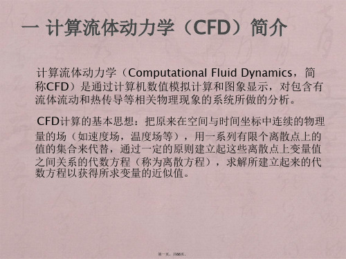
计算流体动力学((Computational Fluid Dynamics简称CFD)是通过计算机数值计算和图像显示，对包含有流体流动和热传导等相关物理现象的系统所做的分析。

CFD的基本思想可以归结为:把原来在时间域及空间域上连续的物理量的场，如速度场和压力场，用一系列有限个离散点上的变量值的集合来代替，通过一定的原则和方式建立起关于这些离散点上场变量之间关系的代数方程组，然后求解代数方程组获得场变量的近似值。

CFD可以看做是在流动基本方程(质量守恒方程、动量守恒方程、能量守恒方程)控制卜对流动的数值模拟。

通过这种数值模拟，我们可以得到极其复杂问题的流场内各个位置上的基本物理量(如速度、压力、温度、浓度等)的分布，以及这些物理量随时间的变化情况，确定旋涡分布特性、空化特性及脱流区等。

还可据此算出相关的其他物理量，如旋转式流体机械的转矩、水力损失和效率等。

此外，与CAD联合，还可进行结构优化设计等。

1.1.2计算流体动力学的工作步骤采用CFD的方法对流体流动进行数值模拟，通常包括如下步骤:(1)建立反映工程问题或物理问题本质的数学模型。

具体地说就是要建立反映问题各个量之间关系的微分方程及相应的定解条件，这是数值模拟的出发点。

没有正确完善的数学模型，数值模拟就毫无意义。

计算流体力学典型算例流体力学是研究液体和气体在运动中的力学性质和行为的学科。

计算流体力学（CFD）是一种利用数学模型和数值方法来模拟和解决流体力学问题的技术。

在实际应用中，CFD被广泛应用于工程、航空航天、天气预报等领域。

下面将介绍一个典型的计算流体力学算例。

典型算例：空气动力学性能分析假设我们要研究一架新型飞机的空气动力学性能，我们可以利用CFD来模拟和计算该飞机在不同速度和攻角条件下的气动特性。

首先，我们需要建立飞机的几何模型。

这可以通过计算机辅助设计（CAD）软件来完成，将飞机的几何形状和细节信息输入到CFD软件中。

接下来，我们需要为计算设置边界条件。

边界条件包括飞机表面的边界条件和远场环境的边界条件。

在飞机表面，我们可以设置壁面条件和粘性条件。

远场环境的边界条件可以设置为自由流条件，即远离飞机的区域中的流体速度和压力。

然后，我们可以选择适当的数值方法来求解流体力学方程。

CFD软件通常提供了多种数值方法，如有限体积法、有限元法和谱方法等。

根据实际情况，我们可以选择合适的数值方法来模拟飞机周围的流场。

接下来，我们需要设置求解参数。

这些参数包括时间步长、网格大小、迭代收敛准则等。

根据计算资源和精度要求，我们可以选择合适的参数值。

完成设置后，我们可以开始进行计算。

CFD软件将根据初始条件和边界条件，以迭代方式求解流体力学方程。

每一步迭代都会更新飞机周围的流场，直到达到收敛标准。

计算完成后，我们可以通过CFD软件提供的可视化工具来分析计算结果。

我们可以查看飞机周围的流线、压力分布、速度分布等信息，并进一步分析飞机的气动特性，如升力系数、阻力系数等。

通过这个典型算例，我们可以看到CFD在空气动力学性能分析中的应用。

CFD技术可以快速、准确地模拟复杂流体力学问题，并提供详细的结果分析。

这使得CFD成为现代工程设计和优化中不可或缺的工具。

计算流体力学作业答案问题1：什么是计算流体力学？计算流体力学（Computational Fluid Dynamics，简称CFD）是研究流体力学问题的一种方法，它使用数值方法对流体流动进行数值模拟和计算。

主要包括求解流体运动的方程组，通过空间离散和时间积分等计算方法，得到流体在给定条件下的运动和相应的物理量。

问题2：CFD的应用领域有哪些？CFD的应用领域非常广泛，包括但不限于以下几个方面：1.汽车工业：CFD可以用于汽车流场的模拟和优化，包括空气动力学性能和燃烧过程等。

2.航空航天工业：CFD可以用于飞机、火箭等流体动力学性能的预测和优化，包括机身、机翼的设计和改进等。

3.能源领域：CFD可以用于燃烧、热交换等能源领域的流体力学问题求解和优化。

4.管道流动：CFD可以用于石油、化工等行业的管道流动模拟和流体输送优化。

5.空气净化：CFD可以用于大气污染物的传输和分布模拟，以及空气净化设备的设计和改进。

6.生物医药：CFD可以用于生物流体输送和生物反应过程的模拟和分析，包括血液流动、药物输送等。

问题3：CFD的数值方法有哪些？CFD的数值方法一般包括以下几种：1.有限差分法（Finite Difference Method，FDM）：将模拟区域划分为网格，并在网格上离散化流体运动的方程组，利用有限差分近似求解。

2.有限体积法（Finite Volume Method，FVM）：将模拟区域划分为有限体积单元，通过对流体流量和通量的控制方程进行离散化，求解离散化方程组。

3.有限元法（Finite Element Method，FEM）：将模拟区域划分为有限元网格，通过对流体运动方程进行弱形式的变分推导，将流动问题转化为求解线性方程组。

4.谱方法（Spectral Method）：采用谱方法可以对流体运动方程进行高精度的空间离散，通常基于傅里叶变换或者基函数展开的方式进行求解。

5.计算网格方法（Meshless Methods）：不依赖网格的数值方法，主要包括粒子方法（Particle Methods）、网格自适应方法（Gridless Method）等。

计算流体力学的数学模型与方法计算流体力学（Computational Fluid Dynamics，简称CFD）是研究流体运动的力学现象而采用的计算方法。

它结合了数学模型和计算方法，通过数值计算和模拟的手段，来解决流体问题。

本文将从数学模型和计算方法两个方面，探讨计算流体力学的基本原理与应用。

一、数学模型数学模型是计算流体力学的基础，它描述了流体运动的基本方程和边界条件。

常用的数学模型包括Navier-Stokes方程、动量守恒方程、质量守恒方程和能量守恒方程等。

1. Navier-Stokes方程Navier-Stokes方程是描述流体的速度和压力随时间和空间变化的方程。

其一般形式为：\[\frac{\partial \rho}{\partial t} + \nabla \cdot (\rho \mathbf{v}) = 0\]其中，$\rho$表示流体的密度，$\mathbf{v}$表示流体的速度。

2. 动量守恒方程动量守恒方程描述了流体运动中动量的变化。

它可以表示为：\[\frac{\partial (\rho \mathbf{v})}{\partial t} + \nabla \cdot (\rho\mathbf{v} \mathbf{v}) = -\nabla p + \nabla \cdot \mathbf{\tau}\]其中，$p$表示压力，$\mathbf{\tau}$表示粘性应力张量。

3. 质量守恒方程质量守恒方程描述了流体质量的守恒。

它可以表示为：\[\frac{\partial \rho}{\partial t} + \nabla \cdot (\rho \mathbf{v}) = 0\]4. 能量守恒方程能量守恒方程描述了流体能量的守恒。

它可以表示为：\[\frac{\partial (\rho e)}{\partial t} + \nabla \cdot (\rho e \mathbf{v}) =\nabla \cdot (\lambda \nabla T) + \nabla \cdot (\mathbf{\tau \cdot v}) + \rho \mathbf{v} \cdot \mathbf{g}\]其中，$e$表示单位质量流体的总能量，$T$表示温度，$\lambda$表示热导率。

应用计算流体力学计算流体力学（Computational Fluid Dynamics，简称CFD）是一种研究流体力学现象的数值计算方法。

它通过将流体力学方程离散化为数值计算模型，利用计算机对这些模型进行求解，从而得到流体力学问题的数值解。

CFD在航空航天、汽车工程、能源、环境保护等领域具有广泛应用。

在航空航天领域，应用CFD可以对飞机的气动性能进行预测和优化。

通过对飞机的外形进行数值模拟，可以得到飞机在不同飞行状态下的升力、阻力、升阻比等气动参数。

这些参数对于飞机设计和气动外形优化具有重要意义，能够提高飞机的飞行性能和燃油经济性。

在汽车工程领域，应用CFD可以对车辆的空气动力学特性进行研究。

通过对车辆周围流场的模拟，可以得到车辆在行驶过程中的空气阻力、升力和气动稳定性等参数。

这些参数对于车辆的外形设计和空气动力学优化具有重要作用，能够提高车辆的行驶稳定性和燃油经济性。

在能源领域，应用CFD可以对风力发电机组的性能进行评估和优化。

通过对风力发电机组周围流场的模拟，可以得到风力对叶片的作用力、风力发电机组的输出功率和效率等参数。

这些参数对于风力发电机组的设计和功率提升具有重要意义，能够提高风力发电的利用效率和经济性。

在环境保护领域，应用CFD可以对大气污染物的传输和扩散进行模拟和预测。

通过对大气流场的模拟，可以得到污染物在大气中的传输路径、浓度分布和扩散范围等信息。

这些信息对于环境污染的防治和环境影响评价具有重要意义，能够提供科学依据和决策支持。

除了上述领域，CFD还广泛应用于船舶工程、石油工程、化工工程、建筑设计等领域。

通过CFD的应用，可以对流体力学现象进行深入分析和理解，为工程设计和科学研究提供有力的支持。

然而，CFD也存在一些挑战和限制。

首先，CFD模拟的结果受到多个参数和假设的影响，需要对模型和边界条件进行合理选择和验证。

其次，CFD计算过程需要大量的计算资源和时间，对计算机性能和算法效率有较高要求。

7. TURBULENCE SPRING 2011 7.1 What is turbulence?7.2 Momentum transfer in laminar and turbulent flow7.3 Turbulence notation7.4 Effect of turbulence on the mean flow7.5 Turbulence generation and transport7.6 Important shear flowsSummaryExamplesPART (a) – THE NATURE OF TURBULENCE7.1 What is Turbulence?• A “random”, 3-d, time-dependent eddying motion with many scales, superposed on an often drastically simpler mean flow.• A solution of the Navier-Stokes equations.•The natural state at high Reynolds numbers.•An efficient transporter and mixer ... of momentum, energy, constituents.• A major source of energy loss.• A significant influence on drag and boundary-layer separation.•“The last great unsolved problem of classical physics.” (variously attributed to Sommerfeld, Einstein and Feynman)7.2 Momentum Transfer in Laminar and Turbulent Flow In laminar flow adjacent layers of fluid slide past each other without mixing . Transfer of momentum occurs between layers moving at different speeds because of viscous stresses .In turbulent flow adjacent layers continually mix. A net transfer of momentum occurs because of the mixing of fluid elements from layers with different mean velocity . This mixing is a far more effective means of transferring momentum than viscous stresses. Consequently, the mean-velocity profile tends to be more uniform in turbulent flow.7.3 Turbulence NotationThe instantaneous value of any flow variable can be decomposed into mean + fluctuation .mean + fluctuationMean and fluctuating parts are denoted by either:• an overbar and prime:u u u ′+= or • upper case and lower case: u U +The first is useful in deriving theoretical results but becomes cumbersome in general use. The notation being used is, hopefully, obvious from the context.By definition, the average fluctuation is zero:0=′uIn experimental work and in steady flow the “mean” is usually a time mean, whilst in theoretical work it is the probabilistic (or “ensemble”) mean. The process of taking the mean of a turbulent quantity or a product of turbulent quantities is called Reynolds averaging .The normal averaging rules for products apply: 222u u u ′+= (variance )v u v u uv ′′+= (covariance ) Thus, in turbulent flow the “mean of a product” is not equal to the “product of the means” but includes an (often significant) contribution from the net effect of turbulent fluctuations.laminar turbulent7.4 Effect of Turbulence on the Mean FlowEngineers are usually only interested in the mean flow. However, turbulence must still be considered because, although the averages of individual fluctuations (e.g. u ′ or v ′) are zero, the average of a product (e.g. v u ′′) is not and may lead to a significant net flux.Consider mass and momentum fluxes in the y direction across surface A . For simplicity, assume constant density.7.4.1 Continuity Mass flux: vAAverage mass flux:The only change is that the instantaneous velocity is replaced by the mean velocity.The mean velocity satisfies the same continuity equation as the instantaneous velocity .7.4.2 Momentumx -momentum flux:A uv u vA )()(= Average x -momentum flux: A v u v u u vA )()(′′+=The average momentum flux has the same form as the instantaneous momentum flux except for additional fluxes A v u ′′ due to the net effect of turbulent fluctuations. These additional terms arise because of the averaging of a product of fluctuating quantities.A net rate of transport of momentum A v u ′′ from lower to upper side of an interface ...• is equivalent to a net rate of transport of momentum A v u ′′− from upper to lower ; •has the same dynamic effect (i.e. same rate of transfer of momentum) as a stress (i.e. force per unit area) of v u ′′−.This apparent stress is called a Reynolds stress . In a fully-turbulent flow it is usually much larger than the viscous stress.Other Reynolds stresses (u u ′′−, v v ′′−, etc.) emerge when considering the flux of the different momentum components in different directions.In a simple shear flow the total stress is321stressturbulentstressviscousv u u′′−= (1)In fully-turbulent flow turbulent stress is usually substantially bigger than viscous stress.can be interpreted as either: • the apparent force (per unit area) exerted by the upper fluid on the lower, or • the rate of transport of momentum (per unit area) from upper fluid to lower. The dynamic effect – a transfer of momentum – is the same.The nature of the turbulent stress can be illustrated by considering the motion of particles whose fluctuating velocities allow them to cross an interface.If particle A migrates upward (v ′ > 0) then it tends to retain its original momentum, which is now lower than its surrounds (u ′ < 0). If particle B migrates downward (v ′ < 0) it tends to retain its original momentum which is now higher than its surrounds (u ′ > 0).In both cases, v u ′′− is positive and, on average , tends to reduce the momentum in the upper fluid or increase the momentum in the lowerfluid. Hence there is a net transfer of momentum from upper to lowerfluid, equivalent to the effect of an additional mean stress.Velocity FluctuationsNormal stresses : 222,,w v u ′′′ Shear stresses :v u u w w v ′′′′′′,,(In slightly careless, but extremely common, usage both v u ′′− and v u ′′ are referred to as“stresses”.)Most turbulent flows are anisotropic ; i.e. 222,,w v u ′′′ are different.Turbulent kinetic energy : )(22221w v u k ′+′+′=Turbulence intensity :UkUu itymean veloc ctuation square flu root-mean-rms32=′==y Uvu7.4.3 General ScalarIn general, the advection of any scalar quantity φ gives rise to an additional scalar flux in the mean-flow equations; e.g.321fluxadditional v v v φ′′+φ=φ (2)Again, the extra term is the result of averaging a product of fluctuating quantities.7.4.4 Turbulence ModellingAt high Reynolds numbers, turbulent fluctuations cause a much greater net momentum transfer than viscous forces throughout most of the flow. Thus, accurate modelling of the Reynolds stresses is vital.A turbulence model or turbulence closure is a means of approximating the Reynolds stresses (and other turbulent fluxes) in order to close the mean-flow equations. Section 8 will describe some of the commoner turbulence models used in engineering.7.5 Turbulence Generation and Transport7.5.1 Production and DissipationTurbulence is initially generated by instabilities in the flow caused by mean velocity gradients (e.g. ∂U /∂y ). These eddies in their turn breed new instabilities and hence smaller eddies. The process continues until the eddies become sufficiently small (and fluctuating velocity gradients ∂u i /∂x j sufficiently large) that viscous effects become significant and dissipate turbulence energy as heat.This process – the continual creation of turbulence energy at large scales, transfer of energy to smaller and smaller eddies and the ultimate dissipation of turbulence energy by viscosity – is called the turbulent energy cascade .7.5.2 Turbulent Transport EquationsIt is common experience that turbulence can be transported with the flow; (think of the turbulent wake behind a vehicle or downwind of a large building).It can be proved mathematically (Section 10 for MSc students) that:• Each Reynolds stress j i u u satisfies its own scalar-transport equation.• The source term for an individual Reynolds stress j i u u transport equation has the form:n dissipatio tion redistribu production source net −+=where:– production P ij is determined by mean velocity gradients ;– redistribution ij transfers energy between stresses via pressure fluctuations ; – dissipation ij involves viscosity acting on fluctuating velocity gradients.There are also “advection” terms (turbulence carried with the flow) and “diffusion” terms (if turbulent stresses vary from point to point).large eddiessmall eddies ENERGYCASCADEDISSIPA TION by viscosity•The production terms for different Reynolds stresses involve different mean velocity gradients; for example, the rate of production (per unit mass) of 211u u u ≡ anduv u u ≡21 are, respectively,)()()(21211z U vw y U vv x U vu z V uw y V uvxVuu P zUuw y U uv x U uu P ∂∂+∂∂+∂∂−∂∂+∂∂+∂∂−=∂∂+∂∂+∂∂−= (3)(Exercise : by “pattern-matching” write production terms for the other stresses).• Because:(i) mean velocity gradients are greater in some directions than others,(ii) motions in certain directions are selectively damped (e.g. by buoyancy forces orrigid boundaries),turbulence is usually anisotropic , i.e. 222,,w v u are all different.•In practice, most turbulence models do not actually solve transport equations for allturbulent stresses, but only for the turbulent kinetic energy )(22221w v u k ++=, relating the other stresses to this by an eddy-viscosity formula (see Section 8).7.6 Simple Shear FlowsA flow for which there is only one non-zero mean velocity gradient, ∂U/∂y, is called a simple shear flow. Because they form a good approximation to many real flows, have been extensively researched in the laboratory and are amenable to basic theory they are an important starting point for many turbulence models.For such a flow, the first of (3) and similar expressions show that P11 > 0 but that P22 = P33 = 0, and hence 2u tends to be the largest of the normal stresses because it is the only one with a non-zero production term. On the other hand, if there is a rigid boundary on y = 0 then it will selectively damp wall-normal fluctuations; hence 2v is the smallest of the normal stresses.If there are density gradients (for example in atmospheric or oceanic flows, in fires or near heated surfaces) then buoyancy forces will either damp (stable density gradient) or enhance (unstable density gradient) vertical fluctuations.7.6.1 Free FlowsMixing layerWake(plane or axisymmetric) Jet(plane or axisymmetric)U∆∆U∆u ui j∆u ui jFor these simple flows: • Maximum turbulence occurs where y U ∂∂/ is largest, because this is where turbulenceproduction occurs. Note, however, that in the case of wake or jet, some turbulence must have diffused into the central core, where 0/=∂∂y U . • uv has the opposite sign to ∂U /∂y and vanishes when this derivative vanishes.•These turbulent flows are anisotropic: 22v u >. This is because, for these simple shear flows, only the streamwise component has a production term:0,22211=∂∂−=P yUuv P7.6.2 Wall-Bounded FlowsPipe or channel flowFlat-plate boundary layerEven though the overall Reynolds number /Re L U ∞= may be large, and hence viscous transport much smaller than turbulent transport in the majority of the flow, there must be a thin layer very close to the wall where the local Reynolds number based on distance from the wall, /Re y u y =, is small and hence molecular viscosity is important.Wall UnitsAn important parameter is the wall shear stress w (drag per unit area). Like any other stress this has dimensions of [density] × [velocity]2 and hence it is possible to define an importantFrom u and it is possible to form a viscous length scale l = /u. Hence, we may defineu u i j constant-stress layerThe direct effects of molecular viscosity are usually only important when y + is O(1).The total mean shear stress is made up of viscous and turbulent parts:321321turbulentviscousuv −=When there is no streamwise pressure gradient is approximately constant over a significant depth and is equal to the wall stress w . This assumption of constant shear stress allows us to establish the velocity profile in regions where either viscous or turbulent stresses dominate.Viscous SublayerVery close to a smooth wall, turbulence is damped out by the presence of the boundary. In this region the shear stress is predominantly viscous. Assuming constant shear stress,w= ⇒ yU w = (6) i.e. the mean velocity profile in the viscous sublayer is linear . This is generally a good approximation in the range y + < 5.Log-Law RegionAt large Reynolds numbers, the turbulent part of the shear stress dominates throughout most of the boundary layer so that on dimensional grounds, since u and y are the only possible velocity and length scales,yuy U ∝∂∂ Integrating, and putting part of the constant of integration inside the logarithm (to make its argument dimensionless):)ln 1(B yu u U += (7)(von Kármán’s constant ) and B are universal constants with experimentally-determined values of about 0.41 and 5 respectively.Using the definition of wall units (equation (5)) these velocity profiles are often written inExperimental measurements indicate that the log law actually holds to a good approximation over a substantial proportion of the boundary layer. (This is where the logarithm originates in common friction-factor formulae such as the Colebrook-White formula for pipe flow). Consistency with the log law is probably the single most important consideration in the construction of turbulence models.•Turbulence is a 3-d, time-dependent, eddying motion with many scales, causing continuous mixing of fluid.•Each flow variable may be decomposed as mean + fluctuation.•The process of averaging turbulent variables or their products is called Reynolds averaging and leads to the Reynolds-averaged Navier-Stokes (RANS) equations.•Turbulent fluctuations make a net contribution to the transport of momentum and other quantities. Turbulence enters the mean momentum equations via the Reynolds stresses, e.g.vu turb ′′−=• A means of specifying the Reynolds stresses (and hence solving the mean flow equations) is called a turbulence model or turbulence closure.•Turbulence energy is generated at large scales by mean-velocity gradients (and, sometimes, body forces such as buoyancy). Turbulence is dissipated (as heat) at small scales by viscosity.•Because of the directional nature of the generating process (i.e. mean-velocity gradients and/or body forces) turbulence is initially anisotropic. Energy is subsequently redistributed amongst the different stress components by the action of pressure fluctuations and ultimately dissipated by the action of viscosity on the smallest scales.•Turbulence modelling is, to a large extent, guided by experimental observations and theoretical considerations for simple shear flows which may be free (e.g. mixing layer; jet; wake) or wall-bounded (e.g. pipe or channel flow; flat-plate boundary layer).Q1. Which is more viscous, air or water?Air:= 1.20 kg m –3 = 1.80×10–5 kg m –1 s –1 Water:= 1000 kg m –3 = 1.00×10–3 kg m –1 s –1Q2. The accepted critical Reynolds number in a round pipe (based on bulk velocity and diameter) is 2300. At what speed is this attained in 5-cm-diameter pipe for (a) air; (b) water?Q3. Sketch the mean velocity profile in a pipe at Reynolds numbers of (a) 500; (b) 50 000. What is the shear stress along the pipe axis in either case?Q4. Explain the process of flow separation. How does deliberately “tripping” a developing boundary layer help to prevent or delay separation on a convex curved surface?Q5. The following couplets are measured values of (u ,v ) in an idealised 2-d turbulent flow. Calculate u , v , 2u ′, 2v ′, v u ′′ from this set of numbers.(3.6,0.2) (4.1,–0.4) (5.2,–0.2) (4.6,–0.4) (3.4,0.0)(3.8,-0.4) (4.4,0.2) (3.9,0.4) (3.0,0.4) (4.4,–0.3) (4.0,-0.1) (3.4,0.1) (4.6,-0.2) (3.6,0.4) (4.0,0.3)Q6. The rate of production (per unit mass of fluid) of 2u and uv are, respectively,)(211z U uw y U uv x U uu P ∂∂+∂∂+∂∂−= )()(12zU vw y U vv x U vu z V uw y V uv x V uu P ∂∂+∂∂+∂∂−∂∂+∂∂+∂∂−=(a) By inspection, write down similar expressions for P 22, P 33, P 23, P 31, the rates ofproduction of 2v , 2w , vw and wu respectively.(b) Write down expressions for P 11, P 22, P 33 and P 12, P 23, P 31 in simple shear flow (where∂U /∂y is the only non-zero mean velocity gradient). What does this indicate about the relative distribution of turbulence energy amongst the various Reynolds-stress components? Write down also an expression for P (k ), the rate of production of turbulence kinetic energy.(c) A mathematician would summarise the different production terms by a compact formula)(ki k j k j k i ij x U u u x U u u P ∂∂+∂∂−= using the Einstein summation convention – implied summation over a repeated index (in this case, k ). See if you can relate this to the above expressions for the P ij .。