控制工程基础 南理工 HPWANG-FCE9
- 格式:pdf
- 大小:3.42 MB
- 文档页数:54


《控制工程基础》实验报告姓名欧宇涵 914000720206周竹青 914000720215 学院教育实验学院指导老师蔡晨晓南京理工大学自动化学院2017年1月实验1:典型环节的模拟研究一、实验目的与要求:1、学习构建典型环节的模拟电路;2、研究阻、容参数对典型环节阶跃响应的影响;3、学习典型环节阶跃响应的测量方法,并计算其典型环节的传递函数。
二、实验内容:完成比例环节、积分环节、比例积分环节、惯性环节的电路模拟实验,并研究参数变化对其阶跃响应特性的影响。
三、实验步骤与方法(1)比例环节图1-1 比例环节模拟电路图比例环节的传递函数为:K s U s U i O =)()(,其中12R RK =,参数取R 2=200K ,R 1=100K 。
步骤: 1、连接好实验台,按上图接好线。
2、调节阶跃信号幅值(用万用表测),此处以1V 为例。
调节完成后恢复初始。
3、Ui 接阶跃信号、Uo 接IN 采集信号。
4、打开上端软件,设置采集速率为“1800uS”,取消“自动采集”选项。
5、点击上端软件“开始”按键,随后向上拨动阶跃信号开关,采集数据如下图。
图1-2 比例环节阶跃响应(2)积分环节图1-3 积分环节模拟电路图积分环节的传递函数为:ST V V I I O 1-=,其中T I =RC ,参数取R=100K ,C=0.1µf 。
步骤:同比例环节,采集数据如下图。
图1-4 积分环节阶跃响应(3)微分环节图1-5 微分环节模拟电路图200KRV IVoC2CR 1V IVo200K微分环节的传递函数为:K S T S T V V D D I O +-=1,其中 T D =R 1C 、K=12R R。
参数取:R 1=100K ,R 2=200K ,C=1µf 。
步骤:同比例环节,采集数据如下图。
图1-6 微分环节阶跃响应(4)惯性环节图1-7 惯性环节模拟电路图惯性环节的传递函数为:1+-=TS K V V I O ,其中2T R C =,21RK R =-。

南理工控制工程基础实验报告成绩:《控制工程基础》课程实验报告班级:学号:姓名:南京理工大学2015年12月《控制工程基础》课程仿真实验一、已知某单位负反馈系统的开环传递函数如下G(s)?10 s2?5s?25借助MATLAB和Simulink完成以下要求:(1) 把G(s)转换成零极点形式的传递函数,判断开环系统稳定性。
>> num1=[10]; >> den1=[1 5 25]; >> sys1=tf(num1,den1) 零极点形式的传递函数:于极点都在左半平面,所以开环系统稳定。
(2) 计算闭环特征根并判别系统的稳定性,并求出闭环系统在0~10秒内的脉冲响应和单位阶跃响应,分别绘出响应曲线。
>> num=[10];den=[1,5,35]; >>sys=tf(num,den); >> t=[0::10]; >> [y,t]=step(sys,t); >> plot(t,y),grid >> xlabel(‘time(s)’) >> ylabel(‘output’) >> hold on; >> [y1,x1,t]=impulse(num,den,t); >> plot(t,y1,’:’),grid (3) 当系统输入r(t)?sin5t时,运用Simulink搭建系统并仿真,用示波器观察系统的输出,绘出响应曲线。
曲线:二、某单位负反馈系统的开环传递函数为:6s3?26s2?6s?20G(s)?4频率范围??[,100] s?3s3?4s2?2s?2 绘制频率响应曲线,包括Bode图和幅相曲线。
>> num=[6 26 6 20]; >> den=[1 3 4 2 2]; >> sys=tf(num,den); >> bode(sys,{,100}) >> grid on >> clear; >> num=[6 26 6 20]; >> den=[1 3 4 2 2]; >> sys=tf(num,den); >> [z , p , k] = tf2zp(num, den); >> nyquist(sys) 根据Nyquist判据判定系统的稳定性。

实验1 模拟控制系统在阶跃响应下的特性实验一、实验目的根据等效仿真原理,利用线性集成运算放大器及分立元件构成电子模拟器,以干电池作为输入信号,研究控制系统的阶跃时间响应。
二、实验内容研究一阶与二阶系统结构参数的改变,对系统阶跃时间响应的影响。
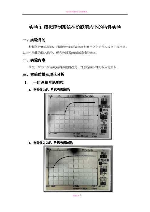
三、实验结果及理论分析1.一阶系统阶跃响应a.电容值1uF,阶跃响应波形:b.电容值2.2uF,阶跃响应波形:c. 电容值4.4uF ,阶跃响应波形:2. 一阶系统阶跃响应数据表电容值 (uF ) 稳态终值U c (∞)(V )时间常数T(s)理论值实际值理论值实际值1.02.87 2.90 0.51 0.50 2.2 2.87 2.90 1.02 1.07 4.42.872.902.242.06元器件实测参数U r = -2.87VR o =505k ΩR 1=500k ΩR 2=496k Ω其中C R T 2=r c U R R U )/()(21-=∞误差原因分析:① 电阻值及电容值测量有误差; ② 干电池电压测量有误差; ③ 在示波器上读数时产生误差;④ 元器件引脚或者面包板老化,导致电阻变大; ⑤ 电池内阻的影响输入电阻大小。
⑥在C=4.4uF的实验中,受硬件限制,读数误差较大。
3.二阶系统阶跃响应a.阻尼比为0.1,阶跃响应波形:b.阻尼比为0.5,阶跃响应波形:c.阻尼比为0.7,阶跃响应波形:d.阻尼比为1.0,阶跃响应波形:4.二阶系统阶跃响应数据表ξR w(Ω)峰值时间t p(s)U o(t p)(V)调整时间t s(s)稳态终值U s(V)超调(%)M p震荡次数N0 .1454k0.3 4.8 2.8 2.9562.760 .552.9k0.4 3.30.5 2.9511.910 .724.6k0.4 3.00.3 2.92 2.711 .02.97k1.02.98 1.0 2.9800四、回答问题1.为什么要在二阶模拟系统中设置开关K1和K2,而且必须同时动作?答:K1的作用是用来产生阶跃信号,撤除输入信后,K2则是构成了C2的放电回路。

成绩:《控制工程基础》课程实验报告班级:11102002学号:1110200208姓名:汤国苑南京理工大学2013年12月《控制工程基础》课程仿真实验一、 已知某单位负反馈系统的开环传递函数如下 (25分)210()525G s s s =++ 借助MATLAB 和Simulink 完成以下要求:(1) 把G(s)转换成零极点形式的传递函数,判断开环系统稳定性。
MATLAB 程序: clear; num=[10]; den=[1 5 25]; sys=tf(num,den); [Z,P,K]=tf2zp(num,den)零极点形式的传递函数: )43301.05.2)(4401.45.2(10)(j s j s s G ++-+=由于极点均在左半平面,所以开环系统稳定。
(2) 计算闭环特征根并判别系统的稳定性,并求出闭环系统在0~10秒内的脉冲响应和单位阶跃响应,分别绘出响应曲线。
闭环传递函数 35510)(2++=s s s T特征方程355)(2++=s s s q 特征根 211551j s +-=211552j s --= 由于根在左半平面,所以系统稳定。
用simulink 仿真: 脉冲响应:结果:012345678910 -0.04-0.020.020.040.060.080.1仿真时间(s)幅值阶跃响应:结果:123456789100.050.10.150.20.250.30.350.4仿真时间(s )幅值(3) 当系统输入()sin5r t t 时,运用Simulink 搭建系统并仿真,用示波器观察系统的输出,绘出响应曲线。
曲线:二、 (25分)某单位负反馈系统的开环传递函数为:32432626620()3422s s s G s s s s s +++=++++ 频率范围[0.1,100]ω∈ (1) 绘制频率响应曲线,包括Bode 图和幅相曲线(Nyquist 图)。
Matlab 语句: clear;num=[6 26 6 20]; den=[1 3 4 2 2]; sys=tf(num,den); bode(sys,{0.1,100}) Bode 图:Matlab语句:clear;num=[6 26 6 20];den=[1 3 4 2 2];sys=tf(num,den);[z , p , k] = tf2zp(num, den) nyquist(sys)Nyquist图:(2)根据Nyquist判据判定系统的稳定性。
成绩:《控制工程基础》课程实验报告班级:111020021110200208 学号:姓名:汤国苑南京理工大学12月年20131《控制工程基础》课程仿真实验25分)已知某单位负反馈系统的开环传递函数如下(一、10?)G(s225ss??5 Simulink完成以下要求:借助MATLAB和转换成零极点形式的传递函数,判断开环系统稳定性。
把(1)G(s)程序:MATLABclear;num=[10];den=[1 5 25];sys=tf(num,den);[Z,P,K]=tf2zp(num,den)10零极点形式的传递函数:?s)(G).43301j?2.5?0j?(s2.5?4.4401)(s由于极点均在左半平面,所以开环系统稳定。
秒内的~10(2)计算闭环特征根并判别系统的稳定性,并求出闭环系统在0 脉冲响应和单位阶跃响应,分别绘出响应曲线。
10?s)T(闭环传递函数235?s?5s2特征方程35s)???5s(qs115?jj115?5?5?特征根?s?s2122由于根在左半平面,所以系统稳定。
用simulink仿真:脉冲响应:2阶跃响应:结果:3搭建系统并仿真,用示波器观Simulink当系统输入时,运用(3)t sin5)(rt察系统的输出,绘出响应曲线。
曲线:4(25分)某单位负反馈系统的开环传递函数为:二、??)G(s,100][0.1?频率范围2320?6?26ss6s?2342s?4?s?2?s3s。
Nyquist图)Bode1()绘制频率响应曲线,包括图和幅相曲线(Matlab语句:clear;num=[6 26 6 20];den=[1 3 4 2 2];sys=tf(num,den);bode(sys,{0.1,100})图:Bode52Matlab语句:clear;num=[6 26 6 20]; den=[1 3 4 2 2];sys=tf(num,den);[z , p , k] = tf2zp(num, den) nyquist(sys)图:Nyquist6判据判定系统的稳定性。
高纲1182江苏省高等教育自学考试大纲27481控制工程基础南京理工大学编江苏省高等教育自学考试委员会办公室一、课程性质及其设置目的与要求(一)课程性质和特点控制工程基础课程是江苏省高等教育自学考试电子工程专业本科段的必修的专业基础课,该课程是电子工程专业课程体系中的骨干课程之一。
控制工程基础知识在各个领域都有着广泛的应用,如航空航天系统、现代交通运输系统、管理决策系统、生产控制系统、机械控制系统、国防武器系统等等,是人们开发、利用信息传递以支持组织自动化生产,开发自动控制设备,是一门能极大地促进了现代社会组织的变革、推进了社会现代化进程、提高了组织自身素质与竞争能力的科学。
随着自动控制技术不断发展,自动控制技术这支利剑必须切实瞄准各行各业的业务需求这个目标,做到有的放矢,才能真正发挥作用。
控制工程基础这门课程的任务就是利用自动控制的理论及思想,结合具体实际情况,帮助学生掌握分析控制系统的性能及设计控制器的基本方法,从而提高学生理论水平,锻炼他们进行系统开发的能力,为将来从事实际工作奠定坚实的基础。
控制工程基础是一门系统性很强的应用型课程,是以讲解控制系统分析、设计及提高系统性能为主要内容,引导学生利用应用数学、力学、电子工程学等知识,不断深入理解控制工程相关知识、灵活运用知识的一门科学。
课程具有较强的理论性,学生通过具体的机械及电子控制系统的专门学习,在树立清晰的系统意识的基础上,掌握控制系统性能分析与系统设计的各种方法。
通过本课程的学习,学生不仅可以增强自学能力和独立研究能力,而且提高自身的开发能力,成为具备较强的研究能力、创新能力和驾驭现代化控制技术能力的复合型人才。
(二)本课程的基本要求通过本课程的学习,应达到如下要求:1.以机械运动作为主要控制对象,重点掌握数学模型及分析的基本思想和方法。
熟练掌握典型系统(特别是一阶系统、二阶系统)的时域和频域特性;2.重点掌握线性系统的性能指标的定义及意义,以及相应的求取思想和基本方法;3.重点掌握自动控制系统的稳定性的概念和常用的判定方法,能熟练应用基本的判定方法判别系统的稳定性;4.熟练掌握在典型输入信号作用下,系统的响应;4.熟练掌握控制系统建模的基本方法及模型简化的基本手段;5.掌握控制系统传递函数的概念,深刻理解传递函数性质及物理意义;6.掌握控制系统的设计思想和基本的方法;7.对基本的校正装置的作用有所了解。
Fundamentals of Control Engineering Ch9 Stability in the Frequency DomainHaoping WANG E-mail: Hp.wang@Automation SchoolNanjing University of Science and Technology Fundamentals of Control Engineering -hp.wang@j g y gyy q yCh9 Stability in the Frequency Domain IntroductionMapping contours in the s-planeNyquist CriterionRelative Stability and Nyquist CriterionTime-domain performance criteria specified in the Time-domain performance criteria specified in thefrequency domainStability of control System with time delaysFundamentals of Control Engineering -hp.wang@Introduction The frequency response of a system represents the sinusoidal steady-state response of a system and provides sufficient information for the state response of a system and provides sufficient information for the determination of the relative stability of the system.A f d i t bilit it i ll d N i t t bilit it i A frequency domain stability criterion called Nyquist stability criterion was developed by H. Nyquist in 1932.The Nyquist stability criterion is based on a theorem in the theory of the function of a complex variable due to Cauchy .The characteristic equation of the system isThe characteristic equation of the system is F(s) = 1 + L(s)where L(s) is a rational function of s .()To ensure stability, we must ascertain that all the zeros of F (s) lie in the left-hand s-plane. Nyquist thus proposed a mapping of the right-hand s-plane into the F(s)plane Fundamentals of Control Engineering -hp.wang@ plane into the F(s)-plane.y q yCh9 Stability in the Frequency Domain IntroductionMapping contours in the s-planeNyquist CriterionRelative Stability and Nyquist CriterionTime-domain performance criteria specified in the Time-domain performance criteria specified in thefrequency domainStability of control System with time delaysFundamentals of Control Engineering -hp.wang@A contours map is a contours or trajectory in one plane mapped or translated into another plane by a relation F(s)translated into another plane by a relation F(s).Since s is a complex variable, the function F(s) is itselfcomplex it can be defined as F(s)=u +j s j σω=+complex, it can be defined as F(s) = u + jv Exe 1. Let us consider a function F(s) = 2s + 1d t i th l h i Fi ()A di t th and a contours in the s-plane, as shown in Fig. (a). According to the relation ()2()1u jv F s j σω+==++we have21u σ=+⎧⎨The mapped contours in the F(s)-plane is shown in Fig 1. (b).2v ω=⎩Fundamentals of Control Engineering -hp.wang@21u σ=+⎧Fi 1M i t b F()2+12v ω⎨=⎩Fundamentals of Control Engineering -hp.wang@ Fig 1. Mapping a square contours by F(s) = 2s + 1.We assume clockwise traversal of a contour to be positive and the area enclosed within the contour to be on the right. and the area enclosed within the contour to be on the right Exe 2. Let us consider a rational function of sF(s) =s/(s + 2)Solution 2:Fundamentals of Control Engineering -hp.wang@Solution 2:Fig2. (a) square contour in the s-plane (b)and the resulting contour in the F(s)-planeFundamentals of Control Engineering -hp.wang@If the function F(s)is the characteristic equation, then we haven∏+()K s sCauchy’s theorem or Principle of the argument: If a contour Tin thess-plane encircles Z zeros and P poles of F(s) and does not pass through any poles or zeros of F(s) and the traversal is in the clockwise direction along the contour, the corresponding contour T F in the F(s)-plane encircles the origin of the F(s)-plane N = Z − P times in the clockwise direction.Fundamentals of Control Engineering -hp.wang@Exe 3. Let us consider the functionSolution 3: then we haveNow considering the vectors as shown for a specific contour T s in Fig.(a).Fundamentals of Control Engineering -hp.wang@Fi3E l ti f th t l f Fundamentals of Control Engineering -hp.wang@Fig 3: Evaluation of the net angle of T F.We can extend this case to a general case: If Z zeros and P poles are enclosed within T s , then the net angle would be equal to and, respectively.2z Z φπ=2p P φπ=If Z zeros and P poles are encircled as T s is traversed, then the net change angle of F(s)change angle of F(s) is22()F z p N Z P φφφππ=−⇒=−and the net number of encirclements of the origin of the F (s)-plane is −N Z P=Fundamentals of Control Engineering -hp.wang@Exe 4. Reflecting exampleFig 4Example of Cauchy’s theorem with three zeros and one pole within Completes two clockwise encirclements ofthe origin in the F(s)-planeFundamentals of Control Engineering -hp.wang@ Fig 4. Example of Cauchy s theorem with three zeros and one pole within T sExe 5. Reflecting exampleFig 5Example of Cauchy’s theorem with one pole within Completes one counterclockwise encirclementsof the origin in the F(s)-planeFundamentals of Control Engineering -hp.wang@ Fig 5. Example of Cauchy s theorem with one pole within T sy q yCh9 Stability in the Frequency Domain IntroductionMapping contours in the s-planeNyquist CriterionRelative Stability and Nyquist CriterionTime-domain performance criteria specified in the Time-domain performance criteria specified in thefrequency domainStability of control System with time delaysFundamentals of Control Engineering -hp.wang@Considering the characteristic equation, then we haven. The zeros of F(s) are the characteristic roots of the system Exe 6.Fundamentals of Control Engineering -hp.wang@Nyquist stability criterion(1) Choose the contour T s in the s-plane that enclosed the entire right-hand (1)Ch h i h l h l d h i i h h d s-plane, and we determine whether any zeros of F(s) lie within T s by utilizing Cauchy's theorem.(2) Plot the T F in the F(s) plane and determine the number of encirclementsgof the origin N;Then the number of zeros of F(s) within the T s contour (and therefore, the unstable zeros of F(s)) isZ N P=+Thus, if P= 0, as is usually the case, we find that the number of unstable Th if0i ll th fi d th t th b f t bl roots of the system is equal to N, the number of encirclements of the origin of the F(s)-plane.Fundamentals of Control Engineering -hp.wang@The Nyquist contour that encloses the entire right-hand s-plane is shown inFig 7.Fig 7.The Nyquist contour includes two parts:(1) The first part is the jw-axis from −infinityto +infinity ;y (2) The second part is the right semicircularpath with infinity radius r.Fig 7 Nyquist contour is shown as the heavy line.Fundamentals of Control Engineering -hp.wang@ g yqu st co tou s s o as t e ea y eThe Nyquist criterion is concerned with the mapping of the characteristic equationF (s) = 1 + L(s)(s)(s)and the number of encirclements of the origin .We may define the function :F’(s)=F(s)−1=L(s)We may define the function : F (s) F(s) 1 L(s)Then the mapping of T s in the s-plane will be through the function F’(s) = L(s) into the L(s)-plane.The number of clockwise encirclements of the origin of theF()l b th b f l k i i l t f th 1i t i th F(s)-plane becomes the number of clockwise encirclements of the −1 point in the L(s)-plane.case 1. A feedback system is stable if and only if the contour T L in the L(s)-plane does not encircle the (−1, 0) point when the number of poles of L(s) in the right-hand s-plane is zero (P = 0).case 2. A feedback system is stable if and only if, for the contour T L the number of counterclockwise encirclements of the (−1, 0) point is equal to the number of poles of L(s) with positive real parts.Fundamentals of Control Engineering -hp.wang@ 0Z PN P N =+=⇒=−Exe 8. Considering a system with 2 real poles K 121,1/10,100K ττ===Solution 8:12()(1)(1)L s s s ττ=++(1)+jw-axis -> solidcolored line;(2) The −jw-axis ->dashed colored line;(3) The semicirclewith r -> infinity ismapped into thei iFig 8Nyquist contour and mapping for GH(s)origin.Fundamentals of Control Engineering -hp.wang@ Fig 8. Nyquist contour and mapping for GH(s).Exe 9. Considering a system with a pole at origin()KGH s=s sτ+(1)g yq pp g()Fig 9. Nyquist contour and mapping for GH(s).Fundamentals of Control Engineering -hp.wang@Solution 9:()1)K L s s s τ=+()(1) The Portion from to . In this case, the contour T s is mapped by the functionL()|L(j )0ω+=ω=+∞L(s)|s=jw = L(jw)(2) The Portion from . In this case, the contour T s is to 0ωω−=−∞=plane In this case the mapping is represented by plane. In this case, the mapping is represented byFundamentals of Control Engineering -hp.wang@(4) The Origin of the s-plane . In Fig. 9, the small semicircular detour at the origin isdenoted as and to vary from -90°to +90°The mapping j φdenoted as and to vary from 90to +90. The mapping for GH(s) is,0s e εε=→φThus, the angle of the contour in the GH(s)-plane changes from +90°at to -90°at , passing through 0 at .0ω=0ω−=0ω+=Then using the Nyquist criterion, we obtain Z = N + P = 0 + 0 = 0, Thus the system is stableFundamentals of Control Engineering -hp.wang@There are three general conclusions from this example:g p(i)It is sufficient to construct the contour T L for the frequency rangein order to investigate the stability.0 ω+<<+∞(ii) The magnitude of L(s) as s = r.exp(j Ԅ) and r to infinity will normallyapproach zero or a constant.(iii)The contour T L for the small semicircular detour at the originalways starts at and ends at in the clockwise0ω+=0ω−=direction with infinity radius.The net angle change of the contour is , where v is the typev πg g yp number of L (s).Fundamentals of Control Engineering -hp.wang@Exe 10. system with 3 poles K L ==y p 12()()(1)(1)s GH s s s s ττ++Fundamentals of Control Engineering -hp.wang@Solution 10: The point where the GH(s)-locus intersects the real axis can be foundby setting the imaginary part of GH(jw)=u+jv equal to zero The transfer found by setting the imaginary part of GH(jw) u jv equal to zero. The transfer function GH(jw) can be decomposed asThen we haveThus,v=0when or .The magnitudeFundamentals of Control Engineering -hp.wang@ Thus, v 0 when or .The magnitudeof the real part of GH(jw) is thenTherefore, the system is stable whenConsider the case where , so thatUsing the further above relation, when K < 2, the system is stable.Fundamentals of Control Engineering -hp.wang@Fig: Nyquist diagrams forFundamentals of Control Engineering -hp.wang@Exe 11 (System with two poles at the origin). Consider a single-loop control system loop control system 2()1)K L s s s τ=+()According to Fig, we haveZ =N +P =2+0=2Z N + P 2 + 0 2Thus the system is unstable.Fundamentals of Control Engineering -hp.wang@Exe 12 (System with a pole in the right-hand s-plane). Consider a single-loop control system K 1()()(1)L s GH s s s ==−Fundamentals of Control Engineering -hp.wang@ Z=N+P=2, the system unstable Fig.12The Nyquist CriterionExe 13. Consider a open-loop control systemK1 (1 + K 2 s ) GH ( s ) = s ( s − 1)The GH(jw)-locus intersects the u-axis at a point u= −K1K2 (i) If −K1K2 < −1, the contour TGH encircles the −1 point once in a counterclockwise t l k i di direction, ti and d therefore N = −1. Then Z = N + P = −1 + 1 = 0, the system is stable. (ii) If −K1K2 > −1,the contour TGH encircles the −1 point once in a clockwise direction, and therefore N = +1 +1. Then Z = N + P = 1 + 1 = 2, the system is unstable.Fundamentals of Control Engineering - hp.wang@31The Nyquist CriterionExe. 14 System with a zero in the right hand s-planeGH ( s ) = K ( s − 2) ( s + 1) )2unstableFundamentals of Control Engineering - hp.wang@32Ch9 Stability y in the Frequency q y Domain Introduction Mapping contours in the s-plane Nyquist Criterion Relative Stability and Nyquist Criterion Time-domain performance criteria specified in the frequency domainThe stability of control System with time delaysFundamentals of Control Engineering - hp.wang@33Relative Stability and Nyquist Criterion• Absolute stability and relative stability th system the t i is. - In time-domain, the relative stability is measured by maximum overshoot and damping ratio. - In frequency frequency-domain domain, the relative stability is measured by resonance peak and how close the Nyquist plot of L(jw) is to the (-1,j0) ( 1 j0) point• For a stable system, relative stability describes how stableFundamentals of Control Engineering - hp.wang@34Relative Stability and Nyquist CriterionExe 15. Consider the open-loop transfer function a part of Nyquist plot of this system is shown in the following figureK GH ( s ) = s(τ 1s + 1)(τ 2 s + 1)The relative Th l ti stability t bilit of f th the curves are Lk1 > LK2 > LK3Fundamentals of Control Engineering - hp.wang@Fig. Polar plot for GH(jw) for three vales of gain.35Relative Stability and Nyquist CriterionThis measure of relative stability is called the gain margin, which can be defined as follows:L( jωg ) at the The Gain margin is defined as the reciprocal of the gain frequency at which the phase angle reaches –1800 . The gain margin can be defined mathematically asGM =Or1 L( jωg )j ImL(jw)-planeωgL( jωg )1 GM = 20 lg = −20 lg L( jωg ) dB L( jωg )w e e is where st the e frequency eque cy at which w c the t e phase p ase of o L(jw) becomes -180°and called the phase crossover frequency.∠L( jωg ) = −180Dω=∞0R l Realω→0Fundamentals of Control Engineering - hp.wang@36Relative Stability and Nyquist CriterionGM = −20log10 L( jω ) dBWhen L( jω ) < 1 (stable), log10 L( jω ) < 0 ⇒ GM > 0L( jω ) ↓ (closer to the origin) ⇒ GM ↑ (more stable) L( jω ) ↑ (closer to -1) ⇒ GM ↓ (less stable)When L( jω ) = 1 (marginally stable), log10 L( jω ) > 0 ⇒ GM=0When L( jω ) > 1 (unstable), log10 L( jω ) > 0 ⇒ GM<0Gain G i margin i represents t the th amount t of f gain i i in d decibels ib l (dB) that can be added to the loop before the closed-loop system becomes unstable. unstableFundamentals of Control Engineering - hp.wang@37Relative Stability and Nyquist CriterionGain margin alone is inadequate to indicate relative stability when h system t parameters t other th th the l loop gain i are subject bj t t to variation. j Im With the same gain margin, system represented by plot A is more stable than plot B B. −1∠L( jωc )PM L( jωc ) = 10R ReBA38Fundamentals of Control Engineering - hp.wang@Relative Stability and Nyquist Criterion The phase margin is defined as the phase angle through which the L( jω ) must be rotated so that the unity magnitude L( jωc ) = 1 point will pass through the critical point (-1, j0) in the L( jω ) plane. The p phase margin g can be defined mathematically y asPM = 1800 + ∠GH ( jωc )Where the frequency ωc at which GH ( jωc ) = 1 called the gain crossover frequency. Nyquist CriterionFor minimum-phase system, If G M > 0, PM > 1 the system is stable. If the G M < 0, PM < 1 the system is unstable. G M , PM e ect t the e degree deg ee of o relative e at ve stability. stab ty. reflectFundamentals of Control Engineering - hp.wang@39Relative Stability and Nyquist CriterionExe 14.The Bode plot ofL( jω ) =1 jω ( jω + 1)(0.2 jω + 1)is shown in following figure, whose PM is 430 , GM is 15dBFundamentals of Control Engineering - hp.wang@40Exe 15. Comparison of relativestability : consider the following y gtwo systems:11()(1)(0.21)GH j j j j ωωωω=++221()(1)GH j j j ωωω=+01143,20lg 15 dB;20l 57dB PM GM ==02220,20lg 5.7 dB PM GM ==Fundamentals of Control Engineering -hp.wang@Advantages of Nyquist plot:-By Nyquist plot of the loop transfer function, the closed-loop stability can be easily determined with reference to the critical point (-1,j0).iti l i t(1j0)y y p-It can analyze systems with either minimum phase or nonminimum phase loop transfer function.Disadvantages of Nyquist plot:-By Nyquist plot only, it is not convenient to carry out controller design.Fundamentals of Control Engineering -hp.wang@y q yCh9 Stability in the Frequency Domain IntroductionMapping contours in the s-planeNyquist CriterionRelative Stability and Nyquist CriterionTime-domain performance criteria specified in the Time-domain performance criteria specified in thefrequency domainStability of control System with time delaysFundamentals of Control Engineering -hp.wang@in the frequency domainin the frequency domain•Open or Closed-loop frequency responsee yqu s c e o a d e p ase a g de a e de ed o eThe Nyquist criterion and the phase margin index are defined for theloop transfer functionThe maximum magnitude of the closed-loop frequency response can be related to the damping ratio of a second-order system ofy yFor unity feedback systems, Equation becomesFundamentals of Control Engineering -hp.wang@in the frequency domain in the frequency domain•Constant M circles()c G G j u jv ω=+221/2221/2()()1()[(1)]c c G G j u v M G G j u v ωω+==+++M 222222()()11M u v M M−+=−−Constant M circles.Fundamentals of Control Engineering -hp.wang@in the frequency domainin the frequency domainThe maximum magnitude of the closed-loop frequency response, M pw, is the value of the M circle that is tangenti th l f th M i l th t i t t to the L(jw) locus.Fundamentals of Control Engineering -hp.wang@in the frequency domainin the frequency domainNichols chart•Constant M circlesConstant N circles•Constant N•Nichols chartlog-magnitude-phase diagramFundamentals of Control Engineering -hp.wang@y q yCh9 Stability in the Frequency Domain IntroductionMapping contours in the s-planeNyquist CriterionRelative Stability and Nyquist CriterionTime-domain performance criteria specified in the Time-domain performance criteria specified in thefrequency domainStability of control System with time delaysFundamentals of Control Engineering -hp.wang@Stability of control System with time delays y y yMany control systems have a time delay within the closed loop of the system that affects the stability of the system system that affects the stability of the system.A time delay: is the time interval between the start of an event at i t i t d it lti ti t th i t i th one point in a system and its resulting action at another point in the system.Fortunately, the Nyquist criterion can be utilized to determine the effect of the time delay on the relative stability of the feedback system . A pure time delay, without attenuation, is represented by the transfer function y ywhere T is the delay time.The Nyquist criterion remains valid for a system where T is the delay time. The Nyquist criterion remains valid for a system with a time delay because the factor e -sT does not introduce any additional poles or zeros within the contour. The factor adds a phase shift to the frequency response without altering the magnitude curve Fundamentals of Control Engineering -hp.wang@ frequency response without altering the magnitude curve.Stability of control System with time delays y y yExe 16. Steel Rolling mill control system: the motor adjusts the separation of the rolls so that the thickness error is minimized. If the steel is traveling of the rolls so that the thickness error is minimized.If the steel is traveling at a velocity v, then the time delay between the roll adjustment and the measurement isT=d/v.Fundamentals of Control Engineering -hp.wang@。