微观经济学计算题解析教学文案

微观经济学计算题解析1、假定需求函数为Q=MP -N ，其中M 表示收入，P 表示商品价格，N （N>0）为常数。

求：需求的价格点弹性和需求的收入点弹性。

解 因为Q=MP -N 所以P Qd d =-MNP -N-1，M Q d d =P -N所以N MP MNP Q Q P d d E NN P Q da ===⋅-=⋅-=---N 1-N -MNP Q P )-MNP ( E m= 1P N -===⋅=⋅---N NN M Q MPMP Q MP Q M Q M d d 2、 假定某消费者的需求的价格弹性E d =1.3,需求的收入弹性E m =2.2 。

求：（1）在其他条件不变的情况下，商品价格下降2%对需求数量的影响。

（2）在其他条件不变的情况下，消费者收入提高5%对需求数量的影响。

解 (1) 由题知E d =1.3所以当价格下降2%时,商需求量会上升2.6%.（2）由于 E m =2.2所以当消费者收入提高5%时，消费者对该商品的需求数量会上升11%。

3、 假定某市场上A 、B 两厂商是生产同种有差异的产品的竞争者；该市场对A 厂商的需求曲线为P A =200-Q A ，对B 厂商的需求曲线为P B =300-0.5×Q B ；两厂商目前的销售情况分别为Q A =50，Q B =100。

求：（1）A 、B 两厂商的需求的价格弹性分别为多少？ i. 如果B 厂商降价后，使得B 厂商的需求量增加为Q B =160，同时使竞争对手A 厂商的需求量减少为Q A =40。

那么，A 厂商的需求的交叉价格弹性E AB 是多少？ii. 如果B 厂商追求销售收入最大化，那么，你认为B厂商的降价是一个正确的选择吗？解（1）当Q A =50时，P A =200-50=150当Q B =100时，P B =300-0.5×100=250所以350150)1(=⋅--=⋅-=A A PA QA dA Q P d d E 5100250)2(=⋅--=⋅-=B B PB QB dB Q P d d E （2） 当Q A1=40时，P A1=200-40=160 且101-=∆A Q当时，1601=B Q P B1=300-0.5×160=220 且301-=∆B P所以355025030101111=⋅--=⋅∆∆=A B B A AB Q P P Q E （3）∵R=Q B ·P B =100·250=25000R 1=Q B1·P B1=160·220=35200R 〈 R 1 ， 即销售收入增加∴B 厂商降价是一个正确的选择效用论1、据基数效用论的消费均衡条件若2211P MU P MU ≠，消费者应如何调整两种商品的购买量？为什么？若λ≠ii P MU ，i=1、2有应如何调整？为什么？ 解：1211p M p M u u ≠,可分为1211p M p M u u >或1211p M p M u u < 当1211p M p M u u >时，说明同样的一元钱购买商品1所得到的边际效用大于购买商品2所得到的边际效用，理性的消费者就应该增加对商品1的购买，而减少对商品2的购买。

《微观经济学》教案所属系：涉外经济贸易系任课教师：***课程属性：专业核心基础课授课周数：18周周课时：3课时教学方法：课堂讲授考核方式：闭卷考试适用专业：经济管理类专业《微观经济学》教案前言一、课程性质西方经济学是国家教委规定的高等院校财经类专业核心课程之一，是财经类专业本科生的专业基础课或专业课，是我校经济管理学院各专业的必修课和专业基础课。

西方经济学包括微观经济学和宏观经济学，计划采用一学年时间完成本课教学任务。

二、教学目的、任务和要求目的与任务：现代西方经济学的基本原理包括微观经济学和宏观经济学两大部分。

微观经济学是以个体经济单位为研究对象的一门理论经济学。

它试图通过对个体经济单位经济行为的研究，来说明现代市场经济社会中市场机制的运行和作用以及如何改善这种运行的途径。

本课程教学的目的与任务在于使学生学习科学的经济分析思想和分析方法，掌握微观经济学的概念、原理和基本框架，并能熟练运用弹性分析、边际分析、成本收益分析及最优化分析等经济分析方法分析和解释现实经济问题，并为后继的专业课程学习打下坚实的基础。

教学要求：从微观层面建立对市场经济的认识，为学习宏观经济学以及其他应用经济类课程提供必要的基础；要求学生能够运用所学知识对社会经济现象进行解释、分析，初步具备探索和解决经济问题的能力；通过对经济事例的分析和讨论，学会查阅经济数据和运用基本的统计分析手段。

三、教材和参考书目所用教材：《微观经济学》第二版叶德磊主编高等教育出版社2004主要参考书目：《经济学》和《经济学小品和案例》斯蒂格利茨著，中国人民大学出版社《经济学原理》第三版曼昆著梁小民译机械工业出版社《微观经济学》高鸿业主编中国人民大学出版社《现代西方经济学教程》魏埙等南开大学出版社《微观经济学》梁小民主编中国社会科学出版社《现代西方经济学》宋承先主编复旦大学出版社《西方经济学简明教程》尹伯成主编上海人民出版社《微观经济学》朱善利主编北京大学出版社四、教案具体内容：（见下页）本次课题：绪论（2课时）讲授内容：引言：通过请同学们说说对于微观经济学的理解引出其研究对象。

微观经济学-成本计算题答案讲解学习3.假定某企业的短期成本函数是TC(Q)=Q 3-5Q 2+15Q+66:指出该短期成本函数中的可变成本部分和不变成本部分;写出下列相应的函数:TVC(Q) AC(Q)AVC(Q) AFC(Q)和MC(Q).解(1)可变成本部分: Q 3-5Q 2+15Q不可变成本部分:66(2)TVC(Q)= Q 3-5Q 2+15QAC(Q)=Q 2-5Q+15+66/QAVC(Q)= Q 2-5Q+15AFC(Q)=66/QMC(Q)= 3Q 2-10Q+154已知某企业的短期总成本函数是STC(Q)=0.04 Q 3-0.8Q 2+10Q+5,求最⼩的平均可变成本值.解: TVC(Q)=0.04 Q 3-0.8Q 2+10QAVC(Q)= 0.04Q 2-0.8Q+10令08.008.0=-='Q C AV 得Q=10⼜因为008.0>=''C AV所以当Q=10时,6=MIN AVC5.假定某⼚商的边际成本函数MC=3Q2-30Q+100,且⽣产10单位产量时的总成本为1000.求:(1) 固定成本的值.(2)总成本函数,总可变成本函数,以及平均成本函数,平均可变成本函数.解:MC= 3Q2-30Q+100所以TC(Q)=Q3-15Q2+100Q+M当Q=10时固定成本值:500TC(Q)=Q3-15Q2+100Q+500TVC(Q)= Q3-15Q2+100QAC(Q)= Q2-15Q+100+500/QAVC(Q)= Q2-15Q+1006.某公司⽤两个⼯⼚⽣产⼀种产品,其总成本函数为C=2Q12+Q22-Q1Q2,其中Q 1表⽰第⼀个⼯⼚⽣产的产量,Q 2表⽰第⼆个⼯⼚⽣产的产量.求:当公司⽣产的总产量为40时能够使得公司⽣产成本最⼩的两⼯⼚的产量组合.解:构造F(Q)=2Q 12+Q 22-Q 1Q 2+λ(Q 1+ Q 2-40)令-====-+=??=+-=??=+-=??3525150400204Q 2121122211λλλλQ Q Q Q F Q Q Q F Q Q F使成本最⼩的产量组合为Q 1=15,Q 2=258已知⽣产函数Q=A 1/4L 1/4K 1/2;各要素价格分别为P A =1,P L =1.P K =2;假定⼚商处于短期⽣产,且16=k .推导:该⼚商短期⽣产的总成本函数和平均成本函数;总可变成本函数和平均可变函数;边际成本函数. )2(111)1(4,16:4/34/14/14/34/34/14/14/34/14/1A L P P L A L A LQ A QMP MP L A LQ MP L A AQ MP L A Q K L A LA L A =======??==??===----所以所以因为解由(1)(2)可知L=A=Q 2/16⼜TC(Q)=P A &A(Q)+P L &L(Q)+P K &16= Q 2/16+ Q 2/16+32= Q 2/8+32AC(Q)=Q/8+32/Q TVC(Q)= Q 2/8AVC(Q)= Q/8 MC= Q/48已知某⼚商的⽣产函数为Q=0.5L 1/3K 2/3;当资本投⼊量K=50时资本的总价格为500;劳动的价格P L =5,求:劳动的投⼊函数L=L(Q).总成本函数,平均成本函数和边际成本函数.当产品的价格P=100时,⼚商获得最⼤利润的产量和利润各是多少? 解:(1)当K=50时，P K ·K=P K ·50=500,所以P K =10.MP L =1/6L -2/3K 2/3MP K =2/6L 1/3K -1/310562613/13/13/23/2===--K L K L P P K L K L MP MP整理得K/L=1/1,即K=L.将其代⼊Q=0.5L 1/3K 2/3,可得:L(Q)=2Q（2）STC=ω·L（Q ）+r·50=5·2Q+500=10Q +500SAC= 10+500/QSMC=10（3）由(1)可知,K=L,且已知K=50,所以.有L=50.代⼊Q=0.5L 1/3K 2/3,有Q=25.⼜π=TR -STC=100Q-10Q-500=1750所以利润最⼤化时的产量Q=25,利润π=17509.假定某⼚商短期⽣产的边际成本函数为SMC(Q)=3Q2-8Q+100,且已知当产量Q=10时的总成本STC=2400，求相应的STC函数、SAC 函数和AVC函数。

计算题讲解1.已知某一时期内某商品的需求函数为50-5P,供给函数为20+5P。

（1）求均衡价格和均衡数量。

（2）假设供给函数不变，由于消费者收入水平提高，使需求函数变为60-5P, 求出相应的均衡价格和均衡数量。

解：（1）因为＝时达到供求均衡即50–5P＝–20+5P 得均衡价格7均衡数量50–5×7=15（2）因为＝时达到供求均衡即60–5P＝–20+5P 得均衡价格8均衡数量60–5×8=202．已知某商品的需求函数为500-100P。

该商品的需求表如下：价格（元）12345需求量4003002001000（1）求出价格2元和4元之间的需求的价格弧弹性。

（2）根据需求函数，求出P＝2元时的需求的价格点弹性。

解.（1）求价格2元到4元之间的需求的价格弧弹性–(∆∆P)×[（P12）/2]÷[（Q12）/2]=–[(100-300)÷(4-2)]×[（2+4）/2]÷[（300+100）/2]=–[(-200)÷2]×[3÷200]=1.5（2）求2元时需求的价格点弹性–()×()=–(-100)×(2÷300)=2/33.已知完全竞争市场下某厂商的短期总成本函数为(Q)=4Q3+5Q2+6200，求：（1）该厂商的短期可变成本函数？（2）该厂商的短期固定成本是多少？（3）该厂商的短期边际成本函数？（4）该厂商的短期平均成本函数？（5）该厂商的短期平均可变成本函数？解：（1）该厂商的短期可变成本函数为(Q)=4 Q3+5Q2+6Q（2）该厂商的短期固定成本是200（3）该厂商的短期边际成本函数是其总成本函数的一阶导数，即(Q)=12Q2+106（4）该厂商的短期平均成本函数(Q)=4Q2+56+200（5）该厂商的短期平均可变成本函数(Q)=4Q2+564、假设某消费者的均衡如右图所示。

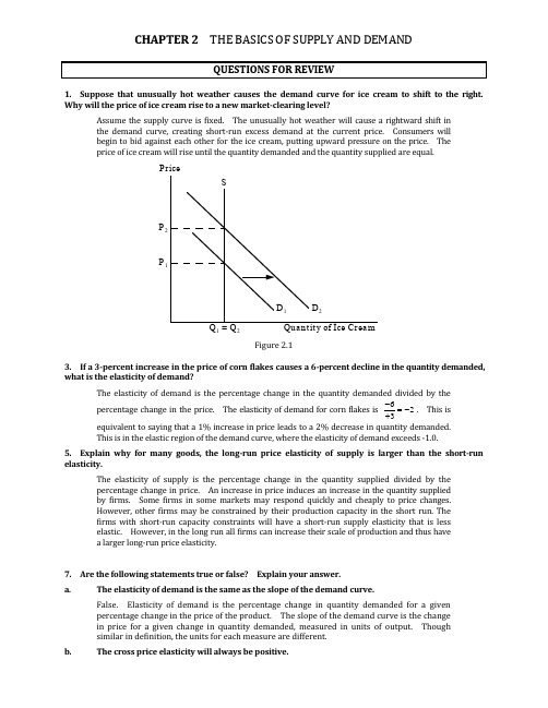
The elasticity of supply is the percentage change in the quantity supplied divided by the percentage change in price. An increase in price induces an increase in the quantity supplied by firms. Some firms in some markets may respond quickly and cheaply to price changes.However, other firms may be constrained by their production capacity in the short run. The firms with short-run capacity constraints will have a short-run supply elasticity that is less elastic. However, in the long run all firms can increase their scale of production and thus havea larger long-run price elasticity.7. Are the following statements true or false? Explain your answer.a. The elasticity of demand is the same as the slope of the demand curve.False. Elasticity of demand is the percentage change in quantity demanded for a given percentage change in the price of the product. The slope of the demand curve is the change in price for a given change in quantity demanded, measured in units of output. Though similar in definition, the units for each measure are different.b. The cross price elasticity will always be positive.False. The cross price elasticity measures the percentage change in the quantity demanded of one product for a given percentage change in the price of another product. This elasticity will be positive for substitutes (an increase in the price of hot dogs is likely to cause an increase in the quantity demanded of hamburgers) and negative for complements (an increase in the price of hot dogs is likely to cause a decrease in the quantity demanded of hot dog buns).c. The supply of apartments is more inelastic in the short run than the long run.True. In the short run it is difficult to change the supply of apartments in response to a change in price. Increasing the supply requires constructing new apartment buildings, which can take a year or more. Since apartments are a durable good, in the long run a change in price will induce suppliers to create more apartments (if price increases) or delay construction (if price decreases).9. The city council of a small college town decides to regulate rents in order to reduce student living expenses. Suppose the average annual market-clearing rent for a two-bedroom apartment had been $700 per month, and rents are expected to increase to $900 within a year. The city council limits rents to their current $700 per month level. a. Draw a supply and demand graph to illustrate what will happen to the rental price of an apartment after the imposition of rent controls.The rental price will stay at the old equilibrium level of $700 per month. The expected increase to $900 per month may have been caused by an increase in demand. Given this is true, the price of $700 will be below the new equilibrium and there will be a shortage of apartments.b. Do you think this policy will benefit all students? Why or why not.It will benefit those students who get an apartment, though these students may also find that the costs of searching for an apartment are higher given the shortage of apartments. Those students who do not get an apartment may face higher costs as a result of having to live outside of the college town. Their rent may be higher and the transportation costs will be higher.11. Suppose the demand curve for a product is given by Q=10-2P+P s , where P is the price of the product and P s is the price of a substitute good. The price of the substitute good is $2.00.a. Suppose P=$1.00. What is the price elasticity of demand? What is the cross-price elasticity of demand?First you need to find the quantity demanded at the price of $1.00. Q=10-2(1)+2=10. Priceelasticity of demand = P Q ∆Q ∆P =110(-2)=-210=-0.2. Cross-price elasticity of demand =P s Q ∆Q ∆P s =210(1)=0.2. b. Suppose the price of the good, P, goes to $2.00. Now what is the price elasticity of demand? What is the cross-price elasticity of demand?First you need to find the quantity demanded at the price of $2.00. Q=10-2(2)+2=8.Price elasticity of demand = P Q ∆Q ∆P =28(-2)=-48=-0.5. Cross-price elasticity of demand = P s Q ∆Q ∆P s =28(1)=0.25. 13. Suppose the demand for natural gas is perfectly inelastic. What would be the effect, if any, of natural gas price controls?If the demand for natural gas is perfectly inelastic, then the demand curve is vertical.Consumers will demand a certain quantity and will pay any price for this quantity. In this case,a price control will have no effect on the quantity demanded.1. Suppose the demand curve for a product is given by Q=300-2P+4I, where I is average income measured in thousands of dollars. The supply curve is Q=3P-50.a. If I=25, find the market clearing price and quantity for the product.Given I=25, the demand curve becomes Q=300-2P+4*25, or Q=400-2P. Setting demand equalto supply we can solve for P and then Q:400-2P=3P-50P=90Q=220.b. If I=50, find the market clearing price and quantity for the product.Given I=50, the demand curve becomes Q=300-2P+4*50, or Q=500-2P. Setting demand equalto supply we can solve for P and then Q:500-2P=3P-50P=110Q=280.c. Draw a graph to illustrate your answers.Equilibrium price and quantity are found at the intersection of the demand and supply curves.When the income level increases in part b, the demand curve will shift up and to the right. Theintersection of the new demand curve and the supply curve is the new equilibrium point.3. Refer to Example 2.5 on the market for wheat. At the end of 1998, both Brazil and Indonesia opened their wheat markets to U.S. farmers. Suppose that these new markets add 200 million bushels to U.S. wheat demand. What will be the free market price of wheat and what quantity will be produced and sold by U.S. farmers in this case?The following equations describe the market for wheat in 1998:Q S = 1944 + 207PandQ D = 3244 - 283P.If Brazil and Indonesia add an additional 200 million bushels of wheat to U.S. wheat demand,the new demand curve would be equal to Q D + 200, orQ D = (3244 - 283P) + 200 = 3444 - 283P.Equating supply and the new demand, we may determine the new equilibrium price,1944 + 207P = 3444 - 283P, or490P = 1500, or P* = $3.06122 per bushel.To find the equilibrium quantity, substitute the price into either the supply or demand equation,e.g.,Q S = 1944 + (207)(3.06122) = 2,577.67andQ D = 3444 - (283)(3.06122) = 2,577.677. In 1998, Americans smoked 470 billion cigarettes, or 23.5 billion packs of cigarettes. The average retail price was $2 per pack. Statistical studies have shown that the price elasticity of demand is -0.4, and the price elasticity of supply is 0.5. Using this information, derive linear demand and supply curves for the cigarette market.Let the demand curve be of the general form Q=a-bP and the supply curve be of the general form Q=c + dP, where a, b, c, and d are the constants that you have to find from the information given above. To begin, recall the formula for the price elasticity of demandE P D =P Q ∆Q ∆P. You are given information about the value of the elasticity, P, and Q, which means that you can solve for the slope, which is b in the above formula for the demand curve.-0.4=223.5∆Q∆P ∆Q ∆P=-0.423.52⎛ ⎝ ⎫ ⎭ =-4.7=-b . To find the constant a, substitute for Q, P, and b into the above formula so that 23.5=a-4.7*2 and a=32.9. The equation for demand is therefore Q=32.9-4.7P. To find the supply curve, recall the formula for the elasticity of supply and follow the same method as above:E P S =P Q ∆Q∆P0.5=223.5∆Q ∆P∆Q ∆P =0.523.52⎛ ⎝ ⎫ ⎭ =5.875=d . To find the constant c, substitute for Q, P, and d into the above formula so that 23.5=c+5.875*2 and c=11.75. The equation for supply is therefore Q=11.75+5.875P.9. Example 2.9 analyzes the world oil market. Using the data given in that example:a. Show that the short-run demand and competitive supply curves are indeed given byD = 24.08 - 0.06PS C = 11.74 + 0.07P .First, considering non-OPEC supply:S c = Q * = 13.With E S = 0.10 and P * = $18, E S = d (P */Q *) implies d = 0.07.Substituting for d , S c , and P in the supply equation, c = 11.74 and S c = 11.74 + 0.07P .Similarly, since Q D = 23, E D = -b (P */Q *) = -0.05, and b = 0.06. Substituting for b , Q D = 23, and P = 18 in the demand equation gives 23 = a - 0.06(18), so that a = 24.08.Hence Q D = 24.08 - 0.06P .b. Show that the long-run demand and competitive supply curves are indeed given byD = 32.18 - 0.51PS C = 7.78 + 0.29P .As above, E S = 0.4 and E D = -0.4: E S = d (P */Q *) and E D = -b(P*/Q*), implying 0.4 = d (18/13) and -0.4 = -b (18/23). So d = 0.29 and b = 0.51.Next solve for c and a :S c = c + dP and Q D = a - bP , implying 13 = c + (0.29)(18) and 23 = a - (0.51)(18).So c = 7.78 and a = 32.18.c. In 2002, Saudi Arabia accounted for 3 billion barrels per year of OPEC’s production. Suppose that war or revolution caused Saudi Arabia to stop producing oil. Use the model above tocalculate what would happen to the price of oil in the short run and the long run if OPEC’s production were to drop by 3 billion barrels per year.With OPEC’s supply reduced from 10 bb/yr to 7 bb/yr, add this lower supply of 7 bb/yr to the short -run and long-run supply equations:S c ' = 7 + S c = 11.74 + 7 + 0.07P = 18.74 + 0.07P and S " = 7 + S c = 14.78 + 0.29P .These are equated with short-run and long-run demand, so that:18.74 + 0.07P = 24.08 - 0.06P ,implying that P = $41.08 in the short run; and14.78 + 0.29P = 32.18 - 0.51P ,implying that P = $21.75 in the long run.10.Refer to Example 2.10, which analyzes the effects of price controls on natural gas. a. Using the data in the example, show that the following supply and demand curves did indeed describe the market in 1975:Supply: Q = 14 + 2P G + 0.25P ODemand: Q = -5P G + 3.75P Owhere P G and P O are the prices of natural gas and oil, respectively. Also, verify that if the price of oil is $8.00, these curves imply a free market price of $2.00 for natural gas.To solve this problem, we apply the analysis of Section 2.6 to the definition of cross-price elasticity of demand given in Section 2.4. For example, the cross-price-elasticity of demand for natural gas with respect to the price of oil is:E GO =∆Q G ∆P O ⎛ ⎝ ⎫ ⎭ ⎪ P O Q G ⎛ ⎝ ⎫ ⎭⎪ . ∆Q G ∆P O ⎛ ⎝ ⎫ ⎭⎪ is the change in the quantity of natural gas demanded, because of a small change in the price of oil. For linear demand equations, ∆Q G ∆P O ⎛ ⎝ ⎫ ⎭⎪ is constant. If we represent demand as: Q G = a - bP G + eP O(notice that income is held constant), then ∆Q G ∆P O ⎛ ⎝ ⎫ ⎭⎪ = e . Substituting this into the cross-price elasticity, E PO =e P O *Q G *⎛ ⎝ ⎫ ⎭⎪ , where P O * and Q G * are the equilibrium price and quantity. We know that P O * = $8 and Q G* = 20 trillion cubic feet (Tcf). Solving for e , 1.5=e 820⎛ ⎝ ⎫ ⎭, or e = 3.75. Similarly, if the general form of the supply equation is represented as:Q G = c + dP G + gP O ,the cross-price elasticity of supply is g P O *Q G *⎛ ⎝ ⎫ ⎭⎪ , which we know to be 0.1. Solving for g , 0.1=g 820⎛ ⎝ ⎫ ⎭, or g = 0.25.The values for d and b may be found with equations 2.5a and 2.5b in Section 2.6. We know that E S = 0.2, P* = 2, and Q* = 20. Therefore,0.2=d220⎛⎝⎫⎭ , or d = 2.Also, E D = -0.5, so-0.5=b 2 20⎛ ⎝ ⎫⎭ , or b = -5.By substituting these values for d, g, b, and e into our linear supply and demand equations, wemay solve for c and a:20 = c + (2)(2) + (0.25)(8), or c = 14,and20 = a - (5)(2) + (3.75)(8), or a = 0.If the price of oil is $8.00, these curves imply a free market price of $2.00 for natural gas.Substitute the price of oil in the supply and demand curves to verify these equations. Then setthe curves equal to each other and solve for the price of gas.14 + 2P G + (0.25)(8) = -5P G + (3.75)(8)7P G= 14P G= $2.00.b. Suppose the regulated price of gas in 1975 had been $1.50 per thousand cubic feet, instead of$1.00. How much excess demand would there have been?With a regulated price of $1.50 for natural gas and a price of oil equal to $8.00 per barrel,Demand: Q D = (-5)(1.50) + (3.75)(8) = 22.5, andSupply: Q S = 14 + (2)(1.5) + (0.25)(8) = 19.With a supply of 19 Tcf and a demand of 22.5 Tcf, there would be an excess demand of 3.5 Tcf.c. Suppose that the market for natural gas had not been regulated. If the price of oil had increasedfrom $8 to $16, what would have happened to the free market price of natural gas?If the price of natural gas had not been regulated and the price of oil had increased from $8 to$16, thenDemand: Q D = -5P G + (3.75)(16) = 60 - 5P G, andSupply: Q S= 14 + 2P G+ (0.25)(16) = 18 + 2P G.Equating supply and demand and solving for the equilibrium price,18 + 2P G = 60 - 5P G, or P G = $6.The price of natural gas would have tripled from $2 to $6.。

计算题讲解1.已知某一时期内某商品的需求函数为Q d=50-5P,供给函数为Q s=-20+5P。

（1）求均衡价格P e和均衡数量Q e。

（2）假设供给函数不变，由于消费者收入水平提高，使需求函数变为Q d=60-5P, 求出相应的均衡价格P e和均衡数量Q e。

解：（1）因为Q d＝Q S时达到供求均衡即50–5P＝–20+5P 得均衡价格Pe=7均衡数量Qe=50–5×7=15（2）因为Q d＝Q S时达到供求均衡即60–5P＝–20+5P 得均衡价格Pe=8均衡数量Qe=60–5×8=202．已知某商品的需求函数为Q d=500-100P。

该商品的需求表如下：价格（元） 1 2 3 4 5需求量400 300 200 100 0（1）求出价格2元和4元之间的需求的价格弧弹性。

（2）根据需求函数，求出P＝2元时的需求的价格点弹性。

解.（1）求价格2元到4元之间的需求的价格弧弹性e d=–(∆Q/∆P)×[（P1+P2）/2]÷[（Q1+Q2）/2]=–[(100-300)÷(4-2)]×[（2+4）/2]÷[（300+100）/2]=–[(-200)÷2]×[3÷200]=1.5（2）求P=2元时需求的价格点弹性e d=–(dQ/dP)×(P/Q)=–(-100)×(2÷300)=2/33.已知完全竞争市场下某厂商的短期总成本函数为TC(Q)=4Q3+5Q2+6Q+200，求：（1）该厂商的短期可变成本函数？（2）该厂商的短期固定成本是多少？（3）该厂商的短期边际成本函数？（4）该厂商的短期平均成本函数？（5）该厂商的短期平均可变成本函数？解：（1）该厂商的短期可变成本函数为TC(Q)=4 Q3+5Q2+6Q（2）该厂商的短期固定成本是200（3）该厂商的短期边际成本函数是其总成本函数的一阶导数，即MC(Q)=12Q2+10Q+6（4）该厂商的短期平均成本函数AC(Q)=4Q2+5Q+6+200/Q（5）该厂商的短期平均可变成本函数AVC(Q)=4Q2+5Q+64、假设某消费者的均衡如右图所示。

微观经济学计算题1.已知某商品的需求方程和供给方程分别为Q d =14-3P, Q s =2+6P 。

求：该商品的均衡价格和均衡产销量，以及均衡时的需求价格弹性和供给价格弹性。

均衡时，供给量等于需求量，Q d =Q s ，也就是14－3P=2+6P ，2.已知某商品的需求方程和供给方程分别为Q d =30-P ，Q s =10+3P ，试求：（1）该商品的均衡价格；（2）均衡时的需求价格弹性和供给弹性。

3.假设A 公司和B 公司的产品的需求曲线分别为Q A =200-0.2P A ，Q B =400-0.25P B ，这两家公司现在的销售量分别为100和250。

求这两家公司当前的需求价格弹性。

4.假定在某市场上A 、B 两厂商是生产同种有差异的产品的竞争者；该市场对A 厂商的需求曲线为P A ＝200－Q A ，对B 厂商的需求曲线为P B ＝300－0.5Q B ；两厂商目前的销售量分别为Q A ＝50，Q B ＝100。

求：A 、B 两厂商的需求的价格弹性各是多少？关于A 厂商：5.已知某垄断厂商利用一个工厂生产一种产品，其产品在两个分割的市场上出售，他的成本函数为Q Q TC 402+=，两个市场的需求函数分别为111.012P Q -=，224.020P Q -=。

求：(1) 当该厂商实行三级价格歧视时，他追求利润最大化前提下的两个市场各自的销售量、价格以及厂商的总利润。

(2) 当该厂商在两个市场实行统一的价格时，他追求利润最大化前提下的销售量、价格以及厂商的总利润。

6.某垄断厂商所生产的产品在两个分割的市场出售，产品的成本函数为TC=Q2+10Q，两个市场的需求函数分别为Q1=32-0.4P1，Q2=18-0.1P2，求：(1) 当该厂商实行三级价格歧视时，他追求利润最大化前提下的两个市场各自的销售量、价格以及厂商的总利润。

(2) 当该厂商在两个市场实行统一的价格时，他追求利润最大化前提下的销售量、价格以及厂商的总利润。

《微观经济学》计算题参考答案微观经济学计算题参考答案第2章10、（1）13，21；（2）15，25；（3）14，18（书后答案须更正）。

（1）根据需求函数和供给函数联⽴⽅程组：（2）同（1），联⽴⽅程组：（3）同（1），联⽴⽅程组：70-3P=-5+2P P=15Q d ＝70-3×15＝25 Q s ＝-5+2×15＝2560-3P=-5+2P P=13Q d ＝60-3×13＝21 Q s ＝-5+2×13＝21第3章5、（1）-5/3；（2）-1。

（1）P 1＝4时，Q 1＝200-25×4＝100； P 2＝6时，Q 2＝200-25×6＝50；12d 1246501005010522E 10050642150322P P Q Q Q P++?--==?=?=-++?-（2）代数法：当P ＝4时，Q ＝100；根据点弹性公式有d 4E (25)1100dQPdP Q==-=-⼏何法（参看第49页图3.2）：当P ＝4时，Q ＝100，所以OP 1=4。

令Q ＝0，则0＝200-25P ，P ＝8，所以OP 0＝8。

由于OP 1=4，P 0P 1＝OP 0-OP 1＝8-4＝4。

根据⼏何法公式：60-3P=-10+2P P=14Q d ＝60-3×14＝18 Q s ＝-10+2×14＝181d 014E 14O P P P =-=-=-6、（1）4/3；（2）2。

（原题⽬中的需求改为供给）（1）P 1＝8时，Q 1＝-100+25×8＝100； P 2＝24时，Q 2＝-100-25×24＝500；12s 1282450010040032422E 10050024816600322P P Q Q Q P++?-==?=?=++?-（2）代数法：当P ＝8时，Q ＝100；根据点弹性公式有s 8E 252P dP Q===⼏何法（参看第54页图3.6）：当P ＝8时，Q ＝100，所以OP 1=8。