纳什均衡哈佛第六讲
- 格式:pdf
- 大小:104.02 KB
- 文档页数:12


举个简单的例子来说明博奕论是什么?你在一个屋子里,屋里有很多人。
这时候,屋里突然失火,火势很大,无法扑灭。
此时你的目的就是逃生。
你的面前有两个门,左门和右门,你必须在它们之间选择。
但问题是,其他人也要争抢这两个门出逃。
如果你选择的门是很多人选择的,那么你将因人多拥挤、冲不出去而烧死;相反,如果你选择的是较少人选择的,那么你将逃生。
这里我们不考虑道德因素,你将如何选择?——这就是博弈论!你的选择必须考虑其他人的选择,而其他人的选择也考虑你的选择。
你的结果(博弈论称之为支付pay off),不仅取决于你的行动选择(博弈论称之为策略选择),同时取决于他人的策略选择。
你和这群人构成一个博弈(game)。
博弈论对人的基本假定是:人是理性的(rational)。
所谓理性的人是指他在具体策略选择时的目的是使自己的利益最大化,博弈论研究的是理性的人之间如何进行策略选择的。
中国人对博弈论有天生的了解。
正如中国人常说的“事事洞明皆学问,人情练达即文章”,即是说人与人之间的关系、社会交往均是学问。
而中国很多“做人”的道理,道出了如何在人与人的博弈中获取成功。
罗贯中的《三国演义》在今天看来就是一部博弈论教材!无论是兵书如《孙子兵法》、《三十六计》,还是现代流行的所谓“厚黑学”,都是关于如何赢得与人交往的胜利的,或者说如何获取成功的.博奕论中流传最广的是一个叫做“囚徒困境”的故事。
说的是两个囚犯的故事。
这两个囚徒一起做坏事,结果被警察发现抓了起来,分别关在两个独立的不能互通信息的牢房里进行审讯。
在这种情形下,两个囚犯都可以做出自己的选择:或者供出他的同伙(即与警察合作,从而背叛他的同伙),或者保持沉默(也就是与他的同伙合作,而不是与警察合作)。
如果他们中的一个人背叛,即告发他的同伙,那么他就可以被无罪释放。
而他的同伙就会被判10年。
如果双方都与警方合作共同招认,则各被判5年。
如果双方均不承认有罪,因警察找不到其他证据来证明他们以前的违法证据,则各判3个月。


博弈论-纳什均衡(非合作博弈均衡)完全理性:理性指一种行为方式,它适合实现指定目标,而且在给定条件和约束的限度之内。
在不同的学科领域,理性所涵盖的内容存在着差异完全理性的内涵具有完全理性的行为人是个无所不知的超人,他具有纵向和横向方面完备的知识。
在纵向方面,他可以预测未来;在横向方面,他通晓资源、交易伙伴和环境等情况。
具体而言,行为人的完全理性包括以下隐含内容。
(1)不存在不确定性,即使存在不确定性,也可以预知不确定性的概率分布。
也就是说,对于具有完全理性的行为人来说,一切信息都是确定的。
(2)行为人具有可以确定的效用函数(消费者的效用函数和厂商的利润函数可以统称为效用函数),同时行为人具有同质性以及一致性的偏好体系。
(3)选择结果具有描述不变性、程序不变性和前后关系独立性。
描述不变性要求行为人选择的先后顺序不应依赖于所描述或显示的选项,也就是说如果行为人经过再三思考,将两种描述视为同一问题的同义表达,那么它们必定导致相同的选择——即这种思考不存在异处;程序不变性要求不同方式的等价学说揭露相同的偏好次序;前后关系独立性指一项选择与其他替代方案互为独立的原则,它要求在给定Z而不提供有关X或Y 的新的信息的情况下,X 与Y的优先权顺序不应该依赖于Z是否有效。
(4)行为人具备完备的计算和推理能力,可以像计算机一样在数秒内从事无穷尽的计算步骤,同时也不存在感性因素对选择的干扰。
(5)选择意味着在各种方案或选择集中进行比较和挑选,因此完全理性的行为人可以设计出所有的被选方案,以及各项方案所产生的全部后果。
(6)一个确定的报酬函数,即行为人可以确定地赋予每项行动结果一个具体的量化价值或效用。
(7)确定性的结果,也就是行为人町以实现效用最大化或最优目标(消费者效用最大化和企业利润最大化)。
在上述条件下,建立在完全理性假设的基础上的主流经济学的方法论,即行为人的选择或决策意味着在资源约束的条件下实现效用最大化或利润最大化。


纳什均衡的定义:在博弈G=﹛S1,…,Sn:u1,…,un﹜中,如果由各个博弈方的各一个策略组成的某个策略组合(s1*,…,sn*)中,任一博弈方i的策略si*,都是对其余博弈方策略的组合(s1*,…s*i-1,s*i+1,…,sn*)的最佳对策,也即ui(s1*,…s*i-1,si*,s*i+1,…,sn*)≥ui(s1*,…s*i-1,sij*,s*i+1,…,sn*)对任意sij∈Si都成立,则称(s1*,…,sn*)为G的一个纳什均衡。
纳什均衡是一种策略组合, 在顺序博弈中这个均衡是在博弈者连续的动作与反应中达成, 只有最优策略才可以达成纳什均衡.
例子:囚徒困境。
一个事件中不止一个纳什均衡。
完全信息动态博弈,子博弈精炼纳什均衡。
不可置信的威胁策略剔除.
不完全信息动态博弈,贝叶斯纳什均衡。
在不完全信息静态博弈中,参与人同时行动,没有机会观察到别人的选择。
给定其他参与人的战略选择,每个参与人的最优战略依赖于自己的类型。
由于每个参与人仅知道其他参与人有关类型的分布概率,而不知道其真实类型,因而,他不可能知道其他参与人实际上会选择什么战略。
但是,他能够正确地预测到其他参与人的选择与其各自的有关类型之间的关系。
在给定自己的类型,以及给定其他参与人的类型与战略选择之间关系的条件下,使得自己的期望效用最大化。
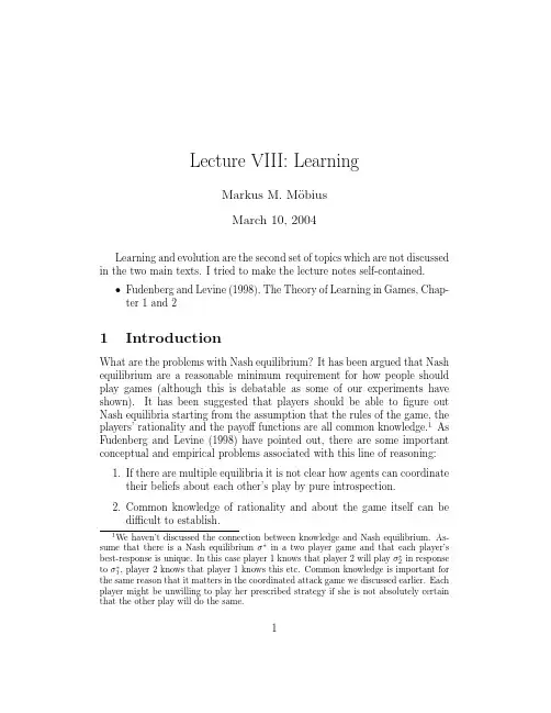
Lecture VIII:LearningMarkus M.M¨o biusMarch10,2004Learning and evolution are the second set of topics which are not discussed in the two main texts.I tried to make the lecture notes self-contained.•Fudenberg and Levine(1998),The Theory of Learning in Games,Chap-ter1and21IntroductionWhat are the problems with Nash equilibrium?It has been argued that Nash equilibrium are a reasonable minimum requirement for how people should play games(although this is debatable as some of our experiments have shown).It has been suggested that players should be able tofigure out Nash equilibria starting from the assumption that the rules of the game,the players’rationality and the payofffunctions are all common knowledge.1As Fudenberg and Levine(1998)have pointed out,there are some important conceptual and empirical problems associated with this line of reasoning:1.If there are multiple equilibria it is not clear how agents can coordinatetheir beliefs about each other’s play by pure introspection.mon knowledge of rationality and about the game itself can bedifficult to establish.1We haven’t discussed the connection between knowledge and Nash equilibrium.As-sume that there is a Nash equilibriumσ∗in a two player game and that each player’s best-response is unique.In this case player1knows that player2will playσ∗2in response toσ∗1,player2knows that player1knows this mon knowledge is important for the same reason that it matters in the coordinated attack game we discussed earlier.Each player might be unwilling to play her prescribed strategy if she is not absolutely certain that the other play will do the same.13.Equilibrium theory does a poor job explaining play in early rounds ofmost experiments,although it does much better in later rounds.This shift from non-equilibrium to equilibrium play is difficult to reconcile with a purely introspective theory.1.1Learning or Evolution?There are two main ways to model the processes according to which players change their strategies they are using to play a game.A learning model is any model that specifies the learning rules used by individual players and examines their interaction when the game(or games)is played repeatedly. These types of models will be the subject of today’s lecture.Learning models quickly become very complex when there are many play-ers involved.Evolutionary models do not specifically model the learning process at the individual level.The basic assumption there is that some un-specified process at the individual level leads the population as a whole to adopt strategies that yield improved payoffs.These type of models will the subject of the next few lectures.1.2Population Size and MatchingThe natural starting point for any learning(or evolutionary)model is the case offixed players.Typically,we will only look at2by2games which are played repeatedly between these twofixed players.Each player faces the task of inferring future play from the past behavior of agents.There is a serious drawback from working withfixed agents.Due to the repeated interaction in every game players might have an incentive to influence the future play of their opponent.For example,in most learning models players will defect in a Prisoner’s dilemma because cooperation is strictly dominated for any beliefs I might hold about my opponent.However, if I interact frequently with the same opponent,I might try to cooperate in order to’teach’the opponent that I am a cooperator.We will see in a future lecture that such behavior can be in deed a Nash equilibrium in a repeated game.There are several ways in which repeated play considerations can be as-sumed away.1.We can imagine that players are locked into their actions for quite2a while(they invest infrequently,can’t build a new factory overnightetc.)and that their discount factors(the factor by which they weight the future)is small compared that lock-in length.It them makes sense to treat agents as approximately myopic when making their decisions.2.An alternative is to dispense with thefixed player assumption,andinstead assume that agents are drawn from a large population and are randomly matched against each other to play games.In this case,it is very unlikely that I encounter a recent opponent in a round in the near future.This breaks the strategic links between the rounds and allows us to treat agents as approximately myopic again(i.e.they maximize their short-term payoffs).2Cournot AdjustmentIn the Cournot adjustment model twofixed players move sequentially and choose a best response to the play of their opponent in the last period.The model was originally developed to explain learning in the Cournotmodel.Firms start from some initial output combination(q01,q02).In thefirst round bothfirms adapt their output to be the best response to q02.Theytherefore play(BR1(q02),BR2(q01)).This process is repeated and it can be easily seen that in the case of linear demand and constant marginal costs the process converges to the unique Nash equilibrium.If there are several Nash equilibria the initial conditions will determine which equilibrium is selected.2.1Problem with Cournot LearningThere are two main problems:•Firms are pretty dim-witted.They adjust their strategies today as if they expectfirms to play the same strategy as yesterday.•In each period play can actually change quite a lot.Intelligentfirms should anticipate their opponents play in the future and react accord-ingly.Intuitively,this should speed up the adjustment process.3Cournot adjustment can be made more realistic by assuming thatfirms are’locked in’for some time and that they move alternately.Firms1moves in period1,3,5,...andfirm2moves in periods2,4,6,..Starting from someinitial play(q01,q02),firms will play(q11,q02)in round1and(q11,q22)in round2.Clearly,the Cournot dynamics with alternate moves has the same long-run behavior as the Cournot dynamics with simultaneous moves.Cournot adjustment will be approximately optimal forfirms if the lock-in period is large compared to the discount rate offirms.The less locked-in firms are the smaller the discount rate(the discount rate is the weight on next period’s profits).Of course,the problem with the lock-in interpretation is the fact that it is not really a model of learning anymore.Learning is irrelevant becausefirms choose their optimal action in each period.3Fictitious PlayIn the process offictitious play players assume that their opponents strategies are drawn from some stationary but unknown distribution.As in the Cournot adjustment model we restrict attention to afixed two-player setting.We also assume that the strategy sets of both players arefinite.4Infictitious play players choose the best response to their assessment of their opponent’s strategy.Each player has some exogenously given weightingfunctionκ0i :S−i→ +.After each period the weights are updated by adding1to each opponent strategy each time is has been played:κt i (s−i)=κt−1i(s−i)if s−i=s t−1−iκt−1i(s−i)+1if s−i=s t−1−iPlayer i assigns probabilityγti(s−i)to strategy profile s−i:γt i (s−i)=κti(s−i)˜s−i∈S−iκti(˜s−i)The player then chooses a pure strategy which is a best response to his assessment of other players’strategy profiles.Note that there is not neces-sarily a unique best-response to every assessment-hencefictitious play is not always unique.We also define the empirical distribution d ti (s i)of each player’s strategiesasd t i (s i)=t˜t=0I˜t(s i)tThe indicator function is set to1if the strategy has been played in period˜tand0otherwise.Note,that as t→∞the empirical distribution d tj of playerj’s strategies approximate the weighting functionκti (since in a two playergame we have j=−i).Remark1The updating of the weighting function looks intuitive but also somewhat arbitrary.It can be made more rigorous in the following way. Assume,that there are n strategy profiles in S−i and that each profile is played by player i’s opponents’with probability p(s−i).Agent i has a prior belief according to which these probabilities are distributed.This prior is a Dirichlet distribution whose parameters depend on the weighting function. After each round agents update their prior:it can be shown that the posterior belief is again Dirichlet and the parameters of the posterior depend now on the updated weighting function.3.1Asymptotic BehaviorWillfictitious play converge to a Nash equilibrium?The next proposition gives a partial answer.5Proposition1If s is a strict Nash equilibrium,and s is played at date t in the process offictitious play,s is played at all subsequent dates.That is,strict Nash equilibria are absorbing for the process offictitious play.Furthermore, any pure-strategy steady state offictitious play must be a Nash equilibrium. Proof:Assume that s=(s i,s j)is played at time t.This implies that s i isa best-response to player i’s assessment at time t.But his next periodassessment will put higher relative weight on strategy s j.Because s i isa BR to s j and the old assessment it will be also a best-response to theupdated assessment.Conversely,iffictitious play gets stuck in some pure steady state then players’assessment converge to the empirical distribution.If the steady state is not Nash players would eventually deviate.A corollary of the above result is thatfictitious play cannot converge to a pure steady state in a game which has only mixed Nash equilibria such as matchingpennies.6distribution over each player’s strategies are converging to12,12-this isprecisely the unique mixed Nash equilibrium.This observation leads to a general result.Proposition2Underfictitious play,if the empirical distributions over each player’s choices converge,the strategy profile corresponding to the product of these distributions is a Nash equilibrium.Proof:Assume that there is a profitable deviation.Then in the limit at least one player should deviate-but this contradicts the assumption that strategies converge.These results don’t tell us whenfictitious play converges.The next the-orem does precisely that.Theorem1Underfictitious play the empirical distributions converge if the stage has generic payoffs and is22,or zero sum,or is solvable by iterated strict dominance.We won’t prove this theorem in this lecture.However,it is intuitively clear whyfictitious play observes IDSDS.A strictly dominated strategy can never be a best response.Therefore,in the limitfictitious play should put zero relative weight on it.But then all strategies deleted in the second step can never be best responses and should have zero weight as well etc.3.2Non-Convergence is PossibleFictitious play does not have to converge at all.An example for that is due to Shapley.7(M,R),(M,L),(D,L),(D,M),(T,M).One can show that the number of time each profile is played increases at a fast enough rate such that the play never converges.Also note,that the diagonal entries are never played.3.3Pathological ConvergenceConvergence in the empirical distribution of strategy choices can be mis-leading even though the process converges to a Nash equilibrium.Take the following game:8riod the weights are2,√2,and both play B;the outcome is the alternatingsequence(B,B),(A,A),(B,B),and so on.The empirical frequencies of each player’s choices converge to1/2,1/2,which is the Nash equilibrium.The realized play is always on the diagonal,however,and both players receive payoff0each period.Another way of putting this is that the empirical joint distribution on pairs of actions does not equal the product of the two marginal distributions,so the empirical joint distribution corresponds to correlated as opposed to independent play.This type of correlation is very appealing.In particular,agents don’t seem to be smart enough to recognize cycles which they could exploit.Hence the attractive property of convergence to a Nash equilibrium can be misleading if the equilibrium is mixed.9。

纳什均衡,又称为非合作博弈均衡,是博弈论的一个重要术语,以约翰·纳什命名。
在一个博弈过程中,无论对方的策略选择如何,当事人一方都会选择某个确定的策略,则该策略被称作支配性策略。
如果两个博弈的当事人的策略组合分别构成各自的支配性策略,那么这个组合就被定义为纳什均衡。
一个策略组合被称为纳什均衡,当每个博弈者的均衡策略都是为了达到自己期望收益的最大值,与此同时,其他所有博弈者也遵循这样的策略。
[编辑]纳什均衡的得来关于纳什均衡的普遍意义和存在性定理的证明等奠定非合作博弈理论发展基础的重要成果,是约翰·纳什在普林斯顿大学攻读博士学位时完成的。
实际上,博弈论的研究起始于1944年冯·诺依曼(Von Neumann)和奥斯卡·摩根斯坦(Oscar Morgenstern)合著的《博弈论和经济行为》。
然而却是纳什首先用严密的数学语言和简明的文字准确地定义了纳什均衡这个概念,并在包含“混合策略(mixed strategies)”的情况下,证明了纳什均衡在n人有限博弈中的普遍存在性,从而开创了与诺依曼和摩根斯坦框架路线均完全不同的“非合作博弈(Non-cooperative Game)”理论,进而对“合作博弈(Cooperative Game)”和“非合作博弈”做了明确的区分和定义。
阿尔伯特·塔克(Albert tucker)教授评价其论文,“这是对博弈理论的高度原创性和重要的贡献。
它发展了本身很有意义的n人有限非合作博弈的概念和性质。
并且它很可能开拓出许多在两人零和问题以外的,至今尚未涉及的问题。
在概念和方法两方面,该论文都是作者的独立创造。
”[编辑]在一个博弈过程中,无论对方的策略选择如何,当事人一方都会选择某个确定的策略,则该策略被称作支配性策略。
如果两个博弈的当事人的策略组合分别构成各自的支配性策略,那么这个组合就被定义为纳什均衡。
纳什均衡又称为非合作博弈均衡,是博弈论的一个重要术语,它是以美国数学家、日后成为电影《美丽心灵》主人公的纳什的名字命名的。
实例说明什么是纳什均衡电影《美丽心灵》的主人公原型约翰·纳什车祸于2015年5月23日去世。
你也许听说过他是厉害的数学家、1994年诺贝尔经济学奖得主、博弈论之父……但是,他的最大贡献是“纳什均衡”。
纳什均衡到底是个什么看看纳什均衡的经济学定义:所谓纳什均衡,指的是参与人的这样一种策略组合,在该策略组合上,任何参与人单独改变策略都不会得到好处。
换句话说,如果在一个策略组合上,当所有其他人都不改变策略时,没有人会改变自己的策略,则该策略组合就是一个纳什均衡。
是不是看完几乎没什么概念?我们先用个常见的现象试图解释下,例如价格战。
生产同一样产品的若干厂家会形成一个稳定的状态,在这个状态下各家所卖的产品价格保持基本一致,在这种情况下各方就形成了一个“纳什均衡”。
若其中一方打破默契,开始大幅降价,以求薄利多销,获取更大利润,那么其他家便会很快跟进,互相压价。
刚开始降价的一方短期内可能会增加销量和利润,但最终的结果是两败俱伤。
下面小编将给大家举几个经典的例子,以便大家更深刻地理解约翰·纳什这位奇才留给我们的精神遗产。
囚徒困境假设有两个小偷A和B联合犯事、私入民宅被警察抓住。
警方将两人分别置于不同的两个房间内进行审讯,对每一个犯罪嫌疑人,警方给出的政策是:如果一个犯罪嫌疑人坦白了罪行,交出了赃物,于是证据确凿,两人都被判有罪。
如果另一个犯罪嫌疑人也作了坦白,则两人各被判刑8年。
如果另一个犯罪嫌人没有坦白而是抵赖,则以妨碍公务罪(因已有证据表明其有罪)再加刑2年,而坦白者有功被减刑8年,立即释放。
如果两人都抵赖,则警方因证据不足不能判两人的偷窃罪,但可以私入民宅的罪名将两人各判入狱1年。
关于案例,显然最好的策略是双方都抵赖,结果是大家都只被判1年。
但是由于两人处于隔离的情况,首先应该是从心理学的角度来看,当事双方都会怀疑对方会出卖自己以求自保、其次才是亚当·斯密的理论,假设每个人都是“理性的经济人”,都会从利己的目的出发进行选择。
Lecture VI:Existence of Nash equilibriumMarkus M.M¨o biusFebruary26,2008•Osborne,chapter4•Gibbons,sections1.3.B1Nash’s Existence TheoremWhen we introduced the notion of Nash equilibrium the idea was to come up with a solution concept which is stronger than IDSDS.Today we show that NE is not too strong in the sense that it guarantees the existence of at least one mixed Nash equilibrium in most games(for sure in allfinite games). This is reassuring because it tells that there is at least one way to play most games.1Let’s start by stating the main theorem we will prove:Theorem1(Nash Existence)Everyfinite strategic-form game has a mixed-strategy Nash equilibrium.Many game theorists therefore regard the set of NE for this reason as the lower bound for the set of reasonably solution concept.A lot of research has gone into refining the notion of NE in order to retain the existence result but get more precise predictions in games with multiple equilibria(such as coordination games).However,we have already discussed games which are solvable by IDSDS and hence have a unique Nash equilibrium as well(for example,the two thirds of the average game),but subjects in an experiment will not follow those equilibrium prescription.Therefore,if we want to describe and predict 1Note,that a pure Nash equilibrium is a(degenerate)mixed equilibrium,too.1the behavior of real-world people rather than come up with an explanation of how they should play a game,then the notion of NE and even even IDSDS can be too restricting.Behavioral game theory has tried to weaken the joint assumptions of rationality and common knowledge in order to come up with better theories of how real people play real games.Anyone interested should take David Laibson’s course next year.Despite these reservation about Nash equilibrium it is still a very useful benchmark and a starting point for any game analysis.In the following we will go through three proofs of the Existence Theorem using various levels of mathematical sophistication:•existence in2×2games using elementary techniques•existence in2×2games using afixed point approach•general existence theorem infinite gamesYou are only required to understand the simplest approach.The rest is for the intellectually curious.2Nash Existence in2×2GamesLet us consider the simple2×2game which we discussed in the previousequilibria:lecture on mixed Nash2Let’s find the best-response of player 2to player 1playing strategy α:u 2(L,αU +(1−α)D )=2−αu 2(R,αU +(1−α)D )=1+3α(1)Therefore,player 2will strictly prefer strategy L iff2−α>1+3αwhich implies α<14.The best-response correspondence of player 2is therefore:BR 2(α)=⎧⎨⎩1if α<14[0,1]if α=140if α>14(2)We can similarly find the best-response correspondence of player 1:BR 1(β)=⎧⎨⎩0if β<23[0,1]if β=231if β>23(3)We draw both best-response correspondences in a single graph (the graph is in color -so looking at it on the computer screen might help you):We immediately see,that both correspondences intersect in the single point α=14and β=23which is therefore the unique (mixed)Nash equilibrium of the game.3What’s useful about this approach is that it generalizes to a proof that any two by two game has at least one Nash equilibriu,i.e.its two best response correspondences have to intersect in at least one point.An informal argument runs as follows:1.The best response correspondence for player2maps eachαinto atleast oneβ.The graph of the correspondence connects the left and right side of the square[0,1]×[0,1].This connection is continuous -the only discontinuity could happen when player2’s best response switches from L to R or vice versa at someα∗.But at this switching point player2has to be exactly indifferent between both strategies-hence the graph has the value BR2(α∗)=[0,1]at this point and there cannot be a discontinuity.Note,that this is precisely why we need mixed strategies-with pure strategies the BR graph would generally be discontinuous at some point.2.By an analogous argument the BR graph of player1connects the upperand lower side of the square[0,1]×[0,1].3.Two lines which connect the left/right side and the upper/lower sideof the square respectively have to intersect in at least one point.Hence each2by2game has a mixed Nash equilibrium.3Nash Existence in2×2Games using Fixed Point ArgumentThere is a different way to prove existence of NE on2×2games.The advantage of this new approach is that it generalizes easily to generalfinite games.Consider any strategy profile(αU+(1−α)D,βL+(1−β)R)represented by the point(α,β)inside the square[0,1]×[0,1].Now imagine the following: player1assumes that player2follows strategyβand player2assumes that player1follows strategyα.What should they do?They should play their BR to their beliefs-i.e.player1should play BR1(β)and player2should play BR2(α).So we can imagine that the strategy profile(α,β)is mapped onto(BR1(β),BR2(α)).This would describe the actual play of both players if their beliefs would be summarizes by(α,β).We can therefore define a4giant correspondence BR:[0,1]×[0,1]→[0,1]×[0,1]in the following way:BR(α,β)=BR1(β)×BR2(α)(4) The followingfigure illustrates the properties of the combined best-response map BR:The neat fact about BR is that the Nash equilibriaσ∗are precisely the fixed points of BR,i.e.σ∗∈BR(σ∗).In other words,if players have beliefs σ∗thenσ∗should also be a best response by them.The next lemma followsdirectly from the definition of mixed Nash equilibrium:Lemma1A mixed strategy profileσ∗is a Nash equilibrium if and only if it is afixed point of the BR correspondence,i.e.σ∗∈BR(σ∗).We therefore look precisely for thefixed points of the correspondence BR which maps the square[0,1]×[0,1]onto itself.There is well developed mathematical theory for these types of maps which we utilize to prove Nash existence(i.e.that BR has at least onefixed point).3.1Kakutani’s Fixed Point TheoremThe key result we need is Kakutani’sfixed point theorem.You might have used Brower’sfixed point theorem in some mathematics class.This is not5sufficient for proving the existence of nash equilibria because it only applies to functions but not to correspondences.Theorem2Kakutani A correspondence r:X→X has afixed point x∈X such that x∈r(x)if1.X is a compact,convex and non-empty subset of n.2.r(x)is non-empty for all x.3.r(x)is convex for all x.4.r has a closed graph.There are a few concepts in this definition which have to be defined: Convex Set:A set A⊆ n is convex if for any two points x,y∈A the straight line connecting these two points lies inside the set as well.Formally,λx+(1−λ)y∈A for allλ∈[0,1].Closed Set:A set A⊆ n is closed if for any converging sequence {x n}∞n=1with x n→x∗as n→∞we have x∗∈A.Closed intervals such as[0,1]are closed sets but open or half-open intervals are not.For example(0,1]cannot be closed because the sequence1n converges to0which is not inthe set.Compact Set:A set A⊆ n is compact if it is both closed and bounded.For example,the set[0,1]is compact but the set[0,∞)is only closed but unbounded,and hence not compact.Graph:The graph of a correspondence r:X→Y is the set{(x,y)|y∈r(x)}. If r is a real function the graph is simply the plot of the function.Closed Graph:A correspondence has a closed graph if the graph of the correspondence is a closed set.Formally,this implies that for a sequence of point on the graph{(x n,y n)}∞n=1such that x n→x∗and y n→y∗as n→∞we have y∗∈r(x∗).2It is useful to understand exactly why we need each of the conditions in Kakutani’sfixed point theorem to be fulfilled.We discuss the conditions by looking correspondences on the real line,i.e.r: → .In this case,afixed point simply lies on the intersection between the graph of the correspondenceand the diagonal y=x.Hence Kakutani’sfixed point theorem tells us that 2If the correspondence is a function then the closed graph requirement is equivalent to assuming that the function is continuous.It’s easy to see that a continuous function hasa closed graph.For the reverse,you’ll need Baire’s category theorem.6a correspondence r:[0,1]→[0,1]which fulfills the conditions above always intersects with the diagonal.3.1.1Kakutani Condition I:X is compact,convex and non-empty. Assume X is not compact because it is not closed-for example X=(0,1). Now consider the correspondence r(x)=x2which maps X into X.However, it has nofixed point.Now consider X non-compact because it is unbounded such as X=[0,∞)and consider the correspondence r(x)=1+x which maps X into X but has again nofixed point.If X is empty there is clearly nofixed point.For convexity of X look atthe example X=[0,13]∪[23,1]which is not convex because the set has a hole.Now consider the following correspondence(seefigure below):r(x)=34if x∈[0,13]14if x∈[23,1](5)This correspondence maps X into X but has nofixed point again.From now on we focus on correspondences r:[0,1]→[0,1]-note that[0,1] is closed and bounded and hence compact,and is also convex.73.1.2Kakutani Condition II:r (x )is non-empty.If r (x )could be empty we could define a correspondence r :[0,1]→[0,1]such as the following:r (x )=⎧⎨⎩34if x ∈[0,13]∅if x ∈[13,23]14if x ∈[23,1](6)As before,this correspondence has no fixed point because of the hole in the middle.3.1.3Kakutani Condition III:r (x )is convex.If r (x )is not convex,then the graph does not have to have a fixed point as the following example of a correspondence r :[0,1]→[0,1]shows:r (x )=⎧⎨⎩1if x <12 0,13 ∪ 23,1 if x =120if x >12(7)The graph is non-convex because r (12)is not convex.It also does not have a fixed point.83.1.4Kakutani Condition IV:r(x)has a closed graph.This condition ensures that the graph cannot have holes.Consider the follow-ing correspondence r:[0,1]→[0,1]which fulfills all conditions of Kakutaniexcept(4):r(x)=⎧⎨⎩12if x<1214,12if x=1214if x>12(8)Note,that r(12)is the convex set14,12but that this set is not closed.Hencethe graph is not closed.For example,consider the sequence x n=12andy n=12−1n+2for n≥1.Clearly,we have y n∈r(x n).However,x n→x∗=12and y n→y∗=12but y∗/∈r(x∗).Hence the graph is not closed.3.2Applying KakutaniWe now apply Kakutani to prove that2×2games have a Nash equilibrium, i.e.the giant best-response correspondence BR has afixed point.We denote the strategies of player1with U and D and the strategies of player2with L and R.9We have to check(a)that BR is a map from some compact and convex set X into itself,and(b)conditions(1)to(4)of Kakutani.•First note,that BR:[0,1]×[0,1]→[0,1]×[0,1].The square X= [0,1]×[0,1]is convex and compact because it is bounded and closed.•Now check condition(2)of Kakutani-BR(σ)is non-empty.This is true if BR1(σ2)and BR2(σ1)are non-empty.Let’s prove it for BR1-the proof for BR2is analogous.Player1will get the following payoffu1,β(α)from playing strategyαif the other player playsβ:u1,β(α)=αβu1(U,L)+α(1−β)u1(U,R)++(1−α)βu1(D,L)+(1−α)(1−β)u1(D,R)(9) The function u1,βis continuous inα.We also know thatα∈[0,1]which is a closed interval.Therefore,we know that the continuous function u1,βreaches its maximum over that interval(standard min-max result from real analysis-continuous functions reach their minimum and max-imum over closed intervals).Hence there is at least one best response α∗which maximizes player1’s payoff.•Condition(3)requires that if player1has tow best responsesα∗1U+ (1−α∗1)D andα∗2U+(1−α∗2)D to player2playingβL+(1−β)R then the strategy where player1chooses U with probabilityλα∗1+(1−λ)α∗2 for some0<λ<1is also a best response(i.e.BR1(β)is convex).But since both theα1and theα2strategy are best responses of player 1to the sameβstrategy of player2they also have to provide the same payoffs to player1.But this implies that if player1plays strategyα1 with probabilityλandα2with probability1−λshe will get exactly the same payoffas well.Hence the strategy where she plays U with probabilityλα∗1+(1−λ)α∗2is also a best response and her best response set BR1(β)is convex.•Thefinal condition(4)requires that BR has a closed graph.To show this consider a sequenceσn=(αn,βn)of(mixed)strategy profiles and ˜σn=(˜αn,˜βn)∈BR(σn).Both sequences are assumed to converge to σ∗=(α∗,β∗)and˜σ∗=(˜α∗,˜β∗),respectively.We now want to show that˜σ∈BR(σ)to prove that BR has a closed graph.We know that for player1,for example,we haveu1(˜αn,βn)≥u1(α ,βn)10for anyα ∈[0,1].Note,that the utility function is continuous in both arguments because it is linear inαandβ.Therefore,we can take the limit on both sides while preserving the inequality sign:u1(˜α∗,β∗)≥u2(α ,β)for allα ∈[0,1].This shows that˜α∗∈BR1(β)and therefore˜σ∗∈BR(σ∗).Hence the graph of the BR correspondence is closed.Therefore,all four Kakutani conditions apply and the giant best-response correspondence BR has afixed point,and each2×2game has a Nash equilibrium.4Nash Existence Proof for General Finite CaseUsing thefixed point method it is now relatively easy to extend the proof for the2×2case to generalfinite games.The biggest difference is that we cannot represent a mixed strategy any longer with a single number such asα. If player1has three pure strategies A1,A2and A3,for example,then his set of mixed strategies is represented by two probabilities-for example,(α1,α2) which are the probabilities that A1and A2are chosen.The set of admissible α1andα2is described by:Σ1={(α1,α2)|0≤α1,α2≤1andα1+α2≤1}(10) The definition of the set of mixed strategies can be straightforwardly ex-tended to games where player1has a strategy set consisting of n pure strategies A1,..,A n.Then we need n−1probabilitiesα1,..,αn−1such that:Σ1={(α1,..,αn−1)|0≤α1,..,αn−1≤1andα1+..+αn−1≤1}(11) So instead of representing strategies on the unit interval[0,1]we have to represent as elements of the simplexΣ1.Lemma2The setΣ1is compact and convex.Proof:It is clearly convex-if you mix between two mixed strategies you get another mixed strategy.The set is also compact because it is bounded (all|αi|≤1)and closed.To see closedness take a sequence(αi1,..,αi n−1)of elements ofΣ1which converges to(α∗1,..).Then we haveα∗i≥0and n−1α∗i≤1because the limit preserves weak inequalities.QED i=111We can now check that all conditions of Kakutani are fulfilled in the gen-eralfinite case.Checking them is almost1-1identical to checking Kakutani’s condition for2×2games.Condition1:The individual mixed strategy setsΣi are clearly non-empty because every player has at least one strategy.SinceΣi is compact Σ=Σ1×...×ΣI is also compact.Hence the BR correspondence BR:Σ→Σacts on a compact and convex non-empty set.Condition2:For each player i we can calculate his utiltiy u i,σ−i (σi)forσi∈Σi.SinceΣi is compact and u i,σ−i is continuous the set of payoffs is alsocompact and hence has a maximum.Therefore,BR i(Σi)is non-empty.Condition3:Assume thatσ1i andσ2i are both BR of player i toσ−i. Both strategies have to give player i equal payoffs then and any linear com-bination of these two strategies has to be a BR for player i,too.Condition4:Assume thatσn is a sequence of strategy profiles and ˜σn∈BR(σn).Both sequences converge toσ∗and˜σ∗,respectively.We know that for each player i we haveu i˜σn i,σn−i≥u iσ i,σn−ifor allσ i∈Σi.Note,that the utility function is continuous in both arguments because it is linear.3Therefore,we can take the limit on both sides while preserving the inequality sign:u i˜σ∗i,σ∗−i≥u iσ i,σ∗−ifor allσ i∈Σi.This shows that˜σ∗i∈BR iσ∗−iand therefore˜σ∗∈BR(σ∗).Hence the graph of the BR correspondence is closed.So Kakutani’s theorem applies and the giant best-response map BR has afixed point.3It is crucial here that the set of pure strategies isfinite.12。