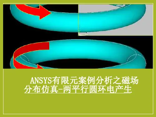
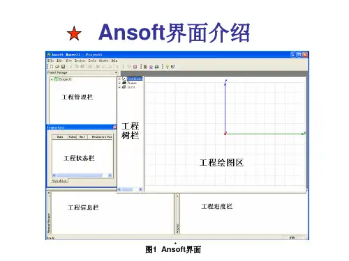
Ansoft简明教程 磁场分析实例
- 格式:ppt
- 大小:2.71 MB
- 文档页数:32

A n s o f t M a x w e l l静态磁场参数化操作
Ansoft Maxwell静态磁场参数化操作第一步、新建一个3D Design,点击下图蓝色图标
第二部、定义求解类型,默认为静磁场求解器
第三步、绘制几何模型
第四步、定义材料
第五步、添加电流激励,选中绘制的电流截面,右击Excitations——Assign——Current,在Value中设定安匝数,可将电流设成变量以便进行参数化计算,如下图将其设为I,匝数为60,并勾选Standed
第六步、添加求解参数,选中几何模型衔铁,右击Parameters,选择Force,求解完后即在可Result中查看衔铁所受电磁力
第七步、添加求解设置,右击Analysis,选择Add Solution Setup,默认设置即可,直接确定
第八步、设置参数化求解,右击Optimetrics——Add——Parametric,弹出下面对话框(图2),点Add,之后在弹出的对话框中(图3),Variable选中要进行参数化计算的变量,如电流,并在下面设置变量范围和步长,然后点Add——OK。
返回上一界面图2,重复刚才操作,完成其他变量的添加,如气隙。
之后点击图2中的Table,可查看所有会计算的参数组合形式。
图1
图2
图3 第九步、检查模型
第十步、计算,查看结果。


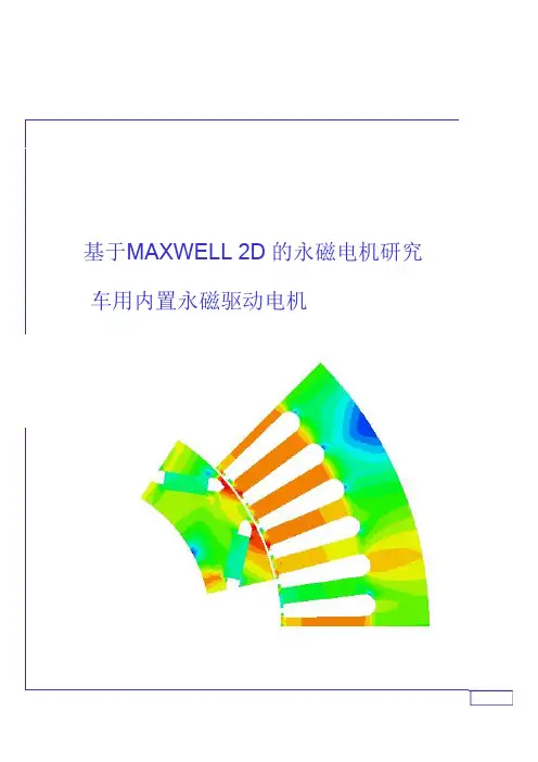
基于Ansoft Maxwell的永磁磁力耦合器磁场分析杨帆,刘露露【摘要】永磁耦合器能实现电动机和风机、泵类负载间的无机械连接传动,不仅具有调速性能,而且能实现隔振、软启动、软停止,可以适应恶劣环境。
通过三维绘图软件绘制永磁磁力耦合器的传动部件,将模型导入Ansoft Maxwell 软件进行三维静态场以及瞬态场的有限元分析,得出永磁耦合器传动部件在不同气隙下,转差和关键部件的磁密分布、电涡流密度、轴向力、输出转矩的关系,为磁力耦合器的设计制造提供理论依据。
【期刊名称】煤矿机电【年(卷),期】2019(040)003【总页数】3【关键词】永磁耦合器; Ansoft Maxwell软件;有限元分析杨帆,刘露露.基于Ansoft Maxwell的永磁磁力耦合器磁场分析[J].煤矿机电,2019,40(3):26-28.doi:10.16545/ki.cmet.2019.03.0080 引言永磁磁力耦合器是实现永磁驱动技术的一种力的传递装置,主要是采用耦合传动的原理,通过导体与永磁体(涡流式)或两个永磁体之间的非刚性接触相对运动,利用磁场穿过磁路工作气隙进行运动和动力传递,并可通过主、从动体之间气隙的调整控制传递扭矩和负载速度[1]。
国内外对于永磁磁力耦合器的设计与研究还有发展空间,目前有关永磁磁力耦合器的理论还不完备,永磁磁力耦合器设备多在实验基础上研究开发,对于永磁磁力耦合器的推广使用,需要在理论研究和技术层面进行更进一步的研究探索。
本文主要基于Ansoft Maxwell软件对永磁磁力耦合器磁场进行初步分析。
1 磁力耦合器虚拟模型建模参考国外产品目录以及实际产品应用,建立简单的永磁磁力耦合器数学模型,并在三维绘图软件中绘制耦合器的传动部件:主动部件(外钢盘、铜盘)、从动部件(内钢盘、铝盘、永磁体材料),然后将文件导入Ansoft Maxwell软件中。
由于后期做有限云分析时需要模拟模型的真实运行情况,故需要在模型的运动区域设置一个band运动区域[2]。
基于ansoft的电机磁场强度有限元计算1. Ansfot一般求解过程Ansfot一般求解过程如框图2所示。
图1 Ansfot一般求解过程图2中最重要的步骤为有限元计算,它的计算结果直接影响整个求解过程的结果分析,所以Ansfot软件是以有限元计算为核心的有限元分析软件。
2. 磁力耦合器磁场强度有限元计算第一步:选择求解器类型建立一个maxwell2D工程文件,在菜单栏中选择Solution Type,出现如下对话框,求解器类型和求解器坐标选择如下图所示图2 求解器类型和求解器坐标的选择第二步:建模用Ansoft作为仿真工具对电机进行建模时,可以在Maxwell 2D模块里直接建立完成,也可以把电机的基本设计参数填入到RMxprt中生成二维模型,其模型如下图所示图3电机平面模型第三步:设置材料属性在完成初步模型后,需要在生成的几何模型里定义电机的材料属性,其设定包括指定转轴及外层面域材料属性为空气、指定隔离套材料属性为铜和定义永磁体材料属性SmCo24第四步:设置激励源和边界条件进行瞬态场分析时,激励源为永磁体所提供此处不用给出,边界条件施加磁通平行边界条件。
图4施加磁通平行边界条件第五步:网格剖分将所有的剖分网格最大长度设置为1mm,如图5所示图5 剖分网格最大长度设置第六步:有限元计算对于有限元计算分析过程中的Analysis Setup 采用默认值。
第七步:后处理1)观察计算完后的网格剖分情况2)观察计算完后的电场强度的分布4.后处理结果1)计算完后的网格剖分情况如图6所示。
图6网格剖分情况2)磁场强度分布情况如图7所示。
a)耦合器磁力线分布情况b)耦合器磁通密度云图分布情况图7磁场强度度分布姓名:王法恒学号:1520310002专业:电气工程。
一、概述此文档介绍了利用Ansoft Maxwell2D 11.0电磁场有限元分析软件对永磁同步发电机进行磁场分析的方法,读者应先了解Ansoft软件的基本使用方法后阅读本文,Ansoft软件的基本使用方法可参阅《Ansoft工程电磁场有限元分析》(刘国强著,电子工业出版社)。
永磁同步发电机磁场分析的基本流程见图1。
图1 磁场分析的基本流程二、求解空载磁场1.绘制有限元模型(Define Model)Ansoft Maxwell2D 有限元建模的方法主要有三种,一是直接在Maxwell2D 中绘制,选择Define Model-Draw Model 进入后在软件提供的绘图界面上绘制电机模型。
二是利用Ansoft RMXpert导入,点开Maxwell 11 3D的界面,选择Project-Insert RMxpert Design,然后逐项输入电机各项数据。
输入完各项数据后,点击RMxpert-Analyze all,求解电机模型。
求解完成后,点击RMxpert-Analysis Setup-Export-Maxwell 2D Project,生成一个Maxwell 2D模型。
在弹出的对话框中,Project Name中填写模型的名字,Location填写模型存放的路径。
三是用AutoCAD绘制后导入。
将绘制后的AutoCAD图形存成*.dxf格式,在Ansoft Maxwell2D 绘图界面中点击File-Import,选中*.dxf文件在出现的设置转换参数对话框中,将Number of segments for poligonalization of a circle 和Number of segments between control points of a spline 后的数量设置得大一点,点击ok,将AutoCAD图形转换为Maxwell 2D模型图形*.sm2。
界面后选择File-Open, 打开转换好的图形。
如何利用ansoft磁路法计算生成maxwell有限元电磁计算模型如何利用ansoft中磁路法计算,一键生成maxwell有限元电磁计算模型1、以一台凸极式永磁同步电机为例:打开软件,进入下图所示截面,选中RMxprt打开选择Adjust-Speed Synchronous Machine2、进入RMxprt界面,如下图所示:3、双击Machine,出现下图界面:极数:16转子位置:内转子各种损耗:可大致设置为额定功率的2%左右额定转速:790r/min线圈交流电AC及Y3星型联接4、双击stator,出现下图界面:定子外径:250定子内径:165定子轴向长度:160叠压系数:0.97定子材料:JFE_steel_50JN800定子槽数:36定子槽型:选3斜槽数:15、双击slot,如下图示:(一开始先将Auto Design后面√去除,点确认退出,再次双击slot 进入,即出现下图设置界面)3号槽型,设置数据如上图所示6、双击winding,选择winding界面线圈层数:2线圈形式:全极式绕组线圈并联之路:2每槽导体数:38(上下两层总计数)线圈跨距:4每匝线圈数:暂时空着,系统自动计算线圈漆包厚度:0.06平均线径:单击Diameter,进入设计截面,设置如下,点击OK再选择End/Insulation界面框线圈端部长:10槽绝缘厚度:0.3楔子厚度:2层绝缘厚:0.3槽满率:0.87、双击Rotor转子外径:162.5转子内径:110转子轴向长度:160转子材料:steel_1010叠压系数:1(转子为整个铸件)磁极类型:2 8、双击pole极狐系数:0.8偏移:0(即磁钢内外径同心)磁钢材料:NdFe35 磁钢厚度:4.659、shaft轴可不设置10、右键单击Analysis单击选择Add solution setup,出现下图额定功率:17 (设置时注意单位的选择)额定电压:340额定转速:790其它默认即可11、至此RMxprt设置完成,右键点击增加的Setup1,单击Analyze 进行分析12、分析完成后可右键,可右键Results,选择Solution Data查看相关结果参数13、右键Setup1,选择Create Maxwell Design(生成有限元计算模型)选择Maxwell2D Design(或者3D,根据自己需求选择)14、系统会根据槽极比生成最小有限元单元,如此处生成1/4模型,若想生成全模型,可在RMxprt模块下,选择窗口中RMxprt,单击Design Settings,选择出现窗口下User Defined Date,设置如下(Fraction 1注意大小写及字母与数字间空一格),再点击重新计算即可生成有限元全模型谢谢!。
Example (Magnetostatic) –Magnetic Force Magnetic ForceThis example is intended to show you how to create and analyze amagnetostatic problem with a permanent magnet to determine the forceexerted on a steel bar using the Magnetostatic solver in the Ansoft Maxwell 3D Design Environment.Example (Magnetostatic) –Magnetic Force Ansoft Maxwell Design EnvironmentThe following features of the Ansoft Maxwell Design Environment are used to create the models covered in this topic3D Solid ModelingPrimitives: BoxSurface Operations: SectionBoolean Operations: Subtract, Unite, Separate BodiesBoundaries/ExcitationsCurrent: StrandedAnalysisMagnetostaticResultsForceField Overlays:Vector BExample (Magnetostatic) –Magnetic Force Getting StartedLaunching Maxwell1.To access Maxwell, click the Microsoft Start button, select Programs, and selectAnsoft and then Maxwell 11.Setting Tool OptionsTo set the tool options:Note: In order to follow the steps outlined in this example, verify that thefollowing tool options are set:1.Select the menu item Tools > Options > Maxwell Options2.Maxwell Options Window:1.Click the General Options tabUse Wizards for data entry when creating new boundaries: ;CheckedDuplicate boundaries with geometry: ;Checked2.Click the OK button3.Select the menu item Tools > Options > 3D Modeler Options.4.3D Modeler Options Window:1.Click the Operation tabAutomatically cover closed polylines: ;Checked2.Click the Drawing tabEdit property of new primitives: ;Checked3.Click the OK buttonExample (Magnetostatic) –Magnetic Force Opening a New ProjectTo open a new project:In an Ansoft Maxwell window, click the On the Standard toolbar, orselect the menu item File > New.From the Project menu, select Insert Maxwell Design.Set Solution TypeTo set the solution type:Select the menu item Maxwell > Solution TypeSolution Type Window:Choose MagnetostaticClick the OK buttonExample (Magnetostatic) –Magnetic Force Creating the 3D ModelSet Model UnitsTo set the units:1.Select the menu item 3D Modeler > Units2.Set Model Units:1.Select Units: mm2.Click the OK buttonSet Default MaterialTo set the default material:ing the 3D Modeler Materials toolbar, choose Select2.Select Definition Window:1.Type steel_1008 in the Search by Name field2.Click the OK buttonExample (Magnetostatic) –Magnetic Force Create CoreTo create a box:1.Select the menu item Draw > Boxing the coordinate entry fields, enter the box positionX: 0.0, Y: 0.0, Z: -5.0, Press the Enter keying the coordinate entry fields, enter the opposite corner of the box:dX: 10.0, dY: -30.0, dZ: 10.0, Press the Enter key To fit the view:1.Select the menu item View > Fit All > Active View.Duplicate Box:1.Select the menu item Edit > Duplicate Along Lineing the coordinate entry fields, enter the first pointX: 0.0, Y: 0.0, Z: 0.0, Press the Enter keying the coordinate entry fields, enter the second pointdX: 30.0, dY: 0.0, dZ: 10.0, Press the Enter key4.Duplicate Along Line Window1.Total Number: 22.Click the OK buttonTo create the core:1.Select the menu item Draw > Boxing the coordinate entry fields, enter the box positionX: 0.0, Y: -30.0, Z: -5.0, Press the Enter keying the coordinate entry fields, enter the opposite corner of the box:dX: 50.0, dY: -10.0, dZ: 10.0, Press the Enter key To set the name:1.Select the Attribute tab from the Properties window.2.For the Value of Name type: Core3.Click the OK buttonTo fit the view:1.Select the menu item View > Fit All > Active View.Example (Magnetostatic) –Magnetic Force Group the CoreTo select the objects1.Select the menu item Edit > Select All2.Select the menu item, 3D Modeler > Boolean > UniteTo fit the view:1.Select the menu item View > Fit All > Active View.Duplicate the CoreTo select the objects1.Select the menu item, Edit > Duplicate Mirroring the coordinate entry fields, enter the first pointX: 0.0, Y: 0.0, Z: 0.0, Press the Enter keying the coordinate entry fields, enter the normal pointdX: 0.0, dY: 1.0, dZ: 0.0, Press the Enter keyTo fit the view:1.Select the menu item View > Fit All > Active View.Group the CoreTo select the objects1.Select the menu item Edit > Select All2.Select the menu item, 3D Modeler > Boolean > UniteTo fit the view:1.Select the menu item View > Fit All > Active View.Example (Magnetostatic) –Magnetic Force Create BarTo create the bar:1.Select the menu item Draw > Boxing the coordinate entry fields, enter the box positionX: 51.0, Y: -40.0, Z: -5.0, Press the Enter keying the coordinate entry fields, enter the opposite corner of the box:dX: 10.0, dY: 80.0, dZ: 10.0, Press the Enter keyTo parameterize the object:1.Select the Command tab from the Properties window2.For Position, type: 50mm+mx, -40,0, -5,0, Click the Tab key to acceptAdd Variable mx: 1mm, Click the OK buttonTo set the name:1.Select the Attribute tab from the Properties window.2.For the Value of Name type: Bar3.Click the OK buttonTo fit the view:1.Select the menu item View > Fit All > Active View.Set Default Materialing the 3D Modeler Materials toolbar, choose Select2.Select Definition Window:1.Type copper in the Search by Name field2.Click the OK buttonExample (Magnetostatic) –Magnetic Force Create CoilTo create the coil:1.Select the menu item Draw > Boxing the coordinate entry fields, enter the box positionX: 45.0, Y: 30.0, Z: 10.0, Press the Enter keying the coordinate entry fields, enter the opposite corner of the box:dX: -20.0, dY: -60.0, dZ: -20.0, Press the Enter key To set the name:1.Select the Attribute tab from the Properties window.2.For the Value of Name type: coil3.Click the OK buttonTo select the object for subtract1.Select the menu item Edit > Select > By Name2.Select Object Dialog,1.Select the objects named: Coil, Core2.Click the OK buttonTo complete the coil:1.Select the menu item 3D Modeler > Boolean > Subtract2.Subtract Window1.Blank Parts: Coil2.Tool Parts: Core3.Clone tool objects before subtracting: ;Checked4.Click the OK buttonTo fit the view:1.Select the menu item View > Fit All > Active View.Insulate CoilTo assign a boundary1.Select the menu item Maxwell > Boundaries > Assign > Insulating2.Insulating Boundary: Insulating12.Click the OK buttonExample (Magnetostatic) –Magnetic Force Create ExcitationSection Object1.Select the menu item Edit > Surface > Section1.Section Plane: XY2.Click the OK buttonSeparate Bodies1.Select the menu item Edit > Boolean > Separate BodiesAssign Excitation1.Select the menu item Maxwell > Excitations > Assign > Current2.Current Excitation : General: Current12.Value: c13.Type: Stranded4.Current Direction: positive Z direction. (Use Swap Direction button)3.Click the OK button4.Add Variable Window1.Value: 100A2.Click the OK buttonCalculate ForceTo select the objectSelect the menu item Edit > Select > By NameSelect Object Dialog,Select the objects named: BarClick the OK buttonCalculate ForceSelect the menu item Maxwell > Parameters > Assign > ForceClick the OK buttonExample (Magnetostatic) –Magnetic ForceSet Default Materialing the 3D Modeler Materials toolbar, choose Select2.Select Definition Window:1.Type NdFe35 in the Search by Name field2.Click the OK buttonCreate MagnetTo create the magnet:1.Select the menu item Draw > Boxing the coordinate entry fields, enter the box positionX: 0.0, Y: -10.0, Z: -5.0, Press the Enter keying the coordinate entry fields, enter the opposite corner of the box:dX: 10.0, dY: 20.0, dZ: 10.0, Press the Enter key To set the name:1.Select the Attribute tab from the Properties window.2.For the Value of Name type: Magnet3.Click the OK buttonTo select the object for subtract1.Select the menu item Edit > Select > By Name2.Select Object Dialog,1.Select the objects named: Magnet, Core2.Click the OK buttonTo complete the magnet:1.Select the menu item 3D Modeler > Boolean > Subtract2.Subtract Window1.Blank Parts: Core2.Tool Parts: Magnet3.Clone tool objects before subtracting: ;Checked4.Click the OK buttonTo fit the view:1.Select the menu item View > Fit All > Active View.Example (Magnetostatic) –Magnetic ForceOrient MagnetNote: By default all of the magentic material in the material libaray are oriented in the x-direction. Using a local coordinate system (CS) we can correct the orientation of the geometry to align with the material definition.To create rotated CS:1.Select the menu item Edit > Select > Facesing the mouse, graphically select the top face of the Magnet3.Select the menu item 3D Modeler > Coordinate System > Create > Face CSing the coordinate entry fields, enter the originX: 10.0, Y: 10.0, Z: 5.0, Press the Enter keying the coordinate entry fields, enter the axis:dX: 0.0, dY: -20.0, dZ: 0.0, Press the Enter keyChange Properties1.Select the menu item Maxwell > List2.Design List Window1.From the list, select row: Magnet2.Click the Properties button3.Properties Window1.Orientation: FaceCS12.Click the OK button4.Click the Done buttonExample (Magnetostatic) –Magnetic Force Set Default MaterialTo set the default material:ing the 3D Modeler Materials toolbar, choose vacuumDefine a RegionTo define a Region:1.Select the menu item Draw > Region1.Padding Date:One2.Padding Percentage:503.Click the OK buttonExample (Magnetostatic) –Magnetic Force Analysis SetupCreating an Analysis SetupTo create an analysis setup:1.Select the menu item Maxwell > Analysis Setup > Add Solution Setup2.Solution Setup Window:1.Click the OK buttonSave ProjectTo save the project:1.In an Ansoft Maxwell window, select the menu item File > Save As.2.From the Save As window, type the Filename: maxwell_ms_magforce3.Click the Save buttonAnalyzeModel ValidationTo validate the model:1.Select the menu item Maxwell > Validation Check2.Click the Close buttonNote:To view any errors or warning messages, use the MessageManager.AnalyzeTo start the solution process:1.Select the menu item Maxwell > Analyze AllExample (Magnetostatic) –Magnetic Force Solution DataTo view the Solution Data:1.Select the menu item Maxwell > Results > Solution DataTo view the Profile:1.Click the Profile Tab.To view the Convergence:1.Click the Convergence TabNote: The default view is for convergence is Table. Selectthe Plot radio button to view a graphical representations ofthe convergence data.To view the Solutions:1.Click the Solutions Tab2.Click the Close buttonExample (Magnetostatic) –Magnetic Force Optimetrics Setup –Parametric SweepDuring the design of a device, it is common practice to develop design trendsbased on swept parameters. Ansoft Maxwell 3D with Optimetrics ParametricSweep can automatically create these design curves.Add a Parametric Sweep1.Select the menu item Maxwell > Optimetrics Analysis > Add Parametric2.Setup Sweep Analysis Window:1.Click the Sweep Definitions tab:1.Click the Add button2.Add/Edit Sweep Dialog1.Select Variable: c12.Select Linear Count3.Start: 0A4.Stop: 500A5.Step: 1006.Click the Add button7.Click the OK button2.Click the Options tab:1.Save Fields and Mesh: ;Checked3.Click the OK buttonAnalyze Parametric SweepTo start the solution process:1.Expand the Project Tree to display the items listed under Optimetrics2.Right-click the mouse on ParametricSetup1 and choose Analyze Optimetrics ResultsTo view the Optimetrics Results:1.Select the menu item Maxwell> Optimetrics Analysis > Optimetrics Results2.Select the Profile Tab to view the solution progress for each setup.3.Click the Close button when you are finished viewing the resultsExample (Magnetostatic) –Magnetic Force Create Plot of Force at each CurrentTo create a report:1.Select the menu item Maxwell > Results > Create Report2.Create Report Window:1.Report Type: Magnetostatic2.Display Type: Rectangular Plot3.Click the OK button3.Traces Window:1.Solution: Setup1: Force2.Click the Sweeps tab1.Select Sweep Design and Project variable values2.Make sure that c1is selected as the primary sweep3.Click the Y tab1.Category:Force2.Quantity: Force_x3.Function: <none>4.Click the Add Trace button4.Click the Done button。