Motion primitives for stabilization and control of underactuated vehicles

the scientific study of the motion -回复题目：The Scientific Study of MotionIntroduction:Motion is a fundamental concept studied and analyzed in various fields of science, including physics and biomechanics. The scientific study of motion involves observing, measuring, and explaining the movement of objects or bodies in relation to time, space, and forces acting upon them. In this article, we will explore thestep-by-step process involved in the scientific study of motion and delve into the principles that govern it.1. Observation:The first step in studying motion scientifically is making careful observations of objects or bodies in motion. Scientists use their senses, tools, and instruments to record data related to position, speed, and direction. By closely observing and documenting motion, researchers can identify patterns and develop hypotheses about the underlying factors contributing to the observed motion.2. Measurement:Once the observations are made, the next step is to measure therelevant quantities associated with motion. Measurements include determining the distance traveled by an object, the time taken to cover that distance, and any changes in velocity along the way. In most cases, scientists employ standardized units such as meters, seconds, and meters per second to express these measurements accurately and consistently.3. Quantitative Analysis:After gathering the necessary measurements, scientists analyze the data quantitatively. This involves utilizing mathematical equations and formulas to calculate quantities such as average speed, acceleration, and displacement. By applying mathematical models, researchers can derive valuable insights into the nature of motion and verify the underlying principles governing it.4. Formulate Hypotheses:Based on the observations and quantitative analysis, scientists formulate hypotheses to explain the observed motion. These hypotheses are testable explanations that provide a framework for further experimentation and analysis. Hypotheses may be refined or modified as new data is collected, and they serve as a starting point for the development of theories.5. Experimental Design:To test and validate the hypotheses, scientists design experiments using controlled conditions. They identify variables that may affect the motion under investigation and manipulate those variables systematically to observe the resulting changes in the motion. Experiments often involve varying factors such as force, mass, or surface conditions, while keeping other variables constant.6. Data Collection:During the experiments, scientists collect data by making precise measurements and observations. They record measurements such as displacements, velocities, accelerations, and forces, keeping a careful record of experimental conditions and any potential sources of error. The collected data is then analyzed using statistical methods to determine the significance and reliability of the results.7. Data Interpretation:Once the data is collected, scientists interpret the results to draw meaningful conclusions. They compare the observed data with the predictions made by the hypotheses under investigation. By analyzing the data in conjunction with the relevant scientificprinciples and theories, researchers can determine whether the observations align with the hypotheses or require further refinement.8. Theory Development:If the data consistently supports the hypotheses, scientists develop theories to explain the observed motion. Theories in physics, such as Newton's laws of motion, provide a comprehensive framework for understanding and predicting various types of motion. Theories help to generalize the findings beyond the specific experimental conditions and enable scientists to make predictions about motion in similar scenarios.Conclusion:The scientific study of motion involves a systematic and rigorous process that includes observation, measurement, analysis, hypothesis formulation, experimentation, data collection, interpretation, and theory development. By following these steps, scientists can gain a deeper understanding of the fundamental principles governing motion, allowing us to analyze and predict the behavior of objects and bodies in motion accurately.。

机器人顶刊论文机器人领域内除开science robotics以外，TRO和IJRR是机器人领域的两大顶刊，最近师弟在选择研究方向，因此对两大顶刊的论文做了整理。

TRO的全称IEEE Transactions on Robotics，是IEEE旗下机器人与自动化协会的汇刊，最新的影响因子为6.123。

ISSUE 61 An End-to-End Approach to Self-Folding Origami Structures2 Continuous-Time Visual-Inertial Odometry for Event Cameras3 Multicontact Locomotion of Legged Robots4 On the Combined Inverse-Dynamics/Passivity-Based Control of Elastic-Joint Robots5 Control of Magnetic Microrobot Teams for Temporal Micromanipulation Tasks6 Supervisory Control of Multirotor Vehicles in Challenging Conditions Using Inertial Measurements7 Robust Ballistic Catching: A Hybrid System Stabilization Problem8 Discrete Cosserat Approach for Multisection Soft Manipulator Dynamics9 Anonymous Hedonic Game for Task Allocation in a Large-Scale Multiple Agent System10 Multimodal Sensorimotor Integration for Expert-in-the-Loop Telerobotic Surgical Training11 Fast, Generic, and Reliable Control and Simulation of Soft Robots Using Model Order Reduction12 A Path/Surface Following Control Approach to Generate Virtual Fixtures13 Modeling and Implementation of the McKibben Actuator in Hydraulic Systems14 Information-Theoretic Model Predictive Control: Theory and Applications to Autonomous Driving15 Robust Planar Odometry Based on Symmetric Range Flow and Multiscan Alignment16 Accelerated Sensorimotor Learning of Compliant Movement Primitives17 Clock-Torqued Rolling SLIP Model and Its Application to Variable-Speed Running in aHexapod Robot18 On the Covariance of X in AX=XB19 Safe Testing of Electrical Diathermy Cutting Using a New Generation Soft ManipulatorISSUE 51 Toward Dexterous Manipulation With Augmented Adaptive Synergies: The Pisa/IIT SoftHand 22 Efficient Equilibrium Testing Under Adhesion and Anisotropy Using Empirical Contact Force Models3 Force, Impedance, and Trajectory Learning for Contact Tooling and Haptic Identification4 An Ankle–Foot Prosthesis Emulator With Control of Plantarflexion and Inversion–Eversion Torque5 SLAP: Simultaneous Localization and Planning Under Uncertainty via Dynamic Replanning in Belief Space6 An Analytical Loading Model for n -Tendon Continuum Robots7 A Direct Dense Visual Servoing Approach Using Photometric Moments8 Computational Design of Robotic Devices From High-Level Motion Specifications9 Multicontact Postures Computation on Manifolds10 Stiffness Modulation in an Elastic Articulated-Cable Leg-Orthosis Emulator: Theory and Experiment11 Human–Robot Communications of Probabilistic Beliefs via a Dirichlet Process Mixture of Statements12 Multirobot Reconnection on Graphs: Problem, Complexity, and Algorithms13 Robust Intrinsic and Extrinsic Calibration of RGB-D Cameras14 Reactive Trajectory Generation for Multiple Vehicles in Unknown Environments With Wind Disturbances15 Resource-Aware Large-Scale Cooperative Three-Dimensional Mapping Using Multiple Mobile Devices16 Control of Planar Spring–Mass Running Through Virtual Tuning of Radial Leg Damping17 Gait Design for a Snake Robot by Connecting Curve Segments and ExperimentalDemonstration18 Server-Assisted Distributed Cooperative Localization Over Unreliable Communication Links19 Realization of Smooth Pursuit for a Quantized Compliant Camera Positioning SystemISSUE 41 A Survey on Aerial Swarm Robotics2 Trajectory Planning for Quadrotor Swarms3 A Distributed Control Approach to Formation Balancing and Maneuvering of Multiple Multirotor UAVs4 Joint Coverage, Connectivity, and Charging Strategies for Distributed UAV Networks5 Robotic Herding of a Flock of Birds Using an Unmanned Aerial Vehicle6 Agile Coordination and Assistive Collision Avoidance for Quadrotor Swarms Using Virtual Structures7 Decentralized Trajectory Tracking Control for Soft Robots Interacting With the Environment8 Resilient, Provably-Correct, and High-Level Robot Behaviors9 Humanoid Dynamic Synchronization Through Whole-Body Bilateral Feedback Teleoperation10 Informed Sampling for Asymptotically Optimal Path Planning11 Robust Tactile Descriptors for Discriminating Objects From Textural Properties via Artificial Robotic Skin12 VINS-Mono: A Robust and Versatile Monocular Visual-Inertial State Estimator13 Zero Step Capturability for Legged Robots in Multicontact14 Fast Gait Mode Detection and Assistive Torque Control of an Exoskeletal Robotic Orthosis for Walking Assistance15 Physically Plausible Wrench Decomposition for Multieffector Object Manipulation16 Considering Uncertainty in Optimal Robot Control Through High-Order Cost Statistics17 Multirobot Data Gathering Under Buffer Constraints and Intermittent Communication18 Image-Guided Dual Master–Slave Robotic System for Maxillary Sinus Surgery19 Modeling and Interpolation of the Ambient Magnetic Field by Gaussian Processes20 Periodic Trajectory Planning Beyond the Static Workspace for 6-DOF Cable-Suspended Parallel Robots1 Computationally Efficient Trajectory Generation for Fully Actuated Multirotor Vehicles2 Aural Servo: Sensor-Based Control From Robot Audition3 An Efficient Acyclic Contact Planner for Multiped Robots4 Dimensionality Reduction for Dynamic Movement Primitives and Application to Bimanual Manipulation of Clothes5 Resolving Occlusion in Active Visual Target Search of High-Dimensional Robotic Systems6 Constraint Gaussian Filter With Virtual Measurement for On-Line Camera-Odometry Calibration7 A New Approach to Time-Optimal Path Parameterization Based on Reachability Analysis8 Failure Recovery in Robot–Human Object Handover9 Efficient and Stable Locomotion for Impulse-Actuated Robots Using Strictly Convex Foot Shapes10 Continuous-Phase Control of a Powered Knee–Ankle Prosthesis: Amputee Experiments Across Speeds and Inclines11 Fundamental Actuation Properties of Multirotors: Force–Moment Decoupling and Fail–Safe Robustness12 Symmetric Subspace Motion Generators13 Recovering Stable Scale in Monocular SLAM Using Object-Supplemented Bundle Adjustment14 Toward Controllable Hydraulic Coupling of Joints in a Wearable Robot15 Geometric Construction-Based Realization of Spatial Elastic Behaviors in Parallel and Serial Manipulators16 Dynamic Point-to-Point Trajectory Planning Beyond the Static Workspace for Six-DOF Cable-Suspended Parallel Robots17 Investigation of the Coin Snapping Phenomenon in Linearly Compliant Robot Grasps18 Target Tracking in the Presence of Intermittent Measurements via Motion Model Learning19 Point-Wise Fusion of Distributed Gaussian Process Experts (FuDGE) Using a Fully Decentralized Robot Team Operating in Communication-Devoid Environment20 On the Importance of Uncertainty Representation in Active SLAM1 Robust Visual Localization Across Seasons2 Grasping Without Squeezing: Design and Modeling of Shear-Activated Grippers3 Elastic Structure Preserving (ESP) Control for Compliantly Actuated Robots4 The Boundaries of Walking Stability: Viability and Controllability of Simple Models5 A Novel Robotic Platform for Aerial Manipulation Using Quadrotors as Rotating Thrust Generators6 Dynamic Humanoid Locomotion: A Scalable Formulation for HZD Gait Optimization7 3-D Robust Stability Polyhedron in Multicontact8 Cooperative Collision Avoidance for Nonholonomic Robots9 A Physics-Based Power Model for Skid-Steered Wheeled Mobile Robots10 Formation Control of Nonholonomic Mobile Robots Without Position and Velocity Measurements11 Online Identification of Environment Hunt–Crossley Models Using Polynomial Linearization12 Coordinated Search With Multiple Robots Arranged in Line Formations13 Cable-Based Robotic Crane (CBRC): Design and Implementation of Overhead Traveling Cranes Based on Variable Radius Drums14 Online Approximate Optimal Station Keeping of a Marine Craft in the Presence of an Irrotational Current15 Ultrahigh-Precision Rotational Positioning Under a Microscope: Nanorobotic System, Modeling, Control, and Applications16 Adaptive Gain Control Strategy for Constant Optical Flow Divergence Landing17 Controlling Noncooperative Herds with Robotic Herders18 ε⋆: An Online Coverage Path Planning Algorithm19 Full-Pose Tracking Control for Aerial Robotic Systems With Laterally Bounded Input Force20 Comparative Peg-in-Hole Testing of a Force-Based Manipulation Controlled Robotic HandISSUE 11 Development of the Humanoid Disaster Response Platform DRC-HUBO+2 Active Stiffness Tuning of a Spring-Based Continuum Robot for MRI-Guided Neurosurgery3 Parallel Continuum Robots: Modeling, Analysis, and Actuation-Based Force Sensing4 A Rationale for Acceleration Feedback in Force Control of Series Elastic Actuators5 Real-Time Area Coverage and Target Localization Using Receding-Horizon Ergodic Exploration6 Interaction Between Inertia, Viscosity, and Elasticity in Soft Robotic Actuator With Fluidic Network7 Exploiting Elastic Energy Storage for “Blind”Cyclic Manipulation: Modeling, Stability Analysis, Control, and Experiments for Dribbling8 Enhance In-Hand Dexterous Micromanipulation by Exploiting Adhesion Forces9 Trajectory Deformations From Physical Human–Robot Interaction10 Robotic Manipulation of a Rotating Chain11 Design Methodology for Constructing Multimaterial Origami Robots and Machines12 Dynamically Consistent Online Adaptation of Fast Motions for Robotic Manipulators13 A Controller for Guiding Leg Movement During Overground Walking With a Lower Limb Exoskeleton14 Direct Force-Reflecting Two-Layer Approach for Passive Bilateral Teleoperation With Time Delays15 Steering a Swarm of Particles Using Global Inputs and Swarm Statistics16 Fast Scheduling of Robot Teams Performing Tasks With Temporospatial Constraints17 A Three-Dimensional Magnetic Tweezer System for Intraembryonic Navigation and Measurement18 Adaptive Compensation of Multiple Actuator Faults for Two Physically Linked 2WD Robots19 General Lagrange-Type Jacobian Inverse for Nonholonomic Robotic Systems20 Asymmetric Bimanual Control of Dual-Arm Exoskeletons for Human-Cooperative Manipulations21 Fourier-Based Shape Servoing: A New Feedback Method to Actively Deform Soft Objects into Desired 2-D Image Contours22 Hierarchical Force and Positioning Task Specification for Indirect Force Controlled Robots。

prescribed structure motionPrescribed structure motion refers to a predetermined sequence of movements or actions to be followed in a specific order or pattern. It is commonly used in various fields such as sports, dance, martial arts, and rehabilitation therapy. This approach provides a systematic and organized way of executing movements to achieve specific goals or desired outcomes. Here, we will explore the concept of prescribed structure motion and its applications in different areas.In sports, prescribed structure motion is widely used to enhance performance and improve skills. For example, in gymnastics, athletes follow a prescribed routine with carefully choreographed movements to execute complex maneuvers on various apparatus. The prescribed structure motion helps athletes develop coordination, flexibility, and spatial awareness. Similarly, in synchronized swimming, athletes perform intricate movements in a synchronized manner, following a prescribed pattern to create a visually appealing routine.Dance, particularly classical ballet, often utilizes prescribed structure motion as well. Dancers learn a series of steps and sequences that are repeated in a specific order. This structured approach allows dancers to develop muscle memory, ensuring that the movements are executed precisely and gracefully. Prescribed structure motion in dance helps in creating harmonious and synchronized performances, while also enhancing the dancers' strength, flexibility, and overall technique.Martial arts also rely on prescribed structure motion. Whether it isin karate, kung fu, or judo, practitioners learn a specific sequence of moves and techniques that are practiced repeatedly. This structured approach not only helps martial artists develop precision and control over their movements but also aids in their self-defense skills. By following a prescribed structure motion, martial artists can react quickly and effectively in various scenarios, ensuring their safety and enabling efficient use of their skills.Prescribed structure motion also has applications in rehabilitation therapy. Physical therapists often design exercise programs that involve a specific sequence of movements to help patients recover from injuries or surgeries. This approach ensures that the affected areas are targeted appropriately, helping patients regain strength, flexibility, and mobility. By following the prescribed structure motion, patients can gradually progress towards their rehabilitation goals in a safe and structured manner.In conclusion, prescribed structure motion plays a crucial role in various fields, including sports, dance, martial arts, and rehabilitation therapy. It provides a systematic and organized approach to movements, allowing individuals to develop skills, enhance performance, and achieve desired outcomes. Whether it is in sports routines, choreographed dances, martial arts techniques, or rehabilitation exercises, prescribed structure motion offers a framework for individuals to follow, ensuring precision, synchronization, and efficiency in their movements.。

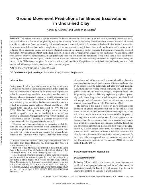
Encoding of Dynamic Visual Stimuli byPrimate Area MT NeuronsHeiko Stemmann a,∗,Winrich A.Freiwald a,Aurel Wannig a, Erich L.Schulzke b,Christian W.Eurich ba Institute for Brain Research,University of Bremen,Germanyb Institute for Theoretical Neurophysics,University of Bremen,GermanyAbstractNeural stimulus selectivity is thought to be optimized for the representation of real-world stimuli.Neural coding properties,therefore,may adapt to different envi-ronments.Here,we address the question if tuning curves depend on the statistics of visual stimuli.This is done by studying the directional tuning of macaque area MT neurons exposed to dynamic motion stimuli of two different direction progression statistics.Despite an apparent difference of tuning curves across stimulus condi-tions,our results support the view that the underlying encoding system is robust and subject to only restricted malleability by stimulus statistics.Key words:directional tuning,stimulus statistics,area MT,reverse correlation1IntroductionTuning properties in early visual cortex can be dynamic in several ways.Tun-ing curves can change within a few tens of milliseconds[1]and undergo sub-stantial changes as the result of adaptation[2]over the course of hundreds of milliseconds to seconds.Since many properties of early visual cortex can be understood in terms of an evolutionary optimization for an efficient represen-tation of natural scene statistics[3],tuning dynamics and adaptivity may be hypothesized to optimize representations within different stimulus contexts.If this is so,tuning properties ought to change with stimulus statistics.In order to address this question,we designed a novel stimulus paradigm which mimics important aspects of natural scenes:subsequent stimulus states were ∗Corresponding author:stemmann@brain.uni-bremen.dePreprint submitted to Elsevier Science22August2004determined both by a random component and a continuity requirement which dominates most of the motions we see.These stimuli were implemented as ran-dom walk trajectories in the motion direction domain,in which subsequent motion directions are correlated.Neural direction tuning obtained in this stim-ulus context was compared to tuning during stimulus sequences which only differed in the lack of any sequential correlations of motion directions.2MethodsWe conducted extracellular recordings in area MT in two male macaque mon-keys(Macaca mulatta).Surgical procedures,single-unit recording and data acquisition were standard,in short:prior to the experiments,the animals were surgically implanted with a head-holding device,a recording cylinder, and a scleral search coil.Surgical,animal care,and experimental procedures conformed to the guidelines of the National Institutes of Health for the care and use of laboratory animals,the guidelines for the welfare of experimental animals issued by the Federal Government of Germany,and stipulations of lo-cal authorities.Recordings were taken with Tungsten microelectrodes,signals amplified,filtered(350-5000Hz),digitized(sampled at25kHz)and stored on computer disk for offline analysis.Monkeys performed afixation task,foveating a small whitefixation spot (0.13◦×0.13◦)within a3◦×3◦window,while gaze direction was monitored with the indirect scleral eye-coil method.Visual stimuli were presented on a CRT monitor at a distance of either57cm or86cm at100Hz or85Hz re-fresh rate,respectively.After appearance of thefixation spot on the otherwise dark monitor and after the monkey started foveating thefixation spot,stimuli appeared inside a circular aperture covering the classical receptivefield of the neurons under investigation.Trials in which the monkeys brokefixation be-fore the end of stimulus presentation were discarded.After each successfully completed trial the animals were rewarded with a drop of juice.Visual stimuli consisted of random-dot surfaces undergoing translational mo-tion.In both stimulus paradigms the single dot diameter was0.2◦,the dot density2dots per degree2visual angle,translation speed7◦/sec,dot lifetime was infinite,and motion coherence was100%.Motion directions were updated at a rate of50,20or10Hz.The length of individual motion sequences ranged from3to5seconds.In thefirst stimulus paradigm,an adoption of the ap-proach in[1]to the motion direction domain[4],a stochastic sequence of motion directions was created(see Fig.1A and B for illustration).The se-quence was generated by pseudo-randomly selecting a new direction out of a setςof directions,sampled in steps of30◦.Selection from the set was done with replacement.The second stimulus paradigm also drew fromς,but the difference between two subsequent motion directions was now determined by2500ms 50ms ...50ms...ABFig.1.Sketches of the two different stimulus paradigms.In both paradigms,a trial starts with a 500ms period of static presentation of the random dot stimulus followed by a translational movement for 50ms (here:leftward,indicated by the gray arrow).The only,but crucial difference between both types of stimulation is indicated for the third stimulation phase by the set of arrows,whose lengths indicate choice probabilities.While in the first,“discontinuous ”,stimulus paradigm consecutive motion directions are chosen randomly out of the set ςof directions with identical probabilities (A ),in the second,“continuous ”,paradigm the consecutive directions are chosen from a Gaussian distribution centered on the current motion direction (B ).a Gaussian distribution with mean zero and standard deviation one,thus real-izing a time-discrete random walk with fixed step size in direction space.The two stimulus paradigms will be referred to as discontinuous and continuous ,respectively.Four different stimulus sequences have been generated,referred to as trajectories ,with different starting directions (0◦,90◦,180◦and 270◦).Each stimulus sequence was repeatedly presented for 10to 20trials.In order to assess the influence of stimulus statistics on neuronal responses we calculated estimates of tuning curves and optimal linear filters for the two stimulus paradigms.Spike-Triggered-Averages (STAs)were calculated for the discontinuous stimulation by reverse correlating the spike train with the stim-ulus sequence.As the discontinuous stimulus is uncorrelated,the STA closely approximates the optimal linear filter between stimulus and response.We de-fined the response delay of each neuron as the time difference between the occurrence of a spike and the maximum value of the time-dependent variance in the STA (see Fig.2A).Tuning curves were then computed from responses within a time window centered at this delay.In order to limit the influence of preceding and subsequent motion directions on the response,we divided the analysis window into five partitions of equal length,weighting the firing rates within these partitions according to different distributions (the uniform distribution corresponds to the “standard”tuning curves).Direction indices were calculated as DI =optTK −orthTK optTK +orthTK ,where optTK (orthTK)indicates the tuning curve value at the (anti-)preferred direction.33Resultsdelay [ms]309015021027033000.020.040.060.080.10.120.140.16024−3V a r i a n c e o f t h e S T A var STA A a n g l e 30 901502102703300.020.040.060.080.10.120.14024−3v a r i a n c e o f t h e S T A var STA B Fig.2.Spike triggered averages for an exemplary MT cell,obtained during discon-tinuous stimulation.(A )was obtained with 50ms motion intervals,(B )with 20ms motion intervals.The abscissa denotes the time before a spike event,the left ordinate denotes stimulus motion direction.A column within the spike triggered average for a fixed time delay τrepresents the probability distribution (grayscaled)for the stimulus present at that delay before a spike.The white line shows the vari-ance of the STA.The solid horizontal lines depict mean variance of the STA in the interval 200ms to 100ms before a spike;dashed lines indicate the twofold standard deviation;the dashed-dotted vertical line indicates the spike timestamp.The cell shows a characteristic response latency of approx.100ms for both interval lengths.Figs.2A and B show the spike triggered average of a typical cell and illustrates the procedure for delay estimation.When a spike of this cell occurred,it had,on average,most likely been preceded by a motion direction of about 300◦ap-proximately 100ms earlier.The least likely stimulus event preceding the spike was a motion direction of about 120◦at about the same delay.The tuning behavior of the neuron depicted in Fig.2is shown in Fig.3A.General activity and directional tuning differ in the two conditions.While activity levels did not vary systematically with stimulus statistics across the population of cells,directional tuning did.The histogram in Fig.3B shows the distribution of directional indices for the whole population of 45MT neurons.The two dis-tributions’medians,continuous vs.discontinuous ,differ significantly (paired Wilcoxon test:p <0.01).Thus,when tuning curves in the two conditions are computed over the full width of one stimulus presentation window (here,50ms),directional tuning seems to be significantly more pronounced during random walk (“continuous”)stimulation.However,this tuning difference be-tween stimulus conditions depends on the choice of the analysis window (see Fig.3C).With increasing emphasis on the window’s core region,a continuous decline of the significance level for the difference between the direction in-dices is observed.What are the reasons for this effect?As the analysis window shrinks,tuning curves are constructed with fewer spikes and,thus,the accu-racy of determining the directional index may degrade,obliterating real tuning differences.A second possibility,however,is that tuning can in fact be more4anglem e a n d i r e c t i o n i n d e xFig.3.Emphasis of different partitions of analysis windows is crucial for the obtained tuning curves.(A )Tuning curves of the neuron in Fig.2for both stimulation paradigms,obtained with an analysis window of 50ms (full stimulus presentation window)and taking into account the cells response latency,obtained with STAs (see Fig.2).Solid line:continuous stimulation.Dotted line:discontinuous stimulation.Note that the continuous stimulation paradigm provides the sharper tuning curve.(B )Distribution of direction indices (DI)for all recorded neurons (n=45)and both stimulus paradigms.The mean DI obtained with the discontinuous paradigm (upper panel)is significantly lower (p <0.01,paired Wilcoxon test,see also Fig.3C)than the mean DI obtained with the continuous paradigm (lower panel),indicating that tuning sharpness is reduced in the latter condition.DIs were obtained by using the full analysis window of 50ms.(C )Significance of the difference between the mean DIs obtained with the two paradigms (ordinate)depends on the different weighting of the partitions of the 50ms-analysis-windows (abscissa).The 50ms-windows were divided in 5parts of 10ms.The numbers within the bars indicate the weighting of each of the windows partitions (see methods for details).With higher weighting of the central region,the significance level decreases,indicating that the tuning curves obtained with the two paradigms assimilate to each other.(D )Mean DIs of the population (ordinate)depend on the weighting of the windows partitions as done in (C)(abscissa).With higher weighting of the inner partitions,DIs increase both in the continuous as in the discontinuous paradigm,indicating sharper tuning curves.Note that the increase is stronger in case of the discontinuous stimulation,meaning that the differences between both paradigms decrease.(E )Tuning curves of the neuron in Fig.2for both stimulation paradigms,obtained with an analysis window of 10ms,which is located in the center of the 50ms presentation window,whereas the other partitions are discarded.Note the similarity of tuning curves in comparison to Fig.3A.accurately determined with temporally restricted analysis windows,thereby minimizing the influence of responses to preceding or subsequent stimuli.Our5data support the latter scenario.As is shown in Fig.3D directional tuning im-proves during temporal focussing of the analysis window.This improvement is more pronounced for directional tuning during discontinuous than during continuous stimulation,thereby reducing the difference in directional tuning between the two conditions.This is illustrated in Fig.3E for the example neu-ron,whose tuning curves are more similar when computed over a10ms than when computed over the full50ms(Fig.3A)window.4DiscussionWe have studied the malleability of neural tuning by stimulus statistics us-ing as a model system directionally selective neurons from macaque area MT. When exposed to direction trajectories from two different statistics,neural tuning seems to be sharper during continuous stimulation.This effect can have two explanations.First,stimulus statistics genuinely alters the tuning properties of neurons in area MT.In the continuous stimulus paradigm,i.e.,the random walk in movement direction,motion direction changes less abruptly than in the discontinuous stimulus paradigm and may better reflect physical motion we see in our natural environment.Neurons in MT may there-fore adapt better to this stimulus statistics,resulting in tuning curves that are more selective.Second,since neurons in MT integrate stimuli over time,as shown for example in Fig.2,a response at any point in time may result from the influence of more than a single stimulus.Due to the continuity constraint subsequent stimuli tend to be similar in case of continuous stimulation,but not in case of discontinuous stimulation.Therefore,sharper tuning can be ex-pected during continuous stimulation-not as a result of a genuine change of tuning characteristics,but as the result of a direct effect of stimulus statis-tics on the analysis procedure.The evidence from area MT presented here lends support to the latter explanation.Directionalfilter properties of MT neurons appear robust and may not adapt to the different stimulus statistics used in our experiment.Since prolonged presentation of a single motion direc-tion has been found to induce substantial adaptation[5]and does constitute an important characteristic of stimulus statistics,future research will need to identify the precise stimulus patterns to which the information processing sys-tem adapts and to which it does not.Ourfinding provides some constraints on the time-scale of such conditions and,furthermore,demonstrates that neural tuning curves obtained with a random stimulus sequence can be directly used to predict responses in quite different stimulus contexts. Acknowledgements.We are grateful to one anonymous referee for very useful comments on an earlier version of the manuscript.This work has been supported by SFB517,B7,of the German Science Foundation(DFG),the Hanse Institute for Advanced Study(HWK),and a FNK grant of the University of Bremen.6References[1] D.L.Ringach,M.J.Hawken,and R.Shapley,Dynamics of orientation tuningin macaque primary visual cortex,Nature387(1997)281-284.[2]V.Dragoi,J.Sharma,ler,and M.Sur,Dynamics of neuronal sensitivityin visual cortex and local feature discrimination,Nature Neuroscience5(9) (2002)883-891.[3] B.A.Olshausen,and D.J.Field,Emergence of simple-cell receptivefieldproperties by learning a sparse code for natural images,Nature381(1996) 607-609.[4] B.G.Borghuis,J.A.Perge,I,Vajda,J.A.van Wezel,W.A.van de Grind,andnkheet,The motion reverse correlation(MRC)method:A linear systems approach in the motion domain,Journal of Neuroscience Methods123 (2003)153-166.[5] A.Kohn and J.A.Movshon,Adaptation changes the direction tuning ofmacaque MT neurons Nature Neuroscience,7,(2004),764-772.Heiko Stemmann has done his undergraduate training in biology at the universitiesof Oldenburg and Bremen.In2002he earned his diploma for electrophysiological workon population coding in the visual cortex done at the University of Bremen.Since2002he is doing his PhD at the Institute for Brain Research at the University of Bremenon the neural mechanisms of attention and population coding.Winrich A.Freiwald received a PhD in1998from T¨u bingen university for electro-physiological work on neural ensemble coding in the visual cortex done at the Max-Planck-Institute for Brain Research in Frankfurt/Main.He has since been working onthe neural basis of attention,population coding,and mid-and high-level vision at theUniversity of Bremen,Massachusetts Institute of Technology,Hanse Institute for Ad-vanced Study,The Athinoula A Martinos Center for Biomedical Imaging and HarvardMedical School using multi-electrode recording and functional imaging techniques.Aurel Wannig(born in1976)studied Biology at Universities of Con-stance and Bremen.Since2002,he is doing his PhD in Bremen,where hedoes electrophysiological recordings in behaving monkeys to study neuralmechanisms of object-based attention.Erich L.Schulzke,born in1975,got his diploma in Biophysics at theUniversity of Heidelberg in2001.He currently works in the group ofProf.Schwegler and Dr.Eurich as a PhD student at the Institute of The-oretical Neurophysics at Bremen within the“SFB517Neurocognition”.His research focusses on activity waves in excitable systems and analysis ofvisual information processing.7Christian W.Eurich got his PhD in Theoretical Physics in1995from the Uni-versity of Bremen.As a postdoc,he worked in the Departments of Mathematics and Neurology at the University of Chicago and at the RIKEN Brain Institute.In2001,he held a professorship for Cognitive Neuroinformatics at the University of Osnabr¨u ck. Currently,he is Research Assistant at the Institute for Theoretical Neurophysics at the University of Bremen.His research interests include signal processing and encoding in neural populations,neural dynamics,and motor control problems.8。

JointsIdealized JointsAbout Idealized JointsIdealized joints connect two parts. The parts can be rigid bodies, Flexible bodies, or Point mass es. You can place idealized joints anywhere in your model.Note:The joints you can attach to flexible bodies depend on the version of Adams/Solver you are using (C++ or FORTRAN). In addition, Adams/Solver (C++) does not support pointmasses.For a summary of which joints and forces are supported on flexible bodies, see Table ofSupported Forces and Joints in the Adams/Flex online help. Also refer to the Adams/Flexonline help for more information on attaching joints and forces to flexible bodies. Adams/View supports two types of idealized joints: simple and complex. Simple joints directly connect bodies and include the following:•Revolute Joints. See Revolute Joint Tool.•Translational Joints. See Translational Joint Tool.•Cylindrical Joints. See Cylindrical Joint Tool.•Spherical Joints. See Spherical Joint Tool.•Planar Joints. See Planar Joint Tool.•Constant-Velocity Joints. See Constant-Velocity Joint Tool.•Screw Joints. See Screw Joint Tool.•Fixed Joints. See Fixed Joint Tool.•Hooke/Universal Joint. See Hooke/Universal Joint Tool.Complex joints indirectly connect parts by coupling simple joints. They include:•Gears. See Gear Joint Tool.•Couplers. See Coupler Joint Tool.You access the joints through the Joint Palette and Joint and Motion Tool Stacks.Creating Idealized JointsThe following procedure explains how to create a simple idealized joint. You can select to attach the joint to parts or spline curves. If you select to attach the joint to a curve, Adams/View creates a curve marker,Adams/View2Jointsand the joint follows the line of the curve. Learn more about curve markers with Marker Modify dialogbox help. Attaching the joint to a spline curve is only available with Adams/Solver (C++). L earn aboutswitching solvers with Solver Settings - Executable dialog box help.Note that this procedure only sets the location and orientation of the joint. If you want to set the frictionof a joint, change the pitch of a screw joint, or set initial conditions for joints, modify the joint.To create a simple idealized joint:1.From the Joint palette or tool stack, select the joint tool representing the idealized joint that youwant to create.2.In the settings container, specify how you want to define the bodies the joint connects. You canselect:• 1 Location (Bodies Implicit)• 2 Bodies - 1 Location• 2 Bodies - 2 LocationsFor more on the effects of these options, see the help for the joint tool you are creating andConnecting Constraints to Parts.3.In the settings container, specify how you want the joint oriented. You can select:•Normal to Grid - Lets you orient the joint along the current Working grid, if it is displayed, or normal to the screen.•Pick Geometry Feature - Lets you orient the joint along a direction vector on a feature in your model, such as the face of a part.4.If you selected to explicitly define the bodies by selecting 2 Bodies - 1 Location or 2 Bodies - 2Locations in Step 2, in the settings container, set First Body and Second Body to how you wantto attach the joint: on the bodies of parts, between a part and a spline curve, or between two splinecurves.ing the left mouse button, select the first part or a spline curve (splines and data element curvesare all considered curves). If you selected to explicitly select the parts to be connected, select thesecond part or another curve using the left mouse button.6.Place the cursor where you want the joint to be located (for a curve this is referred to as its curvepoint), and click the left mouse button. If you selected to specify its location on each part or curve,place the cursor on the second location, and click the left mouse button.7.If you selected to orient the joint along a direction vector on a feature, move the cursor around inyour model to display an arrow representing the direction along a feature where you want the jointoriented. When the direction vector represents the correct orientation, click the left mouse button.Modifying Basic Properties of Idealized JointsYou can change several basic properties about an Idealized joints. These include:•Parts that the joint connects. You can also switch which part moves relative to another part.3Joints •What type of joint it is. For example, you can change a revolute joint to a translational joint. Thefollowing are exceptions to changing a joint's type:•You can only change a simple idealized joint to another type of simple idealized joint or to a joint primitive.•You cannot change a joint's type if motion is applied to the joint. In addition, if a joint has friction and you change the joint type, Adams/View displays an error.•Whether or not forces that are applied to the parts connected by the joint appear graphically on the screen during an animation. Learn about Setting Up Force Graphics.•For a screw joint, you can also set the pitch of the threads of the screw (translational displacement for every full rotational cycle). Learn about screw joints.To change basic properties for a joint:1.Display the Modify Joint dialog box as explained in Accessing Modify Dialog Boxes.2.If desired, in the First Body and Second Body text boxes, change the parts that the joint connects.The part that you enter as the first body moves relative to the part you enter as the second body.3.Set Type to the type of joint to which you want to change the current joint.4.Select whether you want to display force graphics for one of the parts that the joint connects.5.For a screw joint, enter its pitch value (translational displacement for every full rotational cycle).6.Select OK.About Initial Conditions for JointsYou can specify initial conditions for revolute, translational, and cylindrical joints. Adams/View uses the initial conditions during an Initial conditions simulation, which it runs before it runs a simulation of your model.You can specify the following initial conditions for revolute, translational, and cylindrical joints:•Translational or rotational displacements that define the translation of the location of the joint on the first part (I marker) with respect to its location on the second part (J marker) in units oflength. You can set translational displacement on a translational and cylindrical joint and you can set rotational displacements on a revolute and cylindrical joint.Adams/View measures the translational displacement at the origin of the I marker along thecommon z-axis of the I and J markers and with respect to the J marker. It measures the rotational displacement of the x-axis of the I marker about the common z-axis of the I and J markers with respect to the x-axis of the J marker.•Translational or rotational velocity that define the velocity of the location of the joint on the first part (I marker) with respect to its location on the second part (J marker) in units of length per unit of time.Adams/View Joints 4Adams/View measures the translational velocity of the I marker along the common z-axis of I and J and with respect to the J marker. It measures the rotational velocity of the x-axis of the I marker about the common z-axis of the I and J markers with respect to the x-axis of the J marker.If you specify initial conditions, Adams/View uses them as the initial velocity of the joint during an assemble model operation regardless of any other forces acting on the joint. You can also leave some or all of the initial conditions unset. Leaving an initial condition unset lets Adams/View calculate the conditions of the part during an assemble model operation depending on the other forces acting on the joint. Note that it is not the same as setting an initial condition to zero. Setting an initial condition to zero means that the joint will not be moving in the specified direction or will not be displaced when the model is assembled, regardless of any forces acting on it.If you impose initial conditions on the joint that are inconsistent with those on a part that the joint connects, the initial conditions on the joint have precedence over those on the part. If, however, you impose initial conditions on the joint that are inconsistent with imparted motions on the joint, the initial conditions as specified by the motion generator take precedence over those on the joint.Setting Initial ConditionsTo modify initial conditions:1.Display the Modify Joint dialog box as explained in Accessing Modify Dialog Boxes .2.Select Initial Conditions .The Joint Initial Conditions dialog box appears. Some options in the Joint Initial Conditions dialog box are not available (ghosted) depending on the type of joint for which you are setting initial conditions.3.Set the translational or rotational displacement or velocity, and then select OK .Imposing Point Motion on a JointYou can impose a motion on any of the axes (DOF) of the idealized joint that are free to move. For example, for a translational joint , you can apply translational motion along the z-axis. Learn more About Point Motion .Note:If the initial rotational displacement of a revolute or cylindrical joint varies by anywherefrom 5 to 60 degrees from the actual location of the joint, Adams/Solver issues a warningmessage and continues execution. If the variation is greater than 60 degrees, Adams/Viewissues an error message and stops execution.Note:For translational, revolute , and cylindrical joints, you might find it easier to use the jointmotion tools to impose motion. Learn about Creating Point Motions Using the Motion Tools .5JointsTo impose motion on a joint:1.Display the Modify Joint dialog box as explained in Accessing Modify Dialog Boxes.2.Select Impose Motion.The Impose Motion(s) dialog box appears. Some options in the Impose Motion dialog box are not available (ghosted) depending on the type of joint on which you are imposing motion.3.Enter a name for the motion. Adams/View assigns a default name to the motion.4.Enter the values for the motion as explained in Options for Point Motion Dialog Box, and thenselect OK.Adding Friction to Idealized JointsYou can model both static (Coulomb) and dynamic (viscous) friction in revolute, translational, cylindrical, hooke/universal, and spherical joints.Note:Using Adams/Solver (C++), you can apply joint friction to joints if they are attached to flexible bodies; using Adams/Solver (FORTRAN), you cannot. In addition, Adams/Solver(C++) does not support point masses.For a summary of which joints and forces are supported on flexible bodies, see Table ofSupported Forces and Joints in the Adams/Flex online help. Also refer to the Adams/Flexonline help for more information on attaching joints and forces to flexible bodies.To add friction to a joint:1.Display the Modify Joint dialog box as explained in Accessing Modify Dialog Boxes.2.Select the Friction tool .The Create/Modify Friction dialog box appears. The options in the dialog box change depending on the type of joint for which you are adding friction.3.Enter the values in the dialog box for the type of joint as explained below, and then select OK.•Cylindrical Joint Options•Revolute Joint Options•Spherical Joint Options•Translational Joint Options•Universal/Hooke Joint OptionsAdams/View6JointsFriction Regime Determination (FRD)Three friction regimes are allowed in Adams/View:diagram of the friction regimes available in Adams/Solver.7JointsConventions in Friction Block DiagramsThe following tables identify conventions used in the block diagrams:•Legend for Block Diagrams identifies symbols in the diagrams.•Relationship Between the Inputs Option and Switches Used in the Block Diagrams describes the relationship between the Input Forces to Friction option in the Create/Modify Friction dialog box and the switches used in the block diagrams.Legend for Block DiagramsRelationship Between the Inputs Option and Switches Used in the Block DiagramsCylindrical Joint frictionJoint reaction (F) and reaction torque (Tm) combined with force preload (Fprfrc) and torque preload (Tprfrc) yield the frictional force and torque in a cylindrical joint. As the block diagram indicates, you can turn off one or more of these force effects using switches SW1 through SW3. The frictional force inSymbol:Description: Scalar quantityVector quantitySumming junction:c=a+bMultiplication junction:c=axbMAGMagnitude of a vector quantity ABSAbsolute value of a scalar quantity FRD Friction regime determinationSwitch:Inputs are: Symbol: Acceptable values:SW1Preload Fprfrc or Tprfc On or offSW2Reaction force f or F On or off SW3Bending moment Tr On or off SW4 Torsional moment Tn On or off All or None sets all applicable switches On or off, respectivelyAdams/View8Jointsa cylindrical joint acts at the mating surfaces of the joint. The FRD block determines the direction of thefrictional force. Based on the frictional coefficient direction, the surface frictional force is broken downinto an equivalent frictional torque and frictional force acting along the common axis of translation androtation.9JointsCylindrical Joint OptionsFor the option: Do the following:Mu Static Define the coefficient of static friction in the joint. The magnitude of thefrictional force is the product of Mu Static and the magnitude of the normalforce in the joint, for example:Friction Force Magnitude, F = µNwhere µ = Mu Static and N = normal forceThe static frictional force acts to oppose the net force or torque along theDegrees of freedom of the joint.The range is > 0.Mu Dynamic Define the coefficient of dynamic friction. The magnitude of the frictionalforce is the product of Mu Dynamic and the magnitude of the normal forcein the joint, for example:Friction force magnitude, F = µNwhere µ = Mu Dynamic and N = normal forceThe dynamic frictional force acts in the opposite direction of the velocityof the joint.The range is > 0.Initial Overlap Defines the initial overlap of the sliding parts in either a translational orcylindrical joint. The joint's bending moment is divided by the overlap tocompute the bending moment's contribution to frictional forces.The default is 1000.0, and the range is Initial Overlap > 0.Adams/View Joints 10Overlap To define friction in a cylindrical joint, Adams/Solver computes the overlapof the joint. As the joint slides, the overlap can increase, decrease, or remainconstant. You can set:•Increase indicates that overlap increases as the I marker translates in the positive direction along the J marker; the slider moves to be within thejoint.•Decrease indicates that the overlap decreases with positive translationof the joint; the slider moves outside of the joint.•Remain Constant indicates that the amount of overlap does not changeas the joint slides; all of the slider remains within the joint.The default is Remain Constant.Pin Radius Defines the radius of the pin for a cylindrical joint.The default is 1.0, and the range is > 0.Stiction TransitionVelocity Define the absolute velocity threshold for the transition from dynamic friction to static friction. If the absolute relative velocity of the joint markeris below the value, then static friction or stiction acts to make the joint stick.The default is 0.1 length units/unit time on the surface of contact in thejoint, and the range is > 0.Max StictionDeformation Define the maximum displacement that can occur in a joint once the frictional force in the joint enters the stiction regime. The slightdeformation allows Adams/Solver to easily impose the Coulombconditions for stiction or static friction, for example:Friction force magnitude < static * normal forceTherefore, even at zero velocity, you can apply a finite stiction force if yoursystem dynamics require it.The default is 0.01 length units, and the range is > 0.Friction Force Preload Define the joint's preload frictional force, which is usually caused bymechanical interference in the assembly of the joint.Default is 0.0, and the range is > 0.Friction Torque Preload Define the preload friction torque in the joint, which is usually caused bymechanical interference in the assembly of the joint.The default is 0.0, and the Range is > 0.For the option:Do the following: 搭接接头丠丠JointsFor the option: Do the following:Effect Define the frictional effects included in the friction model, either Stictionand Sliding, Stiction, or Sliding. Stiction is static-friction effect, whileSliding is dynamic-friction effect. Excluding stiction in simulations thatdon't require it can greatly improve simulation speed. The default isStiction and Sliding.Input Forces to Friction Define the input forces to the friction model. By default, all user-definedpreloads and joint-reaction force and moments are included. You cancustomize the friction-force model by limiting the input forces you specify.The inputs for a translational joint are:•Preload•Reaction Force•Bending MomentFriction Inactive During Specify whether or not the frictional forces are to be calculated during aStatic equilibrium or Quasi-static simulation.Revolute Joint FrictionJoint reactions (Fa and Fr), bending moment (Tr), and torque preload (Tprfrc) determine the frictional torque in a revolute joint. You can turn off one or more of these force effects using switches SW1 through SW3. The joint reactions (Fa and Fr) are converted into equivalent torques using the respective friction arm (Rn) and pin radius (Rp). The joint bending moment (Tr) is converted into an equivalent torque usingpin radius (Rp) divided by bending reaction arm (Rb). The frictional torque (Tfrict) is applied along the axis of rotation in the direction that the FRD block computes.Joints Revolute Joint OptionsFor the option: Do the following:Mu Static Define the coefficient of static friction in the joint. The magnitude of thefrictional force is the product of Mu Static and the magnitude of the normalforce in the joint, for example:Friction Force Magnitude, F = µNwhere µ = Mu Static and N = normal forceThe static frictional force acts to oppose the net force or torque along theDegrees of freedom of the joint.The range is > 0.Mu Dynamic Define the coefficient of dynamic friction. The magnitude of the frictionalforce is the product of Mu Dynamic and the magnitude of the normal forcein the joint, for example:Friction force magnitude, F = µNwhere µ = Mu Dynamic and N = normal forceThe dynamic frictional force acts in the opposite direction of the velocityof the joint.The range is > 0.Friction Arm Define the effective moment arm used to compute the axial component ofthe friction torque. The default is 1.0, and the range is > 0.Bending Reaction Arm Define the effective moment arm use to compute the contribution of thebending moment on the net friction torque in the revolute joint. The defaultis 1.0, and the range is > 0.Pin Radius Defines the radius of the pin.The default is 1.0, and the range is > 0.Stiction Transition Velocity Define the absolute velocity threshold for the transition from dynamic friction to static friction. If the absolute relative velocity of the joint marker is below the value, then static friction or stiction acts to make the joint stick. The default is 0.1 length units/unit time on the surface of contact in the joint, and the range is > 0.Max Stiction Deformation Define the maximum displacement that can occur in a joint once the frictional force in the joint enters the stiction regime. The slight deformation allows Adams/Solver to easily impose the Coulomb conditions for stiction or static friction, for example:Friction force magnitude < static * normal forceTherefore, even at zero velocity, you can apply a finite stiction force if your system dynamics require it.The default is 0.01 length units, and the range is > 0.Friction Torque Preload Define the preload friction torque in the joint, which is usually caused bymechanical interference in the assembly of the joint.The default is 0.0, and the Range is > 0.Effect Define the frictional effects included in the friction model, either Stictionand Sliding, Stiction, or Sliding. Stiction is static-friction effect, whileSliding is dynamic-friction effect. Excluding stiction in simulations thatdon't require it can greatly improve simulation speed. The default isStiction and Sliding.Input Forces to Friction Define the input forces to the friction model. By default, all user-definedpreloads and joint-reaction force and moments are included. You cancustomize the friction-force model by limiting the input forces you specify.The inputs for a translational joint are:•Preload•Reaction Force•Bending MomentFriction Inactive During Specify whether or not the frictional forces are to be calculated during aStatic equilibrium or Quasi-static simulation.For the option: Do the following:JointsSpherical Joint FrictionThe reaction force (F) and the preload frictional torque (Tprfrc) are the two forcing effects used in computing the frictional torque on a Spherical joint. The ball radius is used to compute an equivalent frictional torque. The FRD block determines the direction of the frictional torque.Spherical Joint OptionsFor the option: Do the following:Mu Static Define the coefficient of static friction in the joint. The magnitude of thefrictional force is the product of Mu Static and the magnitude of the normalforce in the joint, for example:Friction Force Magnitude, F = µNwhere µ = Mu Static and N = normal forceThe static frictional force acts to oppose the net force or torque along theDegrees of freedom of the joint.The range is > 0.Mu Dynamic Define the coefficient of dynamic friction. The magnitude of the frictionalforce is the product of Mu Dynamic and the magnitude of the normal forcein the joint, for example:Friction force magnitude, F = µNwhere µ = Mu Dynamic and N = normal forceThe dynamic frictional force acts in the opposite direction of the velocityof the joint.The range is > 0.Ball Radius Defines the radius of the ball in a spherical joint for use in friction-force andtorque calculations.The default is 1.0, and the range is > 0.Stiction Transition Velocity Define the absolute velocity threshold for the transition from dynamic friction to static friction. If the absolute relative velocity of the joint marker is below the value, then static friction or stiction acts to make the joint stick. The default is 0.1 length units/unit time on the surface of contact in the joint, and the range is > 0.JointsTranslational Joint FrictionJoint reaction force (F), bending moment (Tm), torsional moment (Tn), and force preload (Fprfrc) are used to compute the frictional force in a translational joint. You can individually turn off the force effects using switches SW1 through SW4.Max StictionDeformation Define the maximum displacement that can occur in a joint once the frictional force in the joint enters the stiction regime. The slightdeformation allows Adams/Solver to easily impose the Coulombconditions for stiction or static friction, for example:Friction force magnitude < static * normal forceTherefore, even at zero velocity, you can apply a finite stiction force if yoursystem dynamics require it.The default is 0.01 length units, and the range is > 0.Friction Torque Preload Define the preload friction torque in the joint, which is usually caused bymechanical interference in the assembly of the joint.The default is 0.0, and the Range is > 0.Effect Define the frictional effects included in the friction model, either Stictionand Sliding, Stiction, or Sliding. Stiction is static-friction effect, whileSliding is dynamic-friction effect. Excluding stiction in simulations thatdon't require it can greatly improve simulation speed. The default isStiction and Sliding.Input Forces to FrictionDefine the input forces to the friction model. By default, all user-definedpreloads and joint-reaction force and moments are included. You cancustomize the friction-force model by limiting the input forces you specify.The inputs for a translational joint are:•Preload•Reaction Force Friction Inactive During Specify whether or not the frictional forces are to be calculated during aStatic equilibrium or Quasi-static simulation .For the option:Do the following:The bending moment (Tm) is converted into an equivalent force using the Xs block. Similarly, torsional moment is converted into an equivalent joint force using the friction arm (Rn). Frictional force (Ffrict) is applied along the axis of translation in the direction that the FRD block computes.Joints Translational Joint OptionsFor the option: Do the following:Mu Static Define the coefficient of static friction in the joint. The magnitude of thefrictional force is the product of Mu Static and the magnitude of the normalforce in the joint, for example:Friction Force Magnitude, F = µNwhere µ = Mu Static and N = normal forceThe static frictional force acts to oppose the net force or torque along theDegrees of freedom of the joint.The range is > 0.Mu Dynamic Define the coefficient of dynamic friction. The magnitude of the frictionalforce is the product of Mu Dynamic and the magnitude of the normal forcein the joint, for example:Friction force magnitude, F = µNwhere µ = Mu Dynamic and N = normal forceThe dynamic frictional force acts in the opposite direction of the velocityof the joint.The range is > 0.Reaction Arm Define the effective moment arm of the joint-reaction torque about thetranslational joint's axial axis (the z-direction of the joint's J marker). Thisvalue is used to compute the contribution of the torsional moment to the netfrictional force.The default is 1.0, and the range is > 0.Initial Overlap Defines the initial overlap of the sliding parts in either a translational orcylindrical joint. The joint's bending moment is divided by the overlap tocompute the bending moment's contribution to frictional forces.The default is 1000.0, and the range is Initial Overlap > 0.Overlap To define friction in a cylindrical joint, Adams/Solver computes the overlapof the joint. As the joint slides, the overlap can increase, decrease, or remainconstant. You can set:•Increase indicates that overlap increases as the I marker translates in thepositive direction along the J marker; the slider moves to be within thejoint.•Decrease indicates that the overlap decreases with positive translationof the joint; the slider moves outside of the joint.•Remain Constant indicates that the amount of overlap does not changeas the joint slides; all of the slider remains within the joint.The default is Remain Constant.Stiction Transition Velocity Define the absolute velocity threshold for the transition from dynamic friction to static friction. If the absolute relative velocity of the joint marker is below the value, then static friction or stiction acts to make the joint stick. The default is 0.1 length units/unit time on the surface of contact in the joint, and the range is > 0.Max Stiction Deformation Define the maximum displacement that can occur in a joint once the frictional force in the joint enters the stiction regime. The slight deformation allows Adams/Solver to easily impose the Coulomb conditions for stiction or static friction, for example:Friction force magnitude < static * normal forceTherefore, even at zero velocity, you can apply a finite stiction force if your system dynamics require it.The default is 0.01 length units, and the range is > 0.Friction Force Preload Define the joint's preload frictional force, which is usually caused bymechanical interference in the assembly of the joint.Default is 0.0, and the range is > 0.Effect Define the frictional effects included in the friction model, either Stictionand Sliding, Stiction, or Sliding. Stiction is static-friction effect, whileSliding is dynamic-friction effect. Excluding stiction in simulations thatdon't require it can greatly improve simulation speed. The default isStiction and Sliding.For the option: Do the following:。

motiongraphicMotion Graphic: Exploring the Dynamic World of Visual StorytellingIntroduction:Motion graphics have become an integral part of multimedia presentations, advertising campaigns, and various other forms of visual communication. This dynamic technique combines graphic design, animation, and cinematography to create engaging and informative content. From online videos to broadcast design, motion graphics play a significant role in capturing the attention of viewers and conveying complex messages in a visually appealing manner. This document aims to delve into the world of motion graphics, exploring its history, techniques, and applications.Chapter 1: The Evolution of Motion Graphics1.1 Early BeginningsMotion graphics trace their roots back to the early days of cinema and film production. Filmmakers began experimenting with visual effects and animation techniques inthe early 20th century, laying the foundation for what would eventually become motion graphics.1.2 Emergence of Computer GraphicsThe advent of computer graphics and digital technology revolutionized the field of motion graphics. With the rise of desktop computing power, animators gained access to powerful software tools that allowed for more sophisticated and complex motion graphics creation.1.3 Development of Motion GraphicsThe development of motion graphics as a distinct field can be attributed to advancements in computer technology, software capabilities, and the increasing demand for visually engaging content across various industries.Chapter 2: Techniques and Tools in Motion Graphic Design2.1 Animation PrinciplesMotion graphics rely on various animation principles, such as timing, easing, and staging, to create visually compelling and smooth movement. Understanding these principles is essential for designers to effectively communicate their ideas.2.2 Typography in Motion GraphicsIncorporating typography into motion graphics adds an additional layer of visual interest. Proper font selection, hierarchy, and animation techniques can create stunning typography-based animations that captivate the audience.2.3 Effects and TransitionsMotion graphics often utilize effects and transitions to enhance the visual impact. Techniques such as masking, layering, and compositing enable designers to seamlessly transition between scenes or convey complex ideas through visual metaphors.Chapter 3: Applications of Motion Graphics3.1 Advertising and MarketingMotion graphics have become a vital tool for advertising agencies and marketers to communicate brand messages effectively. From television commercials to online banner ads, motion graphics captivate audiences and leave a lasting impression.3.2 Film and TelevisionMotion graphics enhance visual storytelling in films and television shows. Opening titles, lower-thirds, and special effects are just a few examples of how this technique is utilized in the industry.3.3 User Interface DesignMotion graphics also play an essential role in user interface design. Interactive animations and transitions guide users through digital experiences, making interfaces more intuitive, engaging, and user-friendly.Chapter 4: Future Trends and Challenges4.1 Advancements in TechnologyAs technology continues to evolve, motion graphics will undoubtedly benefit from improved tools and software capabilities. Real-time rendering and virtual reality are poised to revolutionize the field, providing designers with new creative possibilities.4.2 Balancing Aesthetics and AccessibilityWhile motion graphics are visually captivating, maintaining accessibility for all users is crucial. Designers must strike a balance between aesthetic appeal and ensuring content is accessible for individuals with disabilities.4.3 Exploring Non-Linear StorytellingThe evolving landscape of motion graphics paves the way for non-linear storytelling, allowing viewers to interact with content and determine their own narrative path. This exciting development opens up new avenues for creativity and audience engagement.Conclusion:Motion graphics continue to make a significant impact across various industries, transforming the way we consume visual content. From humble beginnings to cutting-edge technology, this document has explored the evolution of motion graphics, its techniques, applications, and future possibilities. As technology advances and storytelling techniques evolve, motion graphics are poised to become an even more powerful tool for visual communication.。

NEW PRODUCT NEW TECHNOLOGY0 引言伴随着工业及科技领域的蓬勃发展，中国对航空航天、核工业等战略性产业愈加重视。

在这些工业场景中，工作人员通常需要在极端、危险的条件下进行作业，对人身体健康会产生较大危害。

为此，可替代技术人员进入此类极端工业场景完成复杂工作任务的智能机器人应运而生，其末端执行器的选择直接影响了机器人的工作效率。

作为结合了仿生学新型末端执行器[1，2]的灵巧手，拥有灵巧性高、适应性强、可完成多种不同类型的复杂操作等优点，成为近年来机器人领域研究的热点。

仿人灵巧手可分为全驱动仿人灵巧手和欠驱动仿人灵巧手[3-7]2类。

针对欠驱动灵巧手的发展和研究，美国宇航局（NASA）对在航天领域应用的空间机器人研制了早期最为经典的一种欠驱动灵巧手Robonaut Hand[8]，此后又与通用汽车合作对上一代灵巧手进行优化研制了第二代Robonaut Hand。

Catalano M G等[9]研制了PISA/IIT SoftHand，这种手仅用单一舵机驱动整个具有19个自由度的灵巧手，其很好地利用了腱绳驱动方式的优势，为腱绳驱动灵巧手提供了思路。

徐昱琳等[10]研制的SHU-Ⅱ采用轻质腱绳驱动并将6个直流电动机内置于手掌，其中5个电动机分别控制各手指弯曲运动，余下的1个电动机控制拇指侧摆，具有较大的运动抓取空间。

基于此，本文设计了一种腱绳驱动仿人灵巧手，先对其进行运动学分析，再求出其雅克比矩阵，分析手指动力学性能和运动空间，为仿人灵巧手提供控制依据和理论。

1 仿人灵巧手的总体设计本文灵巧手依据人手作为仿生对象，根据人体手部腱绳驱动仿人灵巧手运动分析王峥宇1 张 立1 陈耀轩1 梅 杰1，2 陈定方1，21武汉理工大学交通与物流工程学院 武汉 430063 2武汉理工大学智能制造与控制研究所 武汉 430063摘 要：针对在极端环境下代替人工进行作业的需求，文中设计了一种由腱绳驱动的灵巧手作为高效机器人末端执行器。

continental motion托福阅读"Continental motion" refers to the movement of the Earth's tectonic plates, specifically the movement of plates that are located on continental landmasses. This motion is a result of the process known as plate tectonics, which explains how the Earth's lithosphere (the outermost rigid layer of the Earth) is divided into several large and small plates that float and move on the semi-fluid asthenosphere beneath them.The movement of continental plates can result in various geological phenomena such as the formation of mountains, earthquakes, and the creation of ocean basins. These continental plates can collide and form convergent boundaries, where one plate is forced beneath another in a process called subduction. This can lead to the formation of mountain ranges like the Himalayas.Continental motion can also create divergent boundaries, where plates move apart from each other. This can result in the formation of rift valleys such as the East African Rift System. Additionally, plates can slide past each other along transform boundaries, resulting in horizontal movement and causing earthquakes, such as the San Andreas Fault in California.Understanding continental motion is important for geologists and scientists as it helps explain the dynamic nature of the Earth's surface and how different geological features and events occur.。