ANSYS稳态热分析的基本过程和实例

ANSYS 稳态和瞬态热模拟基本步骤基于ANSYS 9.0一、稳态分析从温度场是否是时间的函数即是否随时间变化上，热分析包括稳态和瞬态热分析。

其中，稳态指的是系统的温度场不随时间变化，系统的净热流率为0，即流入系统的热量加上系统自身产生的热量等于流出系统的热量：=0q q q+-流入生成流出在稳态分析中，任一节点的温度不随时间变化。

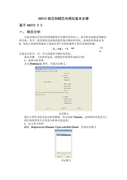
基本步骤：（为简单起见，按照软件的菜单逐级介绍）1、选择分析类型点击Preferences 菜单，出现对话框1。

对话框1我们主要针对的是热分析的模拟，所以选择Thermal 。

这样做的目的是为了使后面的菜单中只有热分析相关的选项。

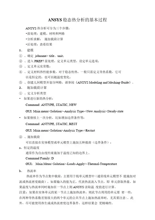
2、定义单元类型GUI ：Preprocessor>Element Type>Add/Edit/Delete 出现对话框2对话框2（3-1）点击Add,出现对话框3对话框3在ANSYS中能够用来热分析的单元大约有40种，根据所建立的模型选择合适的热分析单元。

对于三维模型，多选择SLOID87：六节点四面体单元。

3、选择温度单位默认一般都是国际单位制，温度为开尔文（K）。

如要改为℃，如下操作GUI：Preprocessor>Material Props>Temperature Units选择需要的温度单位。

4、定义材料属性对于稳态分析，一般只需要定义导热系数，他可以是恒定的，也可以随温度变化。

GUI: Preprocessor>Material Props> Material Models 出现对话框4对话框4一般热分析，材料的热导率都是各向同性的，热导率设定如对话框5.对话框5若要设定材料的热导率随温度变化，主要针对半导体材料。

则需要点击对话框5中的Add Temperature选项，设置不同温度点对应的热导率，当然温度点越多，模拟结果越准确。

设置完毕后，可以点击Graph按钮，软件会生成热导率随温度变化的曲线。

ANSYS稳态热分析的基本过程ANSYS热分析可分为三个步骤：•前处理：建模、材料和网格•分析求解：施加载荷计算•后处理：査看结果1、建模①、确定jobname> title、unit；②、进入PREP7前处理，定义单元类型，设定单元选项；③、定义单元实常数；④、定义材料热性能参数，对于稳态传热，一般只需定义导热系数，它可以是恒定的，也可以随温度变化；⑤、创建儿何模型并划分网格，请参阅《ANSYS Modeling and Meshing Guide》。

2、施加载荷计算①、定义分析类型•如果进行新的热分析：Command: ANTYPE, STATIC, NEWGUI: Main menu>Solution>-Analysis Type->New Analysis>Steady-state•如果继续上一次分析，比如增加边界条件等：Command: ANTYPE, STATIC, RESTGUI: Main menu>Solution>Analysis Type->Restart②、施加载荷可以直接在实体模型或单元模型上施加五种载荷（边界条件）：a、恒定的温度通常作为自由度约束施加于温度已知的边界上。

Command Family: DGUI： Main Menu>Solution>-Loads-Apply>-Thermal-Temperatureb、热流率热流率作为节点集中载荷，主要用于线单元模型中（通常线单元模型不能施加对流或热流密度载荷），如果输入的值为正，代表热流流入节点，即单元获取热量。

如果温度与热流率同时施加在一节点上则ANSYS读取温度值进行计算。

注意：如果在实体单元的某一节点上施加热流率，则此节点周用的单元要密一些，在两种导热系数差别很大的两个单元的公共节点上施加热流率时, 尤其要注意:。

此外，尽可能使用热生成或热流密度边界条件，这样结果会更精确些。

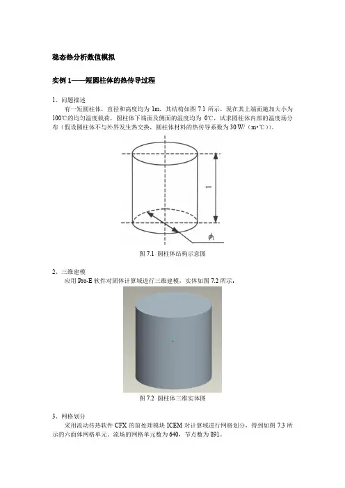
稳态热分析数值模拟实例1——短圆柱体的热传导过程1、问题描述有一短圆柱体，直径和高度均为1m，其结构如图7.1所示，现在其上端面施加大小为100℃的均匀温度载荷，圆柱体下端面及侧面的温度均为0℃，试求圆柱体内部的温度场分布（假设圆柱体不与外界发生热交换，圆柱体材料的热传导系数为30 W/（m•℃））。

图7.1 圆柱体结构示意图2、三维建模应用Pro-E软件对固体计算域进行三维建模，实体如图7.2所示：图7.2 圆柱体三维实体图3、网格划分采用流动传热软件CFX的前处理模块ICEM对计算域进行网格划分，得到如图7.3所示的六面体网格单元。

流场的网格单元数为640，节点数为891。

图7.3 圆柱体网格图4、模拟计算及结果采用流动传热软件CFX稳态计算，定义圆柱体材料的热传导系数为30 W/(m•℃)，求解时选取Thermal Energy传热模型。

固体上壁面的边界条件设置为100℃的温度，侧面和下壁面边界条件为0℃的温度。

求解方法采用高精度求解，计算收敛残差为10-4。

图7.4为计算得到的圆柱体中心剖面的温度等值线分布图。

数据文件及结果文件在steady文件夹内。

图7.4 圆柱体中心剖面的温度等值线分布瞬态热分析数值模拟实例详解实例1——型材瞬态传热过程分析1、问题描述有一横截面为矩形的型材，如图7.5所示。

其初始温度为500℃，现突然将其置于温度为20℃的空气中，求1分钟后该型材的温度场分布及其中心温度随时间的变化规律（材料性能参数如表7.1所示）。

表7.1 材料性能参数密度ρkg/m3 导热系数W/(m•℃)比热J/(kg•℃)对流系数W/(m2•℃)2400 30 352 110图7.5 型材横截面示意图2、三维建模应用Pro-E软件对固体计算域进行三维建模，实体如图7.6所示：图7.6 型材三维实体图3、网格划分采用流动传热软件CFX的前处理模块ICEM对计算域进行网格划分，得到如图7.7所示的六面体网格单元。

5.
网格
Step 5: 施加速度边界条件Apply Velocity Boundary Conditions
1.
2. 3. 4.
选择菜单路径 Utility Menu> Select> Entities. 出现对话框The Select Entities. 选择 Nodes 和 Exterior. 点击OK. 选择菜单路径 Main Menu> Preprocessor> Loads> Define Loads> Apply> Fluid/CFD> Velocity> On Nodes. 出现选择菜单 Apply V on Nodes 。
1.
5. 点击OK. 图形窗口显示下图：
1
NODAL SOLUTION STEP=4 SUB =1 TEMP (AVG) RSYS=0 SMN =280 SMX =320 APR 15 2009 16:01:45
Y Z MX X 280
MN
288.889 297.778 306.667 315.556 284.444 293.333 302.222 311.111 320 Buoyancy driven flow in a square cavity
该分析是一个层流稳态分析采用fluid1412d单该物理模型可代表一系列的实际问题包括太阳能采集房间内的空气流通等等
层流稳态热分析
------浮力驱动的流动
问题描述：
本案例模拟一个方形空穴内的浮力驱动的流动，其
垂直侧边加热条件不同。 该分析是一个层流稳态分析，采用Fluid 141 2-D单 元。 该物理模型可代表一系列的实际问题，包括太阳能 采集、房间内的空气流通等等。

ansys稳态热力学分析的基本过程及注意要点1. ansys热力学分析的基本过程及注意要点1.1，对于稳态分析，一般只需要定义导热系数，它可以是恒定的，也可以是随温度变化的。

1.2，在分析过程中，不一定选择国际单位制，但是在建立几何模型及输入材料热性参数时，单位必须统一。

2. ansys中提供6种热载荷：温度（temperature），热流率（heat flow），对流（convection），热流密度（heat flux），生热率（heat generate），辐射率（radiation）。

2.1 温度载荷2.1.1 在单个或者多个节点上施加温度载荷main menu/solution/define loads/apply/thermal/temperature/on nodes2.1.2 在所有节点上施加均匀温度载荷main menu/solution/define loads/apply/thermal/temperature/uniform tempmain menu/solution/define loads/setting /uniform tempmain menu/solution/loading options/uniform temp2.1.3 在关键点上施加温度载荷main menu/solution/define loads/apply/thermal/ temperature/on keypoints 2.1.4 在线段上施加温度载荷main menu/solution/define loads/apply/thermal/temperature/on lines2.1.5 在面上施加温度载荷main menu /solution/define loads/apply /thermal/ temperature/ on areas 2.2 热流率载荷2.2.1 在节点上施加热流率载荷main menu/solution/define loads/apply/thermal/heat flow/on nodes2.2.2 在关键点上施加热流率载荷2.3 对流载荷(convection)2.3.1在节点上施加对流载荷main menu/solution/define loads /apply/thermal/ convection/ on nodes2.3.2 在单元上施加均匀对流载荷mani menu/solution/ define loads/ apply /thermal/ convection /on elements/ uniform2.3.3 在单元上施加非均匀对流载荷mani menu/solution/ define loads/ apply /thermal/ convection /on elements/ tapered2.3.4 在线段上施加对流载荷main menu/solution/ define loads/ apply/ thermal/ convection/on lines2.3.5 在面上施加对流载荷main menu/ solution/ define loads/ apply /thermal/ convection/on areas2.4 热流密度载荷（heat flux）2.4.1 在节点上施加热流密度载荷main menu/ solution/ define loads/apply/ thermal/ heat flux/ on nodes2.4.2 在单元上施加热流密度载荷main menu/ solution/deine loads/apply thermal/heat flux / on elements2.4.3 在线段上施加热流密度载荷main menu/ solution /define loads/ apply / thermal/ heat flux/ on lines2.4.4 在面上施加热流密度载荷main menu/solution/ define loads /apply/ thermal/ heat flux/ on areas2.5 生热率载荷（heat generate）2.5.1 在节点上施加生热密度载荷main menu/solution/define loads /apply/ thermal/ heat generate/ on nodes 2.5.2 在所有节点施加均匀生热流密度载荷main menu / solution/ define loads /apply /thermal/ heat generate/ uniform heat generate2.5.3 在线段上施加生热密度载荷main menu / solution/ define loads /apply /thermal/ heat generate/on lines 2.5.4 在面上施加生热密度载荷main menu / solution/ define loads /apply /thermal/ heat generate/on areas 2.5.5 在体上施加生热密度载荷main menu / solution/ define loads /apply /thermal/ heat generate/on volumes 2.6 辐射率载荷(radiation)2.6.1 在节点上施加辐射率载荷main menu/ solution /define loads/ apply /thermal /radiation/ on Nodes2.6.2 在单元上施加辐射率载荷main menu/ solution /define loads/ apply /thermal /radiation/ on elements 2.6.3 在线段上施加辐射率载荷main menu/ solution /define loads/ apply /thermal /radiation/ on lines2.6.4 在面上施加辐射率载荷main menu/ solution /define loads/ apply /thermal /radiation/on areas3 稳态求解选项设置在对一个稳态热分析问题时，需要设置time/frequence选项、非线性选项以及输出控制等载荷步选项3.1 time-time step该选项用于设置载荷步的时间main menu/solution/loads step opts/ time&frequence/time -time step3.2 time and substeps该选项用于确定每载荷步中子步的数量或者时间步大小main menu/ solution/ load step options/ time & frequence/ time and substeps 3.3 convergence criteria该选项可根据温度、热流率等指标设置热分析的收敛标准，检验热分析的收敛性。

A N S Y S热分析指南——A N S Y S稳态热分析ANSYS热分析指南(第三章)第三章稳态热分析3.1稳态传热的定义ANSYS/Multiphysics，ANSYS/Mechanical，ANSYS/FLOTRAN和ANSYS/Professional这些产品支持稳态热分析。

稳态传热用于分析稳定的热载荷对系统或部件的影响。

通常在进行瞬态热分析以前，进行稳态热分析用于确定初始温度分布。

也可以在所有瞬态效应消失后，将稳态热分析作为瞬态热分析的最后一步进行分析。

稳态热分析可以计算确定由于不随时间变化的热载荷引起的温度、热梯度、热流率、热流密度等参数。

这些热载荷包括：对流辐射热流率热流密度（单位面积热流）热生成率（单位体积热流）固定温度的边界条件稳态热分析可用于材料属性固定不变的线性问题和材料性质随温度变化的非线性问题。

事实上，大多数材料的热性能都随温度变化，因此在通常情况下，热分析都是非线性的。

当然，如果在分析中考虑辐射，则分析也是非线性的。

3.2热分析的单元ANSYS和ANSYS/Professional中大约有40种单元有助于进行稳态分析。

有关单元的详细描述请参考《ANSYS Element Reference》，该手册以单元编号来讲述单元，第一个单元是LINK1。

单元名采用大写，所有的单元都可用于稳态和瞬态热分析。

其中SOLID70单元还具有补偿在恒定速度场下由于传质导致的热流的功能。

这些热分析单元如下：表3-1二维实体单元表3-2三维实体单元表3-3辐射连接单元表3-4传导杆单元表3-5对流连接单元表3-6壳单元表3-7耦合场单元表3-8特殊单元3.3热分析的基本过程ANSYS热分析包含如下三个主要步骤：前处理：建模求解：施加荷载并求解后处理：查看结果以下的内容将讲述如何执行上面的步骤。

首先，对每一步的任务进行总体的介绍，然后通过一个管接处的稳态热分析的实例来引导读者如何按照GUI路径逐步完成一个稳态热分析。

Guidelines
目录 （续）
第三章 稳态传热分析 一、稳态传热的定义 二、热分析的单元 三、ANSYS稳态热分析的基本过程 练习 第四章 瞬态传热分析 一、瞬态传热分析的定义 二、瞬态热分析的单元及命令 三、ANSYS瞬态热分析的主要步骤
1、建模 2、加载求解 3、后处理
四、相变问题 练习
Guidelines
系数； [C]为比热矩阵,考虑系统内能的增加; {T}为节点温度向量； { }为温度对时间的导数;
{TQ}为节点热流率向量，包含热生成。
Guidelines
第六讲、线性与非线性
如果有下列情况产生，则为非线性热分析： ①、材料热性能随温度变化，如K(T),C(T)等； ②、边界条件随温度变化，如h(T)等； ③、含有非线性单元； ④、考虑辐射传热 非线性热分析的热平衡矩阵方程为：
第三讲、热传递的方式
Definition
3、热辐射
热辐射指物体发射电磁能，并被其它物体吸收转变为热的热 量交换过程。物体温度越高，单位时间辐射的热量越多。 热传导和热对流都需要有传热介质，而热辐射无须任何 介质。实质上，在真空中的热辐射效率最高。
在工程中通常考虑两个或两个以上物体之间的辐射，系统中 每个物体同时辐射并吸收热量。它们之间的净热量传递 可以用斯蒂芬 —波尔兹曼方程来计算： q=εσA1F12(T14T24)，式中q为热流率， ε为辐射率（黑度）， σ为斯蒂芬 －波尔兹曼常数，约为5.67×10-8W/m2.K4，A1为辐射面1 的面积，F12为由辐射面1到辐射面2的形状系数，T1为辐 射面1的绝对温度，T2为辐射面2的绝对温度。由上式可 以看出，包含热辐射的热分析是高度非线性的。
线性： LINK32
两维二节点热传导单元

在操作过程中，由于不细心导致了多次重做，浪费很长的时间，若是在以后的工程项目中出现了此类问题耽误的就不只是我一个人的时间了，这教导我以后凡事都要细心仔细地去做，并且要善于与他人交流，向真，踏实平静的完成工作。
《热工基础》课程报告评分标准
评审依据
得分
评审指标1
能够了解并掌握热传导\热对流\热辐射等重点理论知识与原理。
评审指标2
能够运用传热学的基本定律和基本知识及原理，结合文献资料研究，对机械设计及制造的解决方案的各种影响因素进行分析，掌握热传导\热对流\热辐射以及综合传热等问题的基本分析方法和计算方法。
评审指标3
能够理解和评价机械产品设计\制造过程和产品运用对能源\环境等方面的影响，客观评价工程实践与能源节约问题的冲突，优化机械产品设计\制造过程问题的解决方案，采取合理的技术手段减少对环境的影响和节约资源。
总评成绩
—
教师签字：
图表6图表6二总结在操作过程中由于不细心导致了多次重做浪费很长的时间若是在以后的工程项目中出现了此类问题耽误的就不只是我一个人的时间了这教导我以后凡事都要细心仔细地去做并且要善于与他人交流向他人学习借鉴
使用ansys进行“T型管的稳态热-流-固耦合仿真分析计算”的分析流程描述与结果分析
学院：
专业：
班级：
图表2
3.第三步是流体的求解过程。
比较繁琐的就是参数的设置，但是难度不大，只需要按照教程一点一点的进行设置即可。（图表3）
图表3
4.分析处理
进行速度，温度，压力的求解。（图表4）
图表4
进行速度分析。（图表5）
图表5
进行cfd后处理，其中，不划分网格很平滑，划分后变得有梯度了。（图表6）
图表6
二、总结

ANSYS有限元分析从入门到精通7．边界条件、初始条件ANSYS热分析的边界条件或初始条件可分为七种：温度、热流率、热流密度、对流、辐射、绝热、生热。

8．热分析误差估计●仅用于评估由于网格密度不够带来的误差。

●仅适用于SOLID或SHELL的热单元（只有温度一个自由度）。

●基于单元边界的热流密度的不连续。

●仅对一种材料、线性、稳态热分析有效。

●使用自适应网格划分可以对误差进行控制。

21.2 稳态传热分析稳态传热用于分析稳定的热载荷对系统或部件的影响。

通常在进行瞬态热分析以前，进行稳态热分析以确定初始温度分布。

稳态热分析可以通过有限元计算确定由于稳定的热载荷引起的温度、热梯度、热流率、热流密度等参数。

热分析涉及到的单元有大约40种，其中纯粹用于热分析的有14种。

（1）线性。

●LINK32：两维2节点热传导单元。

●LINK33：三维2节点热传导单元。

●LINK34：二节点热对流单元。

●LINK31：二节点热辐射单元。

（2）二维实体。

●PLANE55：4节点四边形单元。

●PLANE77：8节点四边形单元。

●PLANE35：3节点三角形单元。

●PLANE75：4节点轴对称单元。

●PLANE78：8节点轴对称单元。

（3）三维实体。

●SOLID87：6节点四面体单元。

●SOLID70：8节点六面体单元。

●SOLID90：20节点六面体单元。

（4）壳（SHELL57：4节点）。

（5）点（MASS71）。

21.2.1 ANSYS稳态热分析的基本过程ANSYS热分析可分为3个步骤。

●前处理：建模。

●求解：施加载荷计算。

338。

b. 网格控制：在Details of “Mesh ” 中单击sizing，size function选择 Proximity and Curvature（临近 以及曲率）选项
c. 选中Mesh，单击鼠标右键
→Generate Mesh
c
1
稳态热分析实例
划分网格 e. 对于曲面模型使用Proximity and Curvature（临近以及曲率）网格控制会
k导热系数（W/(m·℃)），q二次导数为热流密度（W/m^2）
1
热分析简介
基本的传热方式：热传导、热对流、热辐射、相变 2. 热对流（Convection） 对流是指温度不同的各个部分流体之间发生相对运动所引起的热量传递方 式。 热对流满足牛顿冷却方程：
q" h(Ts Tb)
q"为热流密度； h为物质的对流传热系数 ； TS是固体的表面温度； Tb为周围流体温度。
（续）
1
流程简介ቤተ መጻሕፍቲ ባይዱ
材料属性
1
流程简介
装配体与接触
•对于复杂的装配体模型，如果零件初始不接触将不会互相传热
•如果初始有接触就会发生传热
•对于不同的接触类型，将会决定接触面以及目标面之间是否会发生热量传递。 可以利用pinball调整模型可能出现的 间隙，如下表所示：
接触类型
•节点位于Pinball 内：
Mechanical。选中模型树 Geometry 下模型1 2. 在Detail of “1”中，展开Material选 项，单击Assignment后三角 3. 在下拉菜单中选择Copper Alloy
1
稳态热分析实例
划分网格 a. 首先使用程序自动划分网格，查

ANSYS基础教程—热分析关键字：ANSYS ANSYS教程ANSYS热分析信息化调查找茬投稿收藏评论好文推荐打印社区分享本文简述了进行稳态热分析的过程.有两方面的目的:重申第4章所介绍的典型分析步骤；介绍热荷载与边界条件.包括的主题有：概述、分析过程、专题讨论。

A. 概述·热分析用于确定结构中温度分布、温度梯度、热流以及其它类似的量.·热分析可能是稳态的或瞬态的.–稳态是指荷载条件已被“设置”成稳定状态，几乎不随时间变化. 如: 铁获得了预先设置的温度.–瞬态* 指条件随时间变化而变化. 如: 铸造中金属从熔融状态变为固态的冷却过程.·热荷载条件可能是:温度模型区温度已知.对流表面的热传递给周围的流体通过对流。

输入对流换热系数h和环境流体的平均温度Tb热通量* 单位面积上的热流率已知的面.热流率* 热流率已知的点.热生成率* 体的生热率已知的区域.热辐射* 通过辐射产生热传递的面. 输入辐射系数, Stefan-Boltzmann常数, “空间节点”的温度作为可选项输入.绝热面“完全绝热”面，该面上不发生热传递.B. 分析过程·稳态热分析过程和静力分析类似:–分析过程·几何尺寸（模型）·划分网格–求解·荷载条件·求解–后处理·查看结果·检查结果是否正确·通过(Main Menu > Preferences)把图形用户界面的优先级设置成热分析. 前处理几何尺寸（模型）·既可用ANSYS建立模型，也可用其它方法建好模型后导入.·模型建好后，以上两种建模方法的具体过程将不再显示.-划分网格·首先定义单元属性: 单元类型, 实常数, 材料属性.-单元类型·下表给出了常用的热单元类型.·每个结点只有一个自由度: 温度常用的热单元类型-材料属性–必须输入导热系数, KXX.–如果施加了内部热生成率，则需指定比热(C).–ANSYS提供的材料库(/ansys57/matlib)包括几种常用材料的结构属性和热属性, 但是建议用户创建、使用自己的材料库.–把优先设置为“热分析”，使材料模型图形用户界面只显示材料的热属性.-实常数–主要应用于壳单元和线单元.·划分网格.–存储数据文件.–使用MeshTool划分网格. 使用缺省的智能网格划分级别6可以生成很好的初始网格.·至此完成前处理，下面开始求解.求解荷载·指定的温度–热分析的自由度约束–Solution > -Loads-Apply > Temperature–或D命令系列(DA, DL, D)·热流–这些是面荷载–Solution > -Loads-Apply > Convection–或SF命令系列(SFA, SFL, SF, SFE)·绝热面–“完全绝热”面，该面上不发生热传递.–这是缺省条件, 如,没有指定边界条件的任何一个面都被自动作为绝热面处理.·其它可能的热荷载:–热通量(BTU / (hr-in2)–热流(BTU / hr)–热生成率(BTU / (hr-in3)–热辐射(BTU / hr)求解·首先存储数据库文件.·然后输入SOLVE命令或点击菜单Solution > -Solve-Current LS.–结果被写入结果文件, jobname.rth, 该结果文件同时也写入内存中的数据库文件.·至此完成求解过程. 下面进入后处理部分.后处理查看结果·典型的等值线绘图包括温度等值线，温度梯度等值线和热通量等值线–General Postproc> Plot Results > Nodal Solu…(或Element Solu…)–或用PLNSOL(或PLESOL)·对3-D 实体模型绘制云图时，选项isosurfaces(等值面)是非常有用的. 用/CTYPE命令或Utility Menu > PlotCtrls> Style > Contours > Contour Style.·检查结果是否正确·温度是否在预期的范围内?–在指定温度和热流边界的基础上，估计预期的范围.·网格大小是否满足精度?–和受力分析一样，可以画出非均匀分布的温度梯度(单元解) 并找出高梯度的单元. 这些区域可作为重新定义网格时的参考.–若节点温度梯度（平均的）和单元温度梯度（非平均的）之间的差别很大，则可能是网格划分太粗糙.。

Workbench -Mechanical Introduction Introduction作业6.1稳态热分析作业6.1 –目标Workshop Supplement •本作业中，将分析下图所示泵壳的热传导特性。

•确切说是分析相同边界条件下的塑料（Polyethylene）泵壳和铝（Aluminum）泵壳。

）泵壳•目标是对比两种泵壳的热分析结果。

作业6.1 –假设Workshop Supplement 假设：•泵上的泵壳承受的温度为60度。

假设泵的装配面也处于60度下。

•泵的内表面承受90度的流体。

•泵的外表面环境用一个对流关系简化了的停滞空气模拟，温度为20度。

作业6.1 –Project SchematicWorkshop Supplement •打开Project 页•从Units菜单上确定：–项目单位设为Metric (kg, mm, s, C, mA, mV)–选择Display Values in Project Units…作业6.1 –Project SchematicWorkshop Supplement 1.在Toolbox中双击Steady-State Thermal创建一个新的Steady State Thermal（稳态Steady State Thermal热分析）系统。

1.2.在Geometry上点击鼠标右键选择p y，导入文Import Geometry件Pump_housing.x_t 2.…作业6.1 –Project SchematicWorkshop Supplement3.双击Engineering Data得到materialproperties（材料特性） 3.4.选中General Materials的同时，点击Aluminum Alloy和Polyethylene旁边的‘+’符号，把它们添加到项目中。

5.Return to Project（返回到项目）4.5.Workshop Supplement…作业6.1 –Project Schematic6.把Steady StateThermal 拖放到第一个系统的Geometry 上。

实例1：某一潜水艇可以简化为一圆筒，它由三层组成，最外面一层为不锈钢，中间为玻纤隔热层，最里面为铝层，筒内为空气，筒外为海水，求内外壁面温度及温度分布。

几何参数：筒外径30 feet总壁厚2 inch不锈钢层壁厚0.75inch玻纤层壁厚 1 inch铝层壁厚0.25i nch筒长200 feet导热系数不锈钢8.27BTU/hr.ft. o F玻纤0.028 BTU/hr.ft. o F铝117.4 BTU/hr.ft. o F边界条件空气温度70 o F海水温度44.5 o F空气对流系数2.5 BTU/hr.ft 2.0F海水对流系数80 BTU/hr.ft 2.o F沿垂直于圆筒轴线作横截面，得到一圆环，取其中1度进行分析，如图示。

空气'玻璃纤维、1*:不锈钢:3/+M海水R15 feet/filename ，Steady1 /title ，Steady-state thermal analysis of submarine /units ，BFT Ro=15 !外径(ft)Rss=15-(0.75/12) ! 不锈钢层内径ft) Rins=15-(1.75/12) ! 玻璃纤维层内径(ft) Ral=15-(2/12) ! 铝层内径(ft) Tair=70 ! 潜水艇内空气温度Tsea=44.5 !海水温度Kss=8.27 ! 不锈钢的导热系数(BTU/hr.ft.oF) Kins=0.028 ! 玻璃纤维的导热系数(BTU/hr.ft.oF)Kal=117.4 ! 铝的导热系数(BTU/hr.ft.oF) Hair=2.5 ! 空气的对流系数(BTU/hr.ft2.oF) Hsea=80 ! 海水的对流系数(BTU/hr.ft2.oF) prep7et，1，plane55 !定义二维热单元mp，kxx ，1，Kss !设定不锈钢的导热系数mp，kxx ，2，Kins !设定玻璃纤维的导热系数mp，kxx ，3，Kal !设定铝的导热系数pcirc，Ro，Rss，-0.5，0.5 !创建几何模型pcirc ，Rss，Rins ，-0.5 ，0.5 pcirc ，Rins，Ral，-0.5 ，0.5 aglue，all numcmp，area lesize，1，，，16 !设定划分网格密度lesize，4，，，4 lesize，14，，，5 lesize，16，，，2 Mshape，2 ! 设定为映射网格划分mat，1 amesh，1 mat，2 amesh，2 mat，3 amesh，3 /SOLUSFL，11，CONV ，HAIR ，，TAIR ! 施加空气对流边界SFL，1，CONV ，HSEA ，，TSEA !施加海水对流边界SOLVE /POST1PLNSOL ！输出温度彩色云图finish实例2一圆筒形的罐有一接管，罐外径为 3英尺，壁厚为0.2英尺，接管外径为0.5英尺，壁厚为0.1英尺，罐与接管的轴线垂直且接管远离罐的端部。

本例题的主要部分为一个圆筒形罐，其上沿径向有一材料一样的接管（如图？？？？所所示），罐内流动着450°F（232°C）的高温流体，接管内流动着100°F（38 °C）的低温流体，两个流体区域由薄壁管隔离。

罐的对流换热系数为250Btu/hr-ft2-o F（1420watts/m2-°K），接管的对流换热系数随管壁温度而变，它的热物理性能如表？？？所示。

要求计算罐与接管的温度分布。

表？？？？6.5.1 预处理Step 1: 确定分析标题起动ANSYS后，开始一个分析，需要输入一个标题，按下面方法进行操作：1.选择Utility Menu> File> Change Title，弹出相应对话框2.输入 Steady-state thermal analysis of pipe junction。

3.点击OK。

Step 2: 设置分析单位系统You need to specify units of measurement for the analysis. For this pipe junction example, measurements use the U. S. Customary system of units (based on inches).To specify this, type the command /UNITS,BIN in the ANSYS Input window and press ENTER.在分析之前，需要为分析系统设定单位系统，Step 3: Define the Element TypeThe example analysis uses a thermal solid element. To define it, do the following:1.Choose Main Menu> Preprocessor> Element Type> Add/Edit/Delete. TheElement Types dialog box appears.2.Click on Add. The Library of Element Types dialog box appears.3.In the list on the left, scroll down and pick (highlight) "Thermal Solid." In thelist on the right, pick "Brick20node 90."4.Click on OK.5.Click on Close to close the Element Types dialog box.Step 4: Define Material PropertiesTo define material properties for the analysis, perform these steps:1.Choose Main Menu> Preprocessor> Material Props> Material Models.The Define Material Model Behavior dialog box appears.2.In the Material Models Available window, double-click on the followingoptions: Thermal, Density. A dialog box appears.3.Enter .285 for DENS (Density), and click on OK. Material Model Number 1appears in the Material Models Defined window on the left.4.In the Material Models Available window, double-click on the followingoptions: Conductivity, Isotropic. A dialog box appears.5.Click on the Add Temperature button four times. Four columns are added.6.In the T1 through T5 fields, enter the following temperature values: 70, 200,300, 400, and 500. Select the row of temperatures by dragging the cursoracross the text fields. Then copy the temperatures by pressing Ctrl-c.7.In the KXX (Thermal Conductivity) fields, enter the following values, in order,for each of the temperatures, then click on OK. Note that to keep the unitsconsistent, each of the given values of KXX must be divided by 12. You canjust input the fractions and have ANSYS perform the calculations.8.35/128.90/129.35/129.80/1210.23/128.In the Material Models Available window, double-click on Specific Heat. Adialog box appears.9.Click on the Add Temperature button four times. Four columns are added.10.With the cursor positioned in the T1 field, paste the five temperatures bypressing Ctrl-v.11.In the C (Specific Heat) fields, enter the following values, in order, for each ofthe temperatures, then click on OK..113.117.119.122.12512.Choose menu path Material> New Model, then enter 2 for the new MaterialID. Click on OK. Material Model Number 2 appears in the Material ModelsDefined window on the left.13.In the Material Models Available window, double-click on Convection orFilm Coef. A dialog box appears.14.Click on the Add Temperature button four times. Four columns are added.15.With the cursor positioned in the T1 field, paste the five temperatures bypressing Ctrl-v.16.In the HF (Film Coefficient) fields, enter the following values, in order, foreach of the temperatures. To keep the units consistent, each value of HF must be divided by 144. As in step 7, you can input the data as fractions and letANSYS perform the calculations.426/144405/144352/144275/144221/14417.Click on the Graph button to view a graph of Film Coefficients vs.temperature, then click on OK.18.Choose menu path Material> Exit to remove the Define Material ModelBehavior dialog box.19.Click on SAVE_DB on the ANSYS Toolbar.Step 5: Define Parameters for Modeling1.Choose Utility Menu> Parameters> Scalar Parameters. The ScalarParameters window appears.2.In the window's Selection field, enter the values shown below. (Do not enterthe text in parentheses.) Press ENTER after typing in each value. If you makea mistake, simply retype the line containing the error.RI1=1.3 (Inside radius of the cylindrical tank)RO1=1.5 (Outside radius of the tank)Z1=2 (Length of the tank)RI2=.4 (Inside radius of the pipe)RO2=.5 (Outside radius of the pipe)Z2=2 (Length of the pipe)3.Click on Close to close the window.Step 6: Create the Tank and Pipe Geometry1.Choose Main Menu> Preprocessor> Modeling> Create> Volumes>Cylinder> By Dimensions. The Create Cylinder by Dimensions dialog boxappears.2.Set the "Outer radius" field to RO1, the "Optional inner radius" field to RI1,the "Z coordinates" fields to 0 and Z1 respectively, and the "Ending angle"field to 90.3.Click on OK.4.Choose Utility Menu>WorkPlane> Offset WP by Increments. The OffsetWP dialog box appears.5.Set the "XY, YZ, ZX Angles" field to 0,-90.6.Click on OK.7.Choose Main Menu> Preprocessor> Modeling> Create> Volumes>Cylinder> By Dimensions. The Create Cylinder by Dimensions dialog boxappears.8.Set the "Outer radius" field to RO2, the "Optional inner radius" field to RI2,the "Z coordinates" fields to 0 and Z2 respectively. Set the "Starting angle"field to -90 and the "Ending Angle" to 0.9.Click on OK.10.Choose Utility Menu>WorkPlane> Align WP with> Global Cartesian. Step 7: Overlap the Cylinders1.Choose Main Menu> Preprocessor> Modeling> Operate> Booleans>Overlap> Volumes. The Overlap Volumes picking menu appears.2.Click on Pick All.Step 8: Review the Resulting ModelBefore you continue with the analysis, quickly review your model. To do so, follow these steps:1.Choose Utility Menu>PlotCtrls> Numbering. The Plot Numbering Controlsdialog box appears.2.Click the Volume numbers radio button to On, then click on OK.3.Choose Utility Menu>PlotCtrls> View Settings> Viewing Direction. Adialog box appears.4.Set the "Coords of view point" fields to (-3,-1,1), then click on OK.5.Review the resulting model.6.Click on SAVE_DB on the ANSYS Toolbar.Step 9: Trim Off Excess VolumesIn this step, delete the overlapping edges of the tank and the lower portion of the pipe.1.Choose Main Menu> Preprocessor> Modeling> Delete> Volume andBelow. The Delete Volume and Below picking menu appears.2.In the picking menu, type 3,4 and press the ENTER key. Then click on OK inthe Delete Volume and Below picking menu.Step 10: Create Component AREMOTEIn this step, you select the areas at the remote Y and Z edges of the tank and save them as a component called AREMOTE. To do so, perform these tasks:1.Choose Utility Menu> Select> Entities. The Select Entities dialog boxappears.2.In the top drop down menu, select Areas. In the second drop down menu,select By Location. Click on the Z Coordinates radio button.3.Set the "Min,Max" field to Z1.4.Click on Apply.5.Click on the Y Coordinates and Also Sele radio buttons.6.Set the "Min,Max" field to 0.7.Click on OK.8.Choose Utility Menu> Select> Comp/Assembly> Create Component. TheCreate Component dialog box appears.9.Set the "Component name" field to AREMOTE. In the "Component is madeof" menu, select Areas.10.Click on OK.Step 11: Overlay Lines on Top of AreasDo the following:1.Choose Utility Menu>PlotCtrls> Numbering. The Plot Numbering Controlsdialog box appears.2.Click the Area and Line number radio boxes to On and click on OK.3.Choose Utility Menu> Plot> Areas.4.Choose Utility Menu>PlotCtrls> Erase Options.5.Set "Erase between Plots" radio button to Off.6.Choose Utility Menu> Plot> Lines.7.Choose Utility Menu>PlotCtrls> Erase Options.8.Set "Erase between Plots" radio button to On.Step 12: Concatenate Areas and LinesIn this step, you concatenate areas and lines at the remote edges of the tank for mapped meshing. To do so, follow these steps:1.Choose Main Menu> Preprocessor> Meshing> Mesh> Volumes> Mapped>Concatenate> Areas. The Concatenate Areas picking menu appears.2.Click on Pick All.3.Choose Main Menu> Preprocessor> Meshing> Mesh> Volumes> Mapped>Concatenate> Lines. A picking menu appears.4.Pick (click on) lines 12 and 7 (or enter in the picker).5.Click on Apply.6.Pick lines 10 and 5 (or enter in picker).7.Click on OK.Step 13: Set Meshing Density Along Lines1.Choose Main Menu> Preprocessor> Meshing> SizeCntrls>ManualSize>Lines> Picked Lines. The Element Size on PickedLines picking menu appears.2.Pick lines 6 and 20 (or enter in the picker) .3.Click on OK. The Element Sizes on Picked Lines dialog box appears.4.Set the "No. of element divisions" field to 4.5.Click on OK.6.Choose Main Menu> Preprocessor> Meshing> Size Cntrls>ManualSize>Lines> Picked Lines. A picking menu appears.7.Pick line 40 (or enter in the picker).8.Click on OK. The Element Sizes on Picked Lines dialog box appears.9.Set the "No. of element divisions" field to 6.10.Click on OK.Step 14: Mesh the ModelIn this sequence of steps, you set the global element size, set mapped meshing, then mesh the volumes.1.Choose Utility Menu> Select> Everything.2.Choose Main Menu> Preprocessor> Meshing> Size Cntrls>ManualSize>Global> Size. The Global Element Sizes dialog box appears.3.Set the "Element edge length" field to 0.4 and click on OK.4.Choose Main Menu> Preprocessor> Meshing>Mesher Opts. The MesherOptions dialog box appears.5.Set the Mesher Type radio button to Mapped and click on OK. The SetElement Shape dialog box appears.6.In the 2-D shape key drop down menu, select Quad and click on OK.7.Click on the SAVE_DB button on the Toolbar.8.Choose Main Menu> Preprocessor> Meshing> Mesh> Volumes> Mapped>4 to 6 sided. The Mesh Volumes picking menu appears. Click on Pick All. Inthe Graphics window, ANSYS builds the meshed model. If a shape testingwarning message appears, review it and click Close.Step 15: Turn Off Numbering and Display Elements1.Choose Utility Menu>PlotCtrls> Numbering. The Plot Numbering Controlsdialog box appears.2.Set the Line, Area, and Volume numbering radio buttons to Off.3.Click on OK.Step 16: Define the Solution Type and OptionsIn this step, you tell ANSYS that you want a steady-state solution that uses a program-chosen Newton-Raphson option.1.Choose Main Menu> Solution> Analysis Type> New Analysis. The NewAnalysis dialog box appears.2.Click on OK to choose the default analysis type (Steady-state).3.Choose Main Menu> Solution> Analysis Type> Analysis Options. TheStatic or Steady-State dialog box appears.4.Click on OK to accept the default (“Program-chosen”) for "Newton-Raphsonoption."Step 17: Set Uniform Starting TemperatureIn a thermal analysis, set a starting temperature.1.Choose Main Menu> Solution> Define Loads> Apply> Thermal>Temperature> Uniform Temp. A dialog box appears.2.Enter 450 for "Uniform temperature." Click on OK.Step 18: Apply Convection LoadsThis step applies convection loads to the nodes on the inner surface of the tank.1.Choose Utility Menu>WorkPlane> Change Active CS to> GlobalCylindrical.2.Choose Utility Menu> Select> Entities. The Select Entities dialog boxappears.3.Select Nodes and By Location, and click on the X Coordinates and From Fullradio buttons.4.Set the "Min,Max" field to RI1 and click on OK.5.Choose Main Menu> Solution> Define Loads> Apply> Thermal>Convection> On Nodes. The Apply CONV on Nodes picking menu appears.6.Click on Pick All. The Apply CONV on Nodes dialog box appears.7.Set the "Film coefficient" field to 250/144.8.Set the "Bulk temperature" field to 450.9.Click on OK.Step 19: Apply Temperature Constraints to AREMOTE Component1.Choose Utility Menu> Select> Comp/Assembly> Select Comp/Assembly.A dialog box appears.2.Click on OK to select component AREMOTE.3.Choose Utility Menu> Select> Entities. The Select Entities dialog boxappears.4.Select Nodes and Attached To, and click on the Areas,All radio button. Clickon OK.5.Choose Main Menu> Solution> Define Loads> Apply> Thermal>Temperature> On Nodes. The Apply TEMP on Nodes picking menuappears.6.Click on Pick All. A dialog box appears.7.Set the "Load TEMP value" field to 450.8.Click on OK.9.Click on SAVE_DB on the ANSYS Toolbar.Step 20: Apply Temperature-Dependent ConvectionIn this step, apply a temperature-dependent convection load on the inner surface of the pipe.1.Choose Utility Menu>WorkPlane> Offset WP by Increments. A dialog boxappears.2.Set the "XY,YZ,ZX Angles" field to 0,-90, then click on OK.3.Choose Utility Menu>WorkPlane> Local Coordinate Systems> CreateLocal CS> At WP Origin. The Create Local CS at WP Origin dialog boxappears.4.On the "Type of coordinate system" menu, select "Cylindrical 1" and click onOK.5.Choose Utility Menu> Select> Entities. The Select Entities dialog boxappears.6.Select Nodes, and By Location, and click on the X Coordinates radio button.7.Set the "Min,Max" field to RI2.8.Click on OK.9.Choose Main Menu> Solution> Define Loads> Apply> Thermal>Convection> On Nodes. The Apply CONV on Nodes picking menu appears.10.Click on Pick All. A dialog box appears.11.Set the "Film coefficient" field to -2.12.Set the "Bulk temperature" field to 100.13.Click on OK.14.Choose Utility Menu> Select> Everything.15.Choose Utility Menu>PlotCtrls> Symbols. The Symbols dialog box appears.16.On the "Show pres and convect as" menu, select Arrows, then click on OK.17.Choose Utility Menu> Plot> Nodes. The display in the Graphics Windowchanges to show you a plot of nodes.Step 21: Reset the Working Plane and Coordinates1.To reset the working plane and default Cartesian coordinate system,choose Utility Menu>WorkPlane> Change Active CS to> GlobalCartesian.2.Choose Utility Menu>WorkPlane> Align WP With> Global Cartesian. Step 22: Set Load Step OptionsFor this example analysis, you need to specify 50 substeps with automatic time stepping.1.Choose Main Menu> Solution> Load Step Options> Time/Frequenc>Time and Substps. The Time and Substep Options dialog box appears.2.Set the "Number of substeps" field to 50.3.Set "Automatic time stepping" radio button to On.4.Click on OK.Step 23: Solve the Model1.Choose Main Menu> Solution> Solve> Current LS. The ANSYS programdisplays a summary of the solution options in a /STAT command window.2.Review the summary.3.Choose Close to close the /STAT command window.4.Click on OK in the Solve Current Load Step dialog box.5.Click Yes in the Verify message window.6.The solution runs. When the Solution is done! window appears, click onClose.Step 24: Review the Nodal Temperature Results1.Choose Utility Menu>PlotCtrls> Style> Edge Options. The Edge Optionsdialog box appears.2.Set the "Element outlines" field to "Edge only" for contour plots and click onOK.3.Choose Main Menu> General Postproc> Plot Results> Contour Plot>Nodal Solu. The Contour Nodal Solution Data dialog box appears.4.For "Item to be contoured," pick "DOF solution" from the list on the left, thenpick "Temperature TEMP" from the list on the right.5.Click on OK. The Graphics window displays a contour plot of the temperatureresults.Step 25: Plot Thermal Flux VectorsIn this step, you plot the thermal flux vectors at the intersection of the pipe and tank.1.Choose Utility Menu>WorkPlane> Change Active CS to> Specified CoordSys. A dialog box appears.2.Set the "Coordinate system number" field to 11.3.Click on OK.4.Choose Utility Menu> Select> Entities. The Select Entities dialog boxappears.5.Select Nodes and By Location, and click the X Coordinates radio button.6.Set the "Min,Max" field to RO2.7.Click on Apply.8.Select Elements and Attached To, and click the Nodes radio button.9.Click on Apply.10.Select Nodes and Attached To, then click on OK.11.Choose Main Menu> General Postproc> Plot Results> Vector Plot>Predefined. A dialog box appears.12.For "Vector item to be plotted," choose "Flux & gradient" from the list on theleft and choose "Thermal flux TF" from the list on the right.13.Click on OK. The Graphics Window displays a plot of thermal flux vectors. Step 26: Exit from ANSYSTo leave the ANSYS program, click on the QUIT button in the Toolbar. Choose an exit option and click on OK.。

ANSYS 稳态和瞬态热模拟基本步骤基于ANSYS 9.0一、 稳态分析从温度场是否是时间的函数即是否随时间变化上，热分析包括稳态和瞬态热分析。

其中，稳态指的是系统的温度场不随时间变化，系统的净热流率为0，即流入系统的热量加上系统自身产生的热量等于流出系统的热量：=0q q q +-流入生成流出 在稳态分析中，任一节点的温度不随时间变化。

基本步骤：（为简单起见，按照软件的菜单逐级介绍）1、 选择分析类型点击Preferences 菜单，出现对话框1。

对话框1我们主要针对的是热分析的模拟，所以选择Thermal 。

这样做的目的是为了使后面的菜单中只有热分析相关的选项。

2、 定义单元类型GUI ：Preprocessor>Element Type>Add/Edit/Delete 出现对话框2对话框2（3-1）点击Add,出现对话框3对话框3在ANSYS中能够用来热分析的单元大约有40种，根据所建立的模型选择合适的热分析单元。

对于三维模型，多选择SLOID87：六节点四面体单元。

3、选择温度单位默认一般都是国际单位制，温度为开尔文（K）。

如要改为℃，如下操作GUI：Preprocessor>Material Props>Temperature Units选择需要的温度单位。

4、定义材料属性对于稳态分析，一般只需要定义导热系数，他可以是恒定的，也可以随温度变化。

GUI: Preprocessor>Material Props> Material Models 出现对话框4对话框4一般热分析，材料的热导率都是各向同性的，热导率设定如对话框5.对话框5若要设定材料的热导率随温度变化，主要针对半导体材料。

则需要点击对话框5中的Add Temperature选项，设置不同温度点对应的热导率，当然温度点越多，模拟结果越准确。

设置完毕后，可以点击Graph按钮，软件会生成热导率随温度变化的曲线。

第四讲 热分析上机指导书CAD/CAM 实验室，USTC实验要求：1、通过对冷却栅管的热分析练习，熟悉用ANSYS 进展稳态热分析的根本过程，熟悉用直接耦合法、间接耦合法进展热应力分析的根本过程。

2、通过对铜块和铁块的水冷分析，熟悉用ANSYS 进展瞬态热分析的根本过程。

容1：冷却栅管问题问题描述：本实例确定一个冷却栅管〔图a 〕的温度场分布与位移和应力分布。

一个轴对称的冷却栅结构管为热流体，管外流体为空气。

冷却栅材料为不锈钢，特性如下：W/m ℃×109 MPa×10-5/℃边界条件：〔1〕管：压力：6.89 MPa流体温度：250 ℃对流系数249.23 W/m 2℃〔2〕管外：空气温度39℃对流系数：62.3 W/m 2℃假定冷却栅管无限长，根据冷却栅结构的对称性特点可以构造出的有限元模型如图b 。

其上下边界承受边界约束，管部承受均布压力。

练习1－1：冷却栅管的稳态热分析步骤：1. 定义工作文件名与工作标题1) 定义工作文件名：GUI: Utility Menu> File> Change Jobname ，在弹出的【ChangeJobname 】对话框中输入文件名Pipe_Thermal ，单击OK 按钮。

2) 定义工作标题：GUI: Utility Menu> File> Change Title ，在弹出的【Change Title 】对话框中2D Axisymmetrical Pipe Thermal Analysis ，单击OK 按钮。

3) 关闭坐标符号的显示：GUI: Utility Menu> PlotCtrls> Window Control> WindowOptions ，在弹出的【Window Options 】对话框的Location of triad 下拉列表框中选择No Shown 选项，单击OK 按钮。

0. 热传递的类型
1.稳态 指荷载条件已被“设置”成稳定状态，几乎不随 时间变化. 如果热能流动不随时间变化的话，热传递 就称为是稳态的。 由于热能流动不随时间变化, 系统的温度和热载 荷也都不随时间变化。 由热力学第一定律，稳态热平衡可以表示为:输入 的能量— 输出的能量 = 0 2.瞬态 指条件随时间变化而变化. 如: 铸造中金属从熔 融状态变为固态的冷却过程。
有限元模型载荷
在结点上 均匀 在结点上 在结点上 在单元上 在结点上 在单元上 在结点上 在单元上 均匀
热流率 对流
集中力 面载荷
热流 热生成率
面载荷 体载荷
QUST
9
1.热载荷和边界条件的类型
热载荷和边界条件注意事项 (1)在 ANSYS中, 没有施加载荷的边界作为 完全绝热处理。 (2)对称边界条件的施加是使边界绝热得到 的。 (3)如果模型某一区域的温度已知，就可以 固定为该数值。 (4) 响应热流率只在固定温度自由度时使用。 QUST 10
QUST
37
4. 复杂边界条件的传热分析 复杂边界条件的传热分析2
QUST
15
2. 稳态热分析过程 6.热流
是面荷载。Solution > -Loads-Apply > Convection或 SF命令系列(SFA, SFL, SF, SFE)
绝热面
这是缺省条件, 如,没有指定边界条件的任何 一个面都被自动作为绝热面处理. “完全绝热”面，该面上不发生热传递。
QUST
QUST
28
3. 稳态传热分析实例1
(3) 施加温度场边界条件。 定义顶边温度恒定为500℃。 依照通用的方法，定义其他三个边，每边的 温度均恒定为100℃。 定义完模型的温度边界后，在所定义边界上 出现橙色小三角箭头。