基于密度方法的聚类精品PPT课件
- 格式:ppt
- 大小:696.00 KB
- 文档页数:3

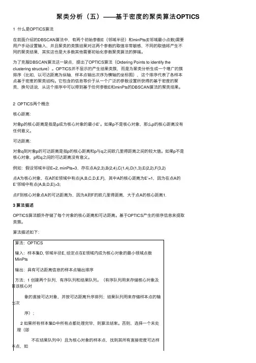
聚类分析(五)——基于密度的聚类算法OPTICS 1 什么是OPTICS算法在前⾯介绍的DBSCAN算法中,有两个初始参数E(邻域半径)和minPts(E邻域最⼩点数)需要⽤户⼿动设置输⼊,并且聚类的类簇结果对这两个参数的取值⾮常敏感,不同的取值将产⽣不同的聚类结果,其实这也是⼤多数其他需要初始化参数聚类算法的弊端。
为了克服DBSCAN算法这⼀缺点,提出了OPTICS算法(Ordering Points to identify theclustering structure)。
OPTICS并不显⽰的产⽣结果类簇,⽽是为聚类分析⽣成⼀个增⼴的簇排序(⽐如,以可达距离为纵轴,样本点输出次序为横轴的坐标图),这个排序代表了各样本点基于密度的聚类结构。
它包含的信息等价于从⼀个⼴泛的参数设置所获得的基于密度的聚类,换句话说,从这个排序中可以得到基于任何参数E和minPts的DBSCAN算法的聚类结果。
2 OPTICS两个概念核⼼距离:对象p的核⼼距离是指是p成为核⼼对象的最⼩E’。
如果p不是核⼼对象,那么p的核⼼距离没有任何意义。
可达距离:对象q到对象p的可达距离是指p的核⼼距离和p与q之间欧⼏⾥得距离之间的较⼤值。
如果p不是核⼼对象,p和q之间的可达距离没有意义。
例如:假设邻域半径E=2, minPts=3,存在点A(2,3),B(2,4),C(1,4),D(1,3),E(2,2),F(3,2)点A为核⼼对象,在A的E领域中有点{A,B,C,D,E,F},其中A的核⼼距离为E’=1,因为在点A的E’邻域中有点{A,B,D,E}>3;点F到核⼼对象点A的可达距离为,因为A到F的欧⼏⾥得距离,⼤于点A的核⼼距离1.3 算法描述OPTICS算法额外存储了每个对象的核⼼距离和可达距离。
基于OPTICS产⽣的排序信息来提取类簇。
算法描述如下:算法:OPTICS输⼊:样本集D, 邻域半径E, 给定点在E领域内成为核⼼对象的最⼩领域点数MinPts输出:具有可达距离信息的样本点输出排序⽅法:1 创建两个队列,有序队列和结果队列。


常⽤聚类算法(基于密度的聚类算法前⾔:基于密度聚类的经典算法 DBSCAN(Density-Based Spatial Clustering of Application with Noise,具有噪声的基于密度的空间聚类应⽤)是⼀种基于⾼密度连接区域的密度聚类算法。
DBSCAN的基本算法流程如下:从任意对象P 开始根据阈值和参数通过⼴度优先搜索提取从P 密度可达的所有对象,得到⼀个聚类。
若P 是核⼼对象,则可以⼀次标记相应对象为当前类并以此为基础进⾏扩展。
得到⼀个完整的聚类后,再选择⼀个新的对象重复上述过程。
若P是边界对象,则将其标记为噪声并舍弃缺陷:如聚类的结果与参数关系较⼤,导致阈值过⼤容易将同⼀聚类分割,或阈值过⼩容易将不同聚类合并固定的阈值参数对于稀疏程度不同的数据不具适应性,导致密度⼩的区域同⼀聚类易被分割,或密度⼤的区域不同聚类易被合并DBSCAN(Density-Based Spatial Clustering of Applications with Noise)⼀个⽐较有代表性的基于密度的聚类算法。
与层次聚类⽅法不同,它将簇定义为密度相连的点的最⼤集合,能够把具有⾜够⾼密度的区域划分为簇,并可在有“噪声”的空间数据库中发现任意形状的聚类。
基于密度的聚类⽅法是以数据集在空间分布上的稠密度为依据进⾏聚类,⽆需预先设定簇的数量,因此特别适合对于未知内容的数据集进⾏聚类。
⽽代表性算法有:DBSCAN,OPTICS。
以DBSCAN算法举例,DBSCAN⽬的是找到密度相连对象的最⼤集合。
1.DBSCAN算法⾸先名词解释:ε(Eps)邻域:以给定对象为圆⼼,半径为ε的邻域为该对象的ε邻域核⼼对象:若ε邻域⾄少包含MinPts个对象,则称该对象为核⼼对象直接密度可达:如果p在q的ε邻域内,⽽q是⼀个核⼼对象,则说对象p从对象q出发是直接密度可达的密度可达:如果存在⼀个对象链p1 , p2 , … , pn , p1=q, pn=p, 对于pi ∈D(1<= i <=n), pi+1 是从 pi 关于ε和MinPts直接密度可达的,则对象p 是从对象q关于ε和MinPts密度可达的密度相连:对象p和q都是从o关于ε和MinPts密度可达的,那么对象p和q是关于ε和MinPts密度相连的噪声: ⼀个基于密度的簇是基于密度可达性的最⼤的密度相连对象的集合。


一种基于密度的空间聚类算法
谱聚类(Spectral Clustering)是一种基于密度的空间聚类算法,旨在根据空间结构,以聚类分隔为几个部分。
这种算法指出,当数据点之间存在一定距离关系时,数据点可以被组织为多个簇,这些簇可以抽象为一个谱,其聚类依赖于谱上的谱级而进行划分。
谱聚类既考虑了空间关系,又考虑了数据的相似性,并将它们有机结合起来。
谱式聚类将数据抽象为一个图模型,模型中的顶点是数据点,边是数据点之间的关系,该图通过计算谱级将结果进行聚类,由此引入基于密度的聚类算法。
谱聚类最常用于聚类紧凑性高的数据集,只有在数据的紧凑性较高的情况下,其聚类结果才能表现出较好的聚类效果。
此外,它还具有反应速度快、聚类结果稳定、聚类结果明确的特点,这是让它被广泛使用的最主要原因,使它成为了当今聚类技术中最重要的算法之一。
基于密度的聚类分割算法
密度聚类分割算法是一种基于密度的聚类算法。
该算法通过计算样本点的密度,并根据样本点周围的密度进行聚类分割。
在该算法中,首先需要确定邻域关系和密度阈值。
然后,根据密度阈值和邻域关系,将样本点分为核心点、边界点和噪声点。
核心点是指其邻域内的样本点数大于等于密度阈值的样本点,边界点是指其邻域内的样本点数小于密度阈值但是与核心点相连的样本点,噪声点是指既不是核心点也不是边界点的样本点。
接着,对核心点进行聚类,将其邻域内的所有样本点都分配到该核心点所在的簇中。
最后,将边界点分配到与其邻域内的核心点所在的簇相同的簇中。
该算法的优点是可以自适应地确定聚类数目,并且能够处理具有任意形状的聚类。
但是,该算法对密度阈值的选取比较敏感,且需要对邻域关系进行预先定义。
- 1 -。
Density-Based Clustering Algorithm DBSCAN,GDBSCAN,OPTICSReporter:An MengyingIntroduction Notion Algorithm PerformanceDBSCANA Density-Based Algorithm forDiscovering Clustersin Large Spatial Databases with NoiseMartin Ester, Hans-Peter Kriegel,Jörg Sander, Xiaowei XuKDD 1996 (pp: 226-231)DBSCAN IntroductionRequirements for Clustering Algorithms:1. Minimal requirements of domain knowledge to determine the input parameters.2. Discovery of clusters with arbitrary shape.3. Good efficiency on large databases.Two basic types of clustering algorithms: partitioning and hierarchical algorithms. Drawbacks of partitioning algorithms(K-means, K-medoids, CLARANS, etc.):1. Local optima2. The number of clusters3. Only convex clustersDrawbacks of hierarchical algorithms(agglomerative approach, divisive approach):1. Termination condition2. Not scale wellMotivation of DBSCAN:Use density to distinguish clusters from noisesKey Idea:For each point of a cluster, the neighborhood of a given radius (Eps) has to contain at least a minimum number of points (MinPts)Definition 1: (Eps-neighborhood of a point) The Eps-neighborhood of a point p, denoted by N Eps (p), is defined N Eps (P) = Definition 2: (directly density-reachable) A point p is directly density-reachable from a point q wrt. Eps, MinPts if1) p ∈ N Eps (q)2) |N Eps (q)| ≥ MinPts (core point condition).Obviously, directly density-reachable is symmetricf or pairs of core points. In general, however, it is not symmetric if one core point and one border point are involved.Eps}.≤ q)dist(p, | D {qDefinition 3: (density-reachable) A point p is density-reachable from a point q wrt. Eps and MinPts if there is a chain of points p l ..... p n, p l = q, p n = p such that p i+1 is directly density-reachable from p i.Definition 4: (density-connected) A point p is density connected to a point q wrt. Eps and MinPtsi f there is a point o such that both, p and q are density-reachable from o wrt. Eps and MinPts.Definition 5: (cluster) Let D be a database of points. A cluster C wrt. Eps and MinPts is a non-empty subset of D satisfying the following conditions:1) if and q is density-reachable from p wrt. Eps and MinPts, then . (Maximality)2) p is density-connectteod q wrt. EPS and MinPts. (Connectivity)Definition 6: (noise) Let C 1 ..... C k be the clusters of the database D wrt. parameters Eps i and MinPts i , i = 1 ..... k. Then we define the noise as the set of points in the database D not belonging to any cluster C i , i.e. noise = }C p :i |C {p i ∉∀∈ :,q p ∀C p ∈C q ∈ :C ,∈∀q pLemma 1: Let p be a point in D and |N Eps (p)| > MinPts. Then the setis a cluster wrt. Eps and MinPts.Lemma 2: Let C be a cluster wrt. Eps and MinPts and let p be any point in C with |N Eps (P)| > MinPts. Then C equals to the set{}MinPts and Eps wrt.p from reachable -density is o and |O D o o ∈={}MinPts and Eps wrt.p from reachable -density is |O o o =DBSCANThe AlgorithmDBSCANHeuristic to determine the parameters Eps and MinPts of the "thinnest" cluster.Let d be the distance of a point p to its k-th nearest neighbor, then the d-neighborhood of p contains exactly k+1 points for almost all points p.Changing k for a point in a cluster does not result in large changes of d.The sorted k-dist graph: sort the points of the database in descending order of their k-dist values.Let a threshold point with the maximal k-dist value in the “thinnest” cluster of D be thedesired parameter value.Often use 4-dist for 2-dimensiona data.MinPts=k=2*dim, Eps=k-dist valueThe precentage of noise is helpful.Determining the Parameters Eps and MinPtsDBSCAN Performance EvaluationDBSCAN Future researchSpatial databases may also contain extended objects such as polygons. We have to develop a definition of the density in an Eps-neighborhood in polygondatabases for generalizing DBSCAN.Second, applications of DBSCAN to high dimensional feature spaces should be investigated. In particular, the shape of the k-dist graph in such applications has to be explored.See the GDBSCANGeneralized Definition SpecializationsApplicationsGDBSCANDensity-Based Clustering in Spatial Databases:The Algorithm GDBSCAN and its ApplicationsJörg Sander, Martin Ester,Hans-Peter Kriegel, Xiaowei Xu1998, 2(2):169-194GDBSCAN - can cluster point objects as well as spatially extended objects according to both their spatial and their non-spatial attributesTwo generalization:First, use any notion of a neighborhood instead of an Eps-neighborhood.Eps → NPred,Second, use other measures to define the “cardinality” of that neighborhood instead of simply counting the objects in a neighborhood of an object .MinPts → MinWeight|N Eps(q)| ≥ MinPts → wCard(S) ≥ MinWeightLemma 3: Let CL be a clustering of D with respect to NPred, MinWeight.If , it holds that p is not a core object, i.e.wCard(NPred(p)) < MinWeight.212121C p all for ,C C and CL ,C C then C ⋂∈≠∈GDBSCAN Important SpecializationsDBSCANThe clustering of spatially extended objects such as polygons.NPred: “intersects” or “meets”,wCard: sum of areas,MinWeight(N): sum of areas ≥ MinAreRegion growingNPred: “neighbor”,MinWeight(N): aggr(non-spatial values) ≥ thresholdGDBSCANApplications1:EarthScience (5D points)2:Molecular Biology (3D points)3:Astronomy (2D points)4:Geography (2D polygons)Motivation Algorithm Density-Based Cluster-Ordering Identifying The Clustering StructureOPTICSOPTICS: Ordering PointsTo Identify the Clustering StructureMihael Ankerst, Markus M. Breunig,Hans-Peter Kriegel, Jörg Sander1999, 28(2):49-60OPTICS MotivationAlmost all clustering algorithms require values forinput parameters which are hard to determineThe algorithms are very sensible to these parameter values, often producing very different partitionings of the data set even for slightly different parametersettings.High-dimensional real-data sets often have a veryskewed distribution that cannot be revealed by aclustering algorithm using only one global parameter setting.For a constant MinPts-value, density-based clusters with respect to a higher density (a lower ε) are completely contained in density-connected sets with respect to a lower density (a higher ε).OPTICS works for an infinite number of distance parameters εi which are smaller than a “generating distance” ε (0 ≤ εi ≤ ε). In this way, the density-based clusters with respect to different densities are constructed simultaneously.We do not assign cluster memberships.Instead, we store the order in which theobjects are processed and the core-distanceand reachability-distance.Definition 5: (core-distance of an object p)Let p be an object from a database D, let ε be a distance value, let Nε (p) be the ε-neighborhood of p, let MinPts be a natural number and let MinPts-distance(p) be the distance from p to its MinPts’neighbor. Then, the core-distance of p is defined as:⎩⎨⎧otherwise),distance(p -MinPts MinPts< (p)) Card(N if ,UNDEFINED = (p)distance -core MinPts ε,Definition 6: (reachability-distance object p w.r.t. object o)Let p and o be objects from a database D, let N ε(o) be the ε-neighborhood of o, and let MinPts be a natural number. Then,the reachability-distance of p with respect to o is defined as:Definition 7: (results of the OPTICS algorithm)Let DB be a database containing n points. The OPTICSalgorithm generates an ordering of the points o:{1...n} →DBand corresponding reachability-values r:{1...n}→ R .⎩⎨⎧otherwisep),,distance(o ),distance(o -max(core MinPts|< (o)) (N | if ,UNDEFINED =o) (p,distance -ty reachabili MinPts ε,The main loopEach object from a database SetOfObjects is simply handed over to a procedure ExpandClusterOrder if the object is not yet processed.Objects which are not yet in the priority-queue OrderSeedsare simply inserted with their reachability-distance.Objects which are already in the queue are moved further tothe top of the queue if their new reachability-distance isThe reachability-plot:It is independent from the dimension of the data set.It is insensitive to the input parameters of the method,i.e. the ε and MinPts.The parameters ε:We can use the expected k-nearest-neighbor distance (for k = MinPts) under the assumption that the objectsare randomly distributed.For a data space DS containing N points. The distance is equal to theradius r of a d-dimensional hypersphere S in DS where S contains exactly k points.The parameters MinPts:The shape of the reachability-plot is very similar for different MinPts. However, lower values → more jaggedhigher values → smoothen and weaken possible “single-link” effects.Our experiments indicate that we will always get good results using values between 10 and 20.Examples:OPTICSIdentifying The Clustering StructureThe attribute-plot:For every point it shows the attribute values (discretized into 256 levels) for every dimension. Underneath each reachability value we plot for each dimension onerectangle in a shade of grey corresponding to the value of this attribute.OPTICS Visualizing Large High-d Data SetsConcepts And Formal Definition Of A Cluster:The reachability value of a point corresponds to the distance of this point to the set of its predecessors.Clusters are dents in the reachability-plot.Clusters in real data sets do not always start and end with extremely steep points.Definition 9: (ξ-steep points)Point p∈{1…n-1} is called a ξ-steep upward point iff it is ξ% lower than its successor:UpPointξ(p) ↔ r(p) ≤ r(p+1) × (1– ξ)Point p∈{1…n-1} is called a ξ-steep downward point iff p’s successor is ξ% lower:DownPointξ(p) ↔ r(p) × (1– ξ) ≥ r(p+1) Definition 10: (ξ-steep areas)Definition 11: (ξ cluster) ReachStart:The first point of D (s D)ReachEnd:The first point after theend of U (e U+1)An Efficient Algorithm To Compute All ξ-ClustersWe start at index=0 with an empty SDASet. While index < n doa)If a new steep down region starts at index, add it to SDASet and continue.b)If a new steep up region starts at index, combine it with every steep downregion in SDASet, check each combination for fulfilling the cluster conditions and save it if it is a cluster. Continue to the right of this steep up region.c)Otherwise, increment index.This is inefficient. So:a)We filter out most potential clusters which will not result in real clusters,b)We get rid of the loop over all points in the cluster.Condition3b is equivalent to:↔OPTICS Experimental Evaluationfigure 20: the runtime of the cluster extractionalgorithm for a data set containing 64-dimensionalcolor histograms extracted from TV-snapshots.figure 22: a reachability-plot for data used in figure 20talk show stork market two TV-stations tennis match different camera anglesimport numpy as npfrom sklearn.cluster import DBSCANfrom sklearn import metricsfrom sklearn.datasets.samples_generator import make_blobsfrom sklearn.preprocessing import StandardScalerfrom pylab import *# Generate sample datacenters = [[1, 1], [-1, -1], [1, -1]]X, labels_true = make_blobs(n_samples=750, centers=centers, cluster_std=0.4, random_state=0) X = StandardScaler().fit_transform(X)sklearn.datasets.make_blobs(n_samples=100, n_features=2, centers=3, cluster_std=1.0, center_box=(-10.0, 10.0), shuffle=True, random_state=None)[source]scatter(xx,yy)show()# save dataf = open("data.txt","w")for i,j in X:f.write(str(i)+","+str(j)+"\n")f.close()# DBSCANdb = DBSCAN(eps=0.3, min_samples=10).fit(X)core_samples = db.core_sample_indices_ # 核心点序号len(core_samples) # 多少个核心点(679个) labels = bels_ # 每个样本点被判为的类别n_clusters_ = len(set(labels)) - (1 if -1 in labels else 0) # 一共几类print n_clusters_ # 3类(不包括噪音点类) num = array([sum(labels==-1),sum(labels==0),sum(labels==1),sum(labels==2)]) print num # array([ 18, 243, 244, 245]) # 每一类中有多少个点CODEds # 聚类结果names(ds) table(ds$isseed) plot(ds, x)ReferencesEster M, Kriegel H P, Sander J, et al. A Density-Based Algorithm for Discovering Clusters in Large Spatial Databases with Noise[J]. 1996.Sander J, Ester M, Kriegel H P, et al. Density-Based Clustering in SpatialDatabases: The Algorithm GDBSCAN and Its Applications[J]. Data Mining and Knowledge Discovery, 1998, 2(2):169-194.Ankerst M, Breunig M M, Kriegel H P, et al. OPTICS: ordering points to identify the clustering structure[J]. Acm Sigmod Record, 1999, 28(2):49-60.。