ALOS 影像的分析与处理
- 格式:pdf
- 大小:1.79 MB
- 文档页数:8
日本ALOS卫星数据图像预处理方法研究-⑴RS应用2010-10-08 15:39:22 阅读107 评论0 字号:大中小订阅引言随着航天遥感技术的发展,多星种、多波段、多分辨率的卫星影像数据不断出现,人们对高分辨率遥感数据的使用,已经有了很大的选择空间。
为了更好的开发利用遥感数据图像信息,提高对多源遥感数据的认知能力,需要对各类遥感图像数据进行处理方法的研究,日本ALOS卫星数据就是其中之一。
关键词:有效灰阶动态度,色强度空间变换模式,线性加权乘积变换模式,乘积变换模式,主分量组分变换模式,三次卷积算法,双线性内插算法,波段同步性,曲向错位。
一.ALOS卫星简介ALOS卫星又称高级陆地观测卫星(Adcanced Land Obsering Satellite,以下简称ALOS),是日本宇航研究开发机构于2006年1月,在日本南部的种子岛航天发射中心(Tanegashima Space Center,NTSC)发射的一颗陆地观测卫星,是日本在1992年发射的地球资源卫星1号和1996年发射的改进型地球观测卫星之后,发射的又一颗自称“更加先进的”陆地观测技术卫星。
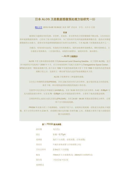
ALOS卫星携带有三种遥感传感器:①全色立体测图传感器(PRISM),具有2.54米的空间几何分辨率,能分别沿轨道方向的前视、垂直下视、和后视快速获取高精度的地面立体信息;②新型可见光和近红外辐射计(AVNIR-2),具有10.00米的空间几何分辨率、0.42~0.69μm可见光谱段波谱分辨率,以及0.76~0.89μm近红外谱段波谱分辨率,主要用于地表面覆盖观测;③相控阵型L-波段合成孔径雷达(PALSAR),具有24.00~89.00米微波谱段极化分辨率,主要用于全天候陆地观测。
PRISM具有独立的三个观测相机,分别用于星下点、前视和后视观测,沿轨道方向获取立体影像,星下点空间分辨率为2.54米。
其观测区域在北纬82°至南纬82°之间,其数据主要用于建立高精度的数字高程模型。

ALOS-1卫星介绍ALOS卫星于2006年1月24日发射,同年2月16日拍摄下第一幅影像。
ALOS卫星载有三个传感器:全色遥感立体测绘仪(PRISM),主要用于数字高程测绘;先进可见光与近红外辐射计-2(AVNIR-2),用于精确陆地观测;相控阵型L波段合成孔径雷达(PALSAR),用于全天时全天候陆地观测。
全色:0.52-0.77 μm蓝色:0.42-0.50μm绿色:0.52-0.60μm红色:0.61-0.69μm近红外:0.76-0.89μmALOS数据产品级别一、PRISM 数据产品Leve1 1A :原始数据分别附带独立的辐射定标和几何定标参数文件。
Leve1 1B1 :对1A数据做辐射校正,增加了绝对定标系数。
Leve1 1B2 :经过辐射与几何校正的产品。
提供地理编码数据和地理参考数据两种选择。
二、AVNIR-2 数据产品Leve1 1A :原始数据附带辐射校正和几何纠正参数。
Leve1 1B1 :对1A数据做辐射校正,增加了绝对定标系数。
Leve1 1B 2:经辐射与几何校正的产品。
提供地理编码数据、地理参考数据和DEM粗纠正数据(限日本区域)三种选择。
三、PALSAR 数据产品Leve1 1.0 :未经处理的原始信号产品,附带辐射与几何纠正参数。
Leve1 1.1 :经过距离向和方位向压缩,斜距产品,单视复数数据。
Leve1 1.5 :经过多视处理及地图投影,未采用DEM高程数据进行几何纠正。
提供地理编码或地理参考数据两种选择,投影方式可选,数据采样间隔根据观测模式可选。
中景视图全色存档数据库中景视图多光谱存档数据库。

第3期,总第77期国 土 资 源 遥 感No .3,2008 2008年9月15日R E M O TE SEN S I N G FO R LAND &R ESOU RC ES Sep.,2008 ALOS 卫星图像分析与预处理实证研究张荣慧,刘顺喜,周连芳,吴海平,何宇华(中国土地勘测规划院土地遥感所,100035 北京)摘要:通过实证研究的方法对高分辨率ALOS 卫星数据进行质量分析,结合ALOS 数据特点,提出了ALOS 原始影像数据的预处理方法和处理流程。
研究结果表明:ALOS 数据预处理工作量较大,且预处理方法要求较为严格,因此,在开展大规模、大范围、大区域、大精度、短周期的图件更新、动态监测等应用时,应考虑将ALOS 卫星图像与其它卫星图像结合使用。
关键词:ALOS 卫星;图像预处理;噪声检测;归一化中图分类号:TP 75 文献标识码:A 文章编号:1001-070X (2008)03-0084-06收稿日期:2007-09-18;修订日期:2008-06-050 引言ALOS 卫星(Advanced Land Observing Satellite )是日本宇航研究开发机构于2006年1月发射的一颗陆地观测卫星,携带有3种遥感传感器:①全色立体测图传感器(PR I S M ),具有2.54m 的空间分辨率,能分别沿轨道方向前视、垂直下视和后视,快速获取高精度的地面立体信息和数字高程模型;②新型可见光和近红外辐射计(AVN I R -2),具有10m的空间分辨率、0.42~0.69μm 可见光谱段波谱分辨率以及0.76~0.89μm 近红外谱段波谱分辨率,主要用于地表面覆盖观测;③相控阵型L 波段合成孔径雷达(P ALS AR ),具有24~89m 微波谱段极化分辨率,主要用于全天候陆地观测。
ALOS 卫星在亚太地区以上行太阳同步轨道方式提供观测数据。
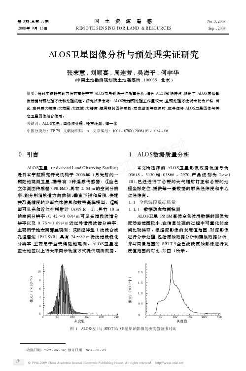
1 ALOS 数据质量分析本文所选择的ALOS 卫星影像数据轨道号为03618-3130和03866-2970,产品级别为Level1B1,已经进行了必要的大气辐射订正和必要的地理坐标定位,提供每一景数据的廓角经纬度和中心点经纬度。

医学影像数据的处理与分析方法随着医学影像技术的迅猛发展,医学影像已经成为临床诊断和治疗过程中不可或缺的一部分。
然而,由于医学影像数据的庞大和复杂性,对其进行处理和分析变得越来越具有挑战性。
本文将探讨一些常用的医学影像处理和分析方法。
一、图像预处理图像预处理是医学影像处理的第一步,旨在消除图像中的噪声和改善图像质量。
其中最常用的方法之一是滤波器的应用。
滤波器可以通过降低图像中的高频噪声来改善图像的视觉效果。
常见的滤波器包括中值滤波器、高斯滤波器等。
二、图像分割图像分割是将医学影像数据划分为不同的区域或结构的过程。
这对于定位和分析特定的组织或病变非常重要。
常见的图像分割方法包括阈值分割、区域生长算法、边缘检测等。
这些方法可以根据图像的像素值、颜色或纹理等特征将图像进行分割。
三、特征提取特征提取是从图像中提取出有用的信息,以描述图像中的结构或病变。
特征提取的目标是减小图像数据的维度,从而方便后续的分析和处理。
常见的特征提取方法包括形态学特征、纹理特征、灰度共生矩阵等。
这些特征可以有效地描述图像的形态、纹理和灰度分布等特征。
四、分类与诊断利用图像处理和分析方法进行分类和诊断是医学影像的重要应用之一。
通过对医学影像数据进行特征提取和分类,可以实现自动化的疾病诊断和预测。
常见的分类方法包括支持向量机、人工神经网络、决策树等。
这些方法可以根据医学影像数据的特征对其进行分类,并帮助医生做出准确的诊断。
五、三维重建与可视化随着医学影像技术的发展,三维重建与可视化成为了医学影像处理中的重要环节。
通过将多个二维图像重建成三维模型,可以提供更加全面和直观的医学信息。
常见的三维重建与可视化方法包括体绘制、表面重建、容积渲染等。
这些方法可以帮助医生更好地理解和分析医学影像数据。
六、前沿技术与挑战除了传统的医学影像处理和分析方法外,一些前沿技术,如深度学习和人工智能,也逐渐应用于医学影像领域。
这些技术可以通过大数据的学习和分析,提高医学影像的自动化和准确性。
北京揽宇方圆信息技术有限公司2014年5月24日JAXA 宇宙航空研究开发机构于种子岛宇宙中心12时5分14秒成功发射了陆地观测技术卫星ALOS-2。
ALOS-2是唯一一个利用L 波段频率的高分辨率星载合成孔径雷达,它能很好的用于监测地壳运动和地球环境,能够不受气候条件和时间的影响获得观测数据。
1-3米的高分辨率,在地球观测卫星上的L 波段合成孔径雷达领域中位居世界第一。
利用如此高的分辨率,ALOS-2卫星能够达到把握灾害状况、农林渔业、海洋观测、资源勘探等多个目的。
在轨参数据或服务描述波束模式分辨率(m)幅宽(km*km)极化方式价格(元)ALOS-2卫星影像聚束(Spotlight)125*25单极化SP 45000超精细(Ultra-Fine)350*70单极化SP /双极化DP 27500高敏感(High-sensitive)650*70单极化SP /双极化DP 27500高敏感(High-sensitive)640*70全极化27500精细(Fine)1070*70单极化SP /双极化DP 27500精细(Fine)1030*70全极化27500(ScanSAR Nominal)标称扫描100(3looks)350*350(5scan)单极化SP /双极化DP 13700扫描宽(ScanSAR Wide)60(1.5looks)490*350(7scan)单极化SP /双极化DP 13700技术能力说明北京揽宇方圆拥有大型正版遥感处理软件,遥感数据处理工程师有10年以上遥感处理工作经验,并有国家大型项目工作经验自主卫星数据处理软件著作权,最大限度保持遥感卫星影像处理的真实度。
公司形象展示信誉证书、荣誉证书、相关资质证书卫星遥感影像技术服务ISO(9001)认证证书复印件高新技术企业认定证明文件国家A级纳税人卫星影像质量快速检验系统著作权登记证历史遥感图像检验系统著作权登记证锁眼卫星影像处理软件著作权登记证多时空多光谱数据处理系统著作权登记证北京揽宇方圆信息技术有限公司。
ALOS-2卫星影像介绍ALOS-2卫星是JAXA的L波段SAR卫星任务ALOS的后继项目,ALOS任务已经于2008年由日本政府批准实施,该任务的总目标是持续提供数据用于绘制地图、区域监视、灾害和环境监测等。
到2010年时,ALOS卫星已经服役了4年(ALOS卫星于2006年发射),这已经完成了该卫星的初始设计寿命目标,并且完成了4项基本目标:绘制地图、区域及灾害监视、资源勘测。
ALOS-2卫星将继承ALOS 卫星的L波段SAR卫星的工作方式,将采用相控阵天线的L波段SAR雷达载荷,扩展数据获取方式,并提升数据品质。
下表显示了ALOS卫星和ALOS-2卫星的性能差别。
表1:ALOS与ALOS-2卫星技术参数对比日本是一个地震多发的国家,这个国家有多座活火山,2/3的国土上覆盖着森林。
这种国土禀赋对L波段SAR雷达的观测具有强烈的选择性。
在此之前发射的两颗卫星上就安装有SAR雷达载荷,分别为在1992~1998年间服役的FUYO-1卫星和在2006~2011年间服役的DAICHI(ALOS)卫星,这些卫星都是用微波进行对地遥感的。
可以直接观测地表面的状况,甚至是直接在夜晚和恶劣天气下工作。
这些雷达遥感卫星最主要的特点就是它们都采用L波段(波长24cm),由于该波段的电磁波具有穿透地表植被层直接获取地面信息的能力。
所以它们对由地震、火山等地壳活动的监测更加准确。
卫星情况:ALOS-2卫星系统由日本三菱电气公司在JAXA指导下开发。
该卫星的性能参数见下表.GPS精确定轨:ALOS-2卫星配备了天基双频GPS接收机,采用L1和L2双波段,用于验证星上自主精密导航技术,可获取更高分辨率的遥感图像并获取高精度轨道摄动模型用于研制下一代地球观测卫星。
JAXA 的导航与控制研究所已经开展了一系列研究用于下一代天基GPS接收机,在这一发展历程中,导航精度的提高是主题。
新的接收机主要在接收多频段和多通道上进行了提高和加强。
北京揽宇方圆信息技术有限公司ALOS-2雷达卫星影像的分析应用日本宇航局从ALOS-2卫星上的相控阵式L波段孔径雷达PALSAR-2获取到了以下影像。
ALOS-2卫星于2014年5月24日发射升空,它获取到的数据将有助于灾难损害监测、森林砍伐监测和海冰观测等。
ALOS-2是利用L波段频率的星载合成孔径雷达卫星,适用于全天候全天时对地球表面进行观测。
以下为ALOS卫星在测试阶段获取到的图像:图1:ALOS-2卫星关东地区影像图1成像于日本时间2014年6月19日上午11时43分,影像采用的观测模式为条带模式,分辨率约为3米。
3米的分辨率是所有安装在对地观测卫星上的L波段合成孔径雷达最优的分辨率,这样高的分辨率将能够更准确的帮助了解地区情况。
图2:ALOS-2及其他卫星东京迪士尼乐园区影像对比图图2为同一区域三颗采用L波段合成孔径雷达的卫星影像对比图,其中左边的图为1992年发射的FUYO-1卫星,中间的图为2006年发射的ALOS卫星。
通过对比可以看出,ALOS-2卫星的分辨率更高。
图3:ALOS-2伊豆大岛区域影像左图为伊豆大岛区域某一个小岛的影像,右图为由ALOS-2上PROSM 传感器所得的高程数据制作而成的鸟瞰图。
图中红色圈圈的区域内呈黑色的部分为2013年10月台风过境引起的大型山体滑坡留下的痕迹。
本图是采用观测到的极化数据制成的假彩色影像,图中绿色代表植被,浅紫色和黄绿色代表城市区域,深紫色代表裸地,这样的影像能够更精确的了解和区分出土地覆盖类型。
图4:ALOS-2和搭载合成孔径雷达的飞机分别拍下的影像右图成像于日本时间2014年6月20日下午10点53分,采用的观测模式为条带式,分辨率约为3米。
左图为搭载了L波段合成孔径雷达的飞机所摄,成像时间为2014年2月4日。
两相对比可以知道,前后相隔约4个月的时间内,由于火山爆发,岛屿面积变大,约增加了0.67平方公里。
右图是在夜间进行观测所得,它也证明了合成孔径雷达可以穿透火山喷发带来的烟雾,因此ALOS-2卫星适用于持续监测火山喷发活动。
GEOMETRIC MODELING AND VALIDATION OF ALOS/PRISM IMAGERY AND PRODUCTSS. Kocaman, A. GruenInstitute of Geodesy and Photogrammetry, ETH Zurich, CH-8092 Zurich, Switzerland (skocaman, agruen)@geod.baug.ethz.chCommission I, WG I/5KEY WORDS: Satellite Remote Sensing, High-resolution Image, Digital Photogrammetry, Calibration, Topographic Mapping, Sensor Orientation, Accuracy AssessmentABSTRACT PRISM is a panchromatic radiometer carried onboard of the new generation Japanese remote sensing satellite ALOS (Advanced Land Observing Satellite). It has three optical systems for forward, nadir and backward views with 2.5 meter spatial resolution. Multiple Linear Array CCD chips are located on the focal plane of each camera, along one across-track line. Three PRISM images per scene are acquired almost simultaneously in forward, nadir and backward viewing angles in along-track direction.The photogrammetric processing of PRISM imagery has special requirements due to the Linear Array CCD sensor structure. As a Member of the ALOS Calibration/Validation Team, we have implemented new algorithms for the geometric processing of the PRISM images, in particular for the interior orientation and self-calibration. In addition, we have refined our physical sensor model according to the multiple optical camera heads of the sensor. Our rigorous model for the PRISM sensor is based on a modified bundle adjustment algorithm with the possibility to use two different trajectory models: the Direct Georeferencing Model with Stochastic Exterior Orientation Elements (DGR) and the Piecewise Polynomial Model (PPM). The given trajectory values are used as stochastic unknowns (observed values) in both approaches in the adjustment. For the self-calibration of the PRISM imagery, we have initially defined 30 additional parameters for the 3 cameras. The parameters are described in accordance with the physical structure of the PRISM imaging sensors. In this paper, PRISM images acquired over three recently generated testfields are used for calibration and geometric validation purposes. We have tested our rigorous sensor model, both with the DGR model and the PPM, using selfcalibration, in all testfields. In addition, we have evaluated the accuracies of the RPCs (Rational Polynomial Coefficients) provided by JAXA/RESTEC in two of the testfields, using three methods: the direct georeferencing (with forward intersection), 2D affine transformation with 6 parameters, and translational correction with 2 shift parameters.PRISM level 1B1 images are used in all tests. The rigorous model produces RMSE values, computed from check points, of about 1/2 pixel in planimetry and 1/3-1/2 pixel in height. Both trajectory models provide sub-pixel accuracy for georeferencing and point positioning in an optimal GCP configuration. However, the PPM requires a higher number of ground control points to obtain stable adjustment results. The direct georeferencing accuracy obtained from the given RPCs is fairly good, and results in 2.5 pixels RMSE in the worst case. The RPC triangulation results show differences between the testfields, requiring different bias-correction terms and GCP distributions for optimal results.1. INTRODUCTION High-resolution satellite images (HRSI) have been widely used in recent years to acquire panchromatic and multispectral images in pushbroom mode for photogrammetric and remote sensing applications. Most of these sensors use Linear Array CCD technology for image sensing and are equipped with high quality orbital position and attitude determination devices like GPS, IMU systems and/or star trackers. The recently launched high resolution satellite sensor ALOS/PRISM is also operating in the pushbroom mode, and has Linear Array CCD pixels with 2.5 meter ground resolution. It provides along-track quasisimultaneous overlapping triplet imagery with three different viewing angles (forward, nadir and backward). For the full exploitation of the potential of the Linear Array CCD sensors’ data, the “classical” satellite image analysis methods must be extended in order to describe the imaging geometry correctly, which is characterized by nearly parallel projection in along-track direction and perspective projection in cross-track direction. In general the processing of this kind of images provides a challenge for algorithmic redesign and opens the possibility to reconsider and improve many photogrammetric processing components. In recent years, some 731amount of research has been devoted to efficiently utilize this high spatial resolution imagery data. Examples for sensor modelling and image orientation can be found in (Baltsavias et al., 2001; Jacobsen, 2003; Grodecki and Dial, 2003; Fraser et al., 2002; Fraser and Hanley, 2003; Gruen and Zhang, 2003; Poli, 2005; Eisenbeiss et al., 2004). We have developed a full suite of new algorithms and the software package SAT-PP (Satellite Image Precision Processing) for the precision processing of HRSI data. The SAT-PP features mainly include: GCP measurements, image georeferencing with RPC approach and various other sensor models, DSM generation with advanced multi-image geometrically constrained Least-Squares matching for Linear Array and single frame sensors, ortho-image generation, feature extraction and others. The software can accommodate images from IKONOS, QuickBird, SPOT5 HRG/HRS, Cartosat-1 and sensors of similar type to be expected in the future. The functionality to accommodate ALOS/PRISM imagery has been added in the context of the work of the ALOS Calibration/Validation Team, organized by JAXA, Japan. Detailed information on the SATPP features can be found in Gruen et al. (2005). The image matcher is described in much detail in Zhang (2005).The International Archives of the Photogrammetry, Remote Sensing and Spatial Information Sciences. Vol. XXXVII. Part B1. Beijing 2008For the georeferencing of aerial Linear Array sensor imagery, a modified bundle adjustment algorithm with the possibility of using three different trajectory models has been developed by Gruen and Zhang (2003). Two of those models, the Direct Georeferencing (DGR) Model with stochastic a priori external orientation constraints and the Piecewise Polynomial Model (PPM) have been modified for the special requirements of the PRISM sensor. Both models have been extended by additional parameters (APs) for self-calibration, to possibly improve the camera’s interior orientation parameters and to model other systematic errors. The APs are defined in accordance with the physical structure of the PRISM cameras. The self-calibration model currently includes nominally a total of 30 APs for all three cameras. Our methods of data processing and previous work on georeferencing of the ALOS/PRISM imagery are published in Gruen et al. (2007) and Kocaman and Gruen (2007a, 2007b). We have recently processed data of three new testfields (Zurich/Winterthur, Switzerland, Wellington, South Africa, and Sakurajima, Japan) and the results are presented in this paper. In addition, the direct geolocation accuracy of the PRISM sensor is assessed using the RPCs of two testfields, Zurich/Winterthur and Sakurajima. The RPCs were generated by JAXA/RESTEC, using their rigorous sensor model. The data was provided by JAXA as a part of ALOS Cal/Val and Science (CVST) Team activities. The position and attitude data are measured by an onboard GPS and startracker. The camera calibration files are generated in the regular calibration process of JAXA. We have evaluated the given RPCs using three methods: the direct georeferencing (with forward intersection), 2D affine transformation with 6 parameters, and translational correction with 2 shift parameters. Different numbers of GCPs are used in the latter two methods. Although the images have particular radiometric problems (Gruen et al., 2007), the sensor orientation results are in general at a good level of accuracy.The calibration data of the PRISM sensor is updated regularly at JAXA EORC. The absolute geolocation accuracies of the three PRISM cameras are given in Table 1.Nadir (RMSE) Forward (RMSE) Backward (RMSE)Pixel direction Line direction Distance (cross-track) (along-track) 6.5 m 7.3 m 9.8 m 8.0 m 14.7 m 16.7 m 7.4 m 16.6 m 18.1 mTable1. PRISM absolute geometric accuracy announced by JAXA EORC (as of 28 September 2007) 2.1 RIGOROUS SENSOR MODELOur rigorous model of the ALOS/PRISM sensor employs modified collinearity equations and uses of two optional trajectory models developed by Gruen and Zhang (2003). The specifications of the PRISM interior and exterior geometries have been taken into account in the models. In the DGR model, the given image trajectory (position and attitude) data are modelled using 9 systematic error correction parameters. In the PPM, the values of the exterior orientation parameters are written as polynomial functions of time. The bundle adjustment solution determines the polynomial coefficients instead of the exterior orientation parameters themselves. Due to the instability of the high-order polynomial models, the piecewise polynomial model is used, in which the full complex trajectory is divided into sections, with each section having its own set of low-order polynomials. Continuity constraints on the orientation parameters at the section boundaries ensure that the calculated positions and attitudes are continuous across the boundaries. The piecewise polynomial model is used to model the position and attitude errors with respect to time. The sensor platform trajectory data, their a priori accuracy values, and sensor relative alignment parameters are provided in the image supplementary files. The attitude and position estimates are based on startracker and GPS receiver data (Iwata, 2003). The sensor alignment parameters are defined in relation to the satellite coordinate system. The knowledge of sensor relative alignment parameters is crucial to transform the platform position and orientation data into the camera coordinate system, which originates at the perspective centre. Although these parameters are provided in the image supplementary files, at the time of this writing, they are not fully employed in our sensor model. The given position values are accurate and used as stochastic unknowns (observed values) in the adjustment. The attitude values are also used as observations, but with smaller weights. Self-calibration is an efficient and powerful technique used for the calibration of photogrammetric imaging systems. The method can use the laboratory calibration data as stochastic input into the adjustment. For the self-calibration of the PRISM imagery, we have initially defined 30 APs in total for the three cameras. The parameters are described in accordance with the physical structure of the PRISM imaging sensors. For more details on the PRISM interior geometry and the APs, please see Gruen et al. (2007) and Kocaman and Gruen (2007a, 2007b). The camera calibration data provided by JAXA are used as input in the adjustment. The calibration data include the focal length values and the relative alignments of the CCD chips. The chip relative alignment values are obtained from in-flight calibration techniques using a large number of GCPs (ca. 7007322. ALOS/PRISM SENSOR MODEL The PRISM sensor features for each viewing angle one particular camera with a number of Linear Array CCD chips in the focal plane. Three PRISM images per scene are acquired almost simultaneously in forward, nadir and backward modes in along-track direction (Figure 1). The nominal viewing angles are (-23.8°, 0°, 23.8).Figure 1. Observation geometry of the ALOS/PRISM triplet mode (Tadono et al., 2004).The International Archives of the Photogrammetry, Remote Sensing and Spatial Information Sciences. Vol. XXXVII. Part B1. Beijing 2008900) and multiple PRISM scenes (ca. 13-15, Tadono et al., 2007). 2.2 Rational Polynomial Functions The Rational Function Models (RFMs) are special forms of polynomial functions. These models do not describe the physical imaging process but use a general polynomial transformation to describe the relationship between image and ground coordinates (Zhang, 2005). The Rational Polynomial Coefficients (RPCs) are often provided by the satellite operator, instead of (e.g. IKONOS) or together with (e.g. Cartosat-1) the rigorous sensor model parameters. When the RPCs are generated from the rigorous sensor models (without use of GCPs), their absolute geolocation accuracies are usually not good enough to meet the requirements of many photogrammetric applications. Grodecki and Dial (2003) proposed a method to blockadjust the high-resolution satellite imagery described by the RFM camera models. With the externally supplied RPCs, the mathematical model used is:x + Δx = x + a0 + a1 x + a 2 y = RPC x (ϕ , λ , h) y + Δy = y + b0 + b1 x + b2 y = RPC y (ϕ , λ , h)The results of four earlier datasets were presented before by Kocaman and Gruen (2007a, 2007b). The results show that the DGR is enough to model the PRISM trajectories. The PPM with larger number of segments causes instabilities and thus a larger number of GCPs are needed to correct for those. Therefore, only one segment per image trajectory has been chosen for the PPM in the tests presented here. The image quality of the PRISM datasets used here is somewhat better than in previous cases. However, there are still some problems, such as jpeg compression artifacts, which cause problems in GCP image definition/measurement and in matching. The given attitude values of the Zurich/Winterthur dataset were extracted and transformed precisely from the ECI (Earth Centered Inertial) coordinate system into the ECR (Earth Centered Rotating) coordinate system. However, due to partially missing sensor relative alignment values in the transformation, corrections in form of three attitude shift parameters per camera needed to be estimated in the adjustment. The a priori standard deviations used for the attitude shift and drift parameters in the tests were 0.07° per image and 6.25°×106 per 1000 lines, respectively. These values were computed from the results of previous adjustments of the Zurich/Winterthur dataset with all GCPs. The a priori standard deviations of the trajectory position values were the same for all datasets and 2 m in all three directions. The a priori standard deviations of the image measurements were assumed to be half a pixel. The RPCs were evaluated in two testfields (Zurich/Winterthur and Sakurajima) with three different methods (DG, RPC-2, RPC-6). The results are presented in the following sections. 3.1 Zurich/Winterthur Testfield, Switzerland The Zurich/Winterthur testfield has been established by the IGP, ETH Zurich in summer 2007 under an ESA-ESRIN contract. The PRISM image triplet has been acquired on 22 April 2007. During the GPS measurement campaign, the images were used to select the control points. A total of 99 GCPs were measured in the field and also in the PRISM images. In addition, 101 tie points were measured on the images. The point distribution in the PRISM nadir image is represented in Figure 2. In the rigorous model, we used 1, 2, 4, and 9 GCP configurations with homogeneous distributions in planimetry. The a posteriori sigma naught values are equal to 0.3 pixels for all tests. When only 1 GCP is used, the RMSE values are equal to 1.3 and 3 pixels in planimetry and height, respectively. Already with only 2 GCPs, a sub-pixel accuracy level could be achieved with the DGR method (Figure 3). The PPM has been tested only in the 9 GCP configuration. Comparing the 2, 4, and 9 GCP configurations we find that the planimetric accuracy is slightly worse in the 2 GCPs case compared to the other cases, while the height accuracy remains almost the same in all cases. The accuracy both in planimetry and height, as evidenced by RMSE(XY) and RMSE(Z), is below one pixel in all tests. The PPM results are the same as the DGR model results of the same 9 GCP configuration.(1)Where, a0, a1, a2 and b0, b1, b2 are the parameters of a 2D affine transformation for each image, and (x,y) and (ϕ,λ,h) are image and object coordinates of the points. We have the possibility to post-correct given RPCs in SAT-PP using two different methods: RPC-2: Two shift parameters (a0,b0 of Eq. 1) are applied to correct the RPCs RPC-6: The full 2D affine transformation (Eq. 1) with 6 parameters is applied In both cases we need a certain number of GCPs (at least one in the first and three in the second case) in order to determine the parameters. We have evaluated the accuracies of the Zurich/Winterthur and Sakurajima RPCs provided by JAXA/RESTEC using these methods. In addition, we have performed a direct georeferencing (DG) test by computing the ground coordinates of each GCP using the given RPCs in a forward intersection with multiple rays procedure. Object space residuals, which are obtained from the comparison of computed coordinates with the given ones, are analyzed with statistical methods and also by visual checks.3. EMPIRICAL TESTS We have processed data over three testfields: Zurich/Winterthur, Switzerland, Sakurajima, Japan, and Wellington, South Africa. The DGR model has been tested in all testfields. The PPM with one segment and the RFM approach have been only applied to the Zurich/Winterthur and Sakurajima datasets. The empirical tests given in the following sections employ self-calibration with 2 APs per image, which are the scale parameter and the CCD line bending parameter (6 APs in total). For the accuracy assessment the RMSE values, which are computed from the differences between the given and the estimated coordinates of the check points, and the standard deviations, computed from the covariance matrix of unknowns, were used. 733The International Archives of the Photogrammetry, Remote Sensing and Spatial Information Sciences. Vol. XXXVII. Part B1. Beijing 2008Figure 2. Point distribution in the Zurich/Winterthur testfield. The red circles represent the GCP locations.Figure 4. Object space residuals in the Zurich/Winterthur testfield obtained from the DG with the given RPCs. The given RPCs were corrected using the RPC-2 and RPC-6 methods (Table 3) with three different GCP configurations. The three corner points depicted with triangles in Figure 4 were used as control points in the 3 GCP case. As can be seen from Table 3, the georeferencing accuracy was not improved in this case. Also, the systematic effects could not be removed from the residuals by this procedure. σ0 (pixel) 0.63 0.73 0.41 0.51 0.39 0.49Model RPC-6 RPC-2 RPC-6 RPC-2 RPC-6 RPC-2GCP RMSE(XY)(m) RMSE(Z)(m) All 1.3 2.3 All 1.5 2.5 6 1.4 2.4 6 1.6 2.5 3 1.4 3.3 3 1.6 3.9Table 3. RPC correction results in the Zurich/Winterthur testfield Figure 3. Accuracy results of the Zurich/Winterthur tests with rigorous sensor models Considering the self-calibration, four of the additional parameters (scale parameters of the forward-nadir-backward images and the CCD line bending parameter of the nadir image) were statistically significant in the Zurich/Winterthur tests. The DG accuracy values obtained from the RPCs provided by JAXA/RESTEC are presented in Table 2. The results are at subpixel level in planimetry and one pixel in height. There are local systematic effects in the residuals (Figure 4). 3.2 Sakurajima Testfield, Japan The Sakurajima testfield was generated as a joint project of Kochi Institute of Technology and Kanazawa Institute of Technology. 31 GCPs, provided by the Japan Association of Remote Sensing (JARS), have a rather uneven distribution, caused in parts by the special topography (Figure 5). The PRISM image triplet was acquired on 8 November 2006. 60 tie points were measured on the images using semi-automated matching. The rigorous model was tested using the DGR and the PPM with a single segment per image. The tests were performed using different numbers of GCPs and the results are provided in Figure 6. The DG results in this testfield are presented in Table 4 and Figure 7. The systematic errors in the residuals could be removed using GCPs in the RPC correction adjustment (Table 5).RMSE Mean Max. residualX (m) 1.7 0.6 4.0Y (m) 1.7 0.9 4.2Z (m) 2.5 -0.1 5.6Table 2. DG accuracy values obtained from the RPCs provided by JAXA/RESTEC for the Zurich/Winterthur testfield734The International Archives of the Photogrammetry, Remote Sensing and Spatial Information Sciences. Vol. XXXVII. Part B1. Beijing 200867 ground control and 32 tie points were used in the triangulation tests (Figure 8). The GCPs were pre-selected on the PRISM images and surveyed by the Dept. of Architecture, Planning and Geomatics, University of Cape Town in September 2007. The averaged standard deviations of the GPS measurements are 3 cm in planimetry and height. GCP RMSE(XY)(m) RMSE(Z)(m) σ0 (pixel) All 1.3 1.1 0.58 All 1.4 2.0 0.68 6 1.4 1.4 0.39 6 1.5 2.1 0.56 3 1.8 1.4 0.37 3 1.8 3.4 0.51Model RPC-6 RPC-2 RPC-6 RPC-2 RPC-6 RPC-2Table 5. RPC correction accuracy results for the Sakurajima testfieldFigure 5. Overview of the GCP distribution in the PRISM nadir image of Sakurajima. The red circles represent the GCPs.Figure 7. Object space residuals in the Sakurajima testfield obtained from the DG with the given RPCs.Figure 6. Rigorous sensor model results in the Sakurajima testfield X (m) 1.6 1.1 4.0 Y (m) 4.9 -4.6 7.6 Z (m) 6.4 -6.1 12.1RMSE Mean Max. residual (absolute)Table 4. DG accuracy values obtained from the RPCs provided by JAXA/RESTEC for the Sakurajima testfield 3.1 Wellington Testfield, South Africa The Wellington testfield is located in the north-east of Cape Town, South Africa, in an area not so much affected by the clouds and occasional fog of Cape Town. The PRISM images over the Wellington testfield were acquired on 19 April 2007. The images were tested with the DGR model with selfcalibration, using different subsets of GCPs. 735Figure 8. Overview of the control and tie point distribution on the PRISM nadir image. The red circles represent the GCP locations.The International Archives of the Photogrammetry, Remote Sensing and Spatial Information Sciences. Vol. XXXVII. Part B1. Beijing 2008The results from the DGR model computations are presented in Figure 9. 4 GCPs are enough to reach the accuracy potential in planimetry. However, in height, there is still some improvement visible when going from 4 to 6 GCPs.functions have not yet been fully explored for PRISM imagery. In any case, self-calibration should be used with great care and not blindly. The statistical testing of additional parameters for determinability is a crucial requirement for a successful use of this technique. If we compare these georeferencing results with those which were obtained earlier with other satellite sensors of similar type (SPOT-5, IKONOS, QuickBird) we note that the accuracy (expressed in pixels) is about the same as with these other sensors.3.00 2.50 2.001.50 1.00mREFERENCES0.50 0.00 2 1.84 1.34 1.00 2.80 0.45 3 1.83 1.41 0.96 2.71 0.45 4 1.55 1.44 0.90 2.55 0.46 5 1.53 1.29 0.89 2.53 0.46 6 1.50 1.21 0.88 2.48 0.46 9 1.52 1.21 0.86 2.43 0.47GCP noRMSE(XY) RMSE(Z) Sigma(XY) Sigma(Z) Sigma0 (pixels)Baltsavias E. P., Pateraki M., Zhang L., 2001. Radiometric and Geometric Evaluation of IKONOS Geo Images and Their Use for 3D Building Modeling. In Proceedings of Joint ISPRS Workshop on "High Resolution Mapping from Space 2001", 19-21 September, Hannover, Germany (on CD-ROM). Eisenbeiss H., Baltsavias E. P., Pateraki M., Zhang L., 2004. Potential of IKONOS and QUICKBIRD Imagery for Accurate 3D-Point Positioning, Orthoimage and DSM Generation. International Archives of Photogrammetry, Remote Sensing and Spatial Information Sciences, 35 (B3), pp. 522-528. Fraser C., Baltsavias E. P., Gruen A., 2002. Processing of IKONOS Imagery for Sub-meter 3D Positioning and Building Extraction. ISPRS Journal of Photogrammetry & Remote Sensing, 56(3), pp. 177-194. Fraser C., Hanley H. B., 2003. Bias Compensation in Rational Functions for IKONOS Satellite Imagery. Photogrammetric Engineering and Remote Sensing, 69(1), pp. 53-57. Grodecki J., Dial G., 2003. Block Adjustment of HighResolution Satellite Images Described by Rational Polynomials. Photogrammetric Engineering and Remote Sensing, 69(1), pp. 59-68. Gruen A., Zhang L., 2003. Sensor Modeling for Aerial Triangulation with Three-Line-Scanner (TLS) Imagery. Journal of Photogrammetrie, Fernerkundung, Geoinformation (PFG), 2/2003, pp. 85-98. Gruen A., Zhang L., Eisenbeiss H., 2005. 3D Precision Processing Of High Resolution Satellite Imagery. ASPRS 2005, Baltimore, Maryland, USA, March 7-11 (on CD-ROM). Gruen A., Kocaman S., Wolff K., 2007. Calibration and Validation of Early ALOS/PRISM Images. The Journal of the Japan Society of Photogrammetry and Remote Sensing, Vol 46, No. 1, pp. 24-38. Iwata T., 2003. Precision Geolocation Determination and Pointing Management for the Advanced Land Observing Satellite (ALOS). IEEE/IGARSS 2003, Toulouse, France, July 21-25. Jacobsen K., 2003. Geometric Potential of IKONOS and QuickBird-Images. Photogrammetric Week ’03, Ed. D. Fritsch, pp. 101-110. JAXA EORC, 2007. PRISM absolute geolocation accuracies. http://www.eorc.jaxa.jp/hatoyama/satellite/data_tekyo_setsumei /alos_hyouka_e.html. Last accessed on 29.04.2008. 736Figure 9. DGR model results in the Wellington testfield4. CONCLUSIONS We have calibrated and validated ALOS/PRISM images over three testfields: Zurich/Winterthur, Switzerland, Sakurajima, Japan and Wellington, South Africa. For georeferencing we applied both our sensor/trajectory models DGR and PPM and found that DGR had the better performance in case of very few GCPs. In case of the Zurich/Winterthur and Sakurajima datasets, with correct a priori definition of the interior and exterior orientation elements, 2 GCPs were enough to achieve sub-pixel accuracy. Concerning the planimetric accuracy the theoretical expectations Sigma(XY) were usually significantly better than the empirical values RMSE(XY). However, we note that in many cases the empirical height accuracy values RMSE(Z) were even better than the corresponding theoretical precision values. This somewhat inconsistent behavior results from the fact that the height-related definition of the GCPs and check points in image space is better than the planimetric one. Over all three testfields we achieved with our sensor model DGR quite consistent accuracy results. We stay in all cases in the sub-pixel domain, in the best cases we achieved about half a pixel planimetric accuracy and 1/3 pixel height accuracy. This relatively high accuracy is surprising, considering the fact that the image quality of PRISM has still much potential for improvement. On the other side one usually uses only well defined points as GCPs and check points, where the inferior image quality has not such a negative influence. When using the supplied RPCs we achieved accuracies between 0.7 and 2.6 pixels. In these cases we noticed systematic effects in the check point residuals, which could partially be removed when using RPC correction terms together with GCPs. This also improved the georeferencing accuracy in parts quite substantially (up to a factor 4.6 in height). Yet, we do not have sufficiently broad experiences with the use of supplied RPCs. Their quality depends on the local navigation values. To be on the save side it is still advisable to use a few GCPs for RPC correction. Self-calibration is a very powerful method for sensor model refinement. However, the most appropriate additional parameterThe International Archives of the Photogrammetry, Remote Sensing and Spatial Information Sciences. Vol. XXXVII. Part B1. Beijing 2008Kocaman S., Gruen A., 2007a. Orientation and Calibration of ALOS/PRISM Imagery. International Archives of Photogrammetry, Remote Sensing and Spatial Information Sciences, Vol. XXXVI, Part I/W51, Proceedings of ISPRS Hannover Workshop 2007 (on CD-ROM). Kocaman S., Gruen A., 2007b. Rigorous Sensor Modeling of ALOS/PRISM Imagery. Proceedings of the 8th Conference on “Optical 3D Measurement Techniques”, Zurich, Switzerland, 912 July, Vol. I, pp. 204-213. Poli D., 2005. Modelling of Spaceborne Linear Array Sensors. Ph. D. Dissertation, IGP Report No. 85, ISSN 0252-9335 ISBN 3-906467-3, Institute of Geodesy and Photogrammetry, ETH Zurich, Switzerland, 204 pages. Tadono T., Shimada M., Watanabe M., Hashimoto T., Iwata T., 2004. Calibration and Validation of PRISM Onboard ALOS. International Archives of Photogrammetry, Remote Sensing and Spatial Information Sciences, Vol.XXXV part B1, pp. 13-18. Tadono T., Shimada M., Iwata T., Takaku J., 2007. Accuracy assessment of geolocation determination for PRISM and AVNIR-2 onboard ALOS. Proceedings of the 8th Conference on “Optical 3D Measurement Techniques”, Zurich, Switzerland, 9-12 July, Vol. I, pp. 214-222. Zhang, L., 2005. Automatic Digital Surface Model (DSM) Generation from Linear Array Images. Ph.D. Dissertation, No. 88, Institute of Geodesy and Photogrammetry, ETH Zurich, Switzerland.Acknowledgements The authors would like to thank JAXA and RESTEC, Japan, ESA/ESRIN, Italy, and GAEL, France for supporting us in the acquisition of the reference data and for their continuous support throughout this study. Special thanks go to some members of the Chair of Photogrammetry and Remote Sensing, ETH Zurich for their valuable support in the preparation of the Zurich/Winterthur testfield and to Prof. Heinz Ruether for the organization of the GPS measurements in the Wellington testfield.737。