计算方法龙格库塔方法概要

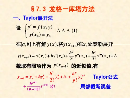
数值分析中，龙格－库塔法（Runge-Kutta）是用于模拟常微分方程的解的重要的一类隐式或显式迭代法。

这些技术由数学家卡尔·龙格和马丁·威尔海姆·库塔于1900年左右发明。

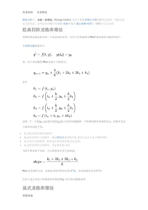
经典四阶龙格库塔法龙格库塔法的家族中的一个成员如此常用，以至于经常被称为“RK4”或者就是“龙格库塔法”。

令初值问题表述如下。

则，对于该问题的RK4由如下方程给出：其中这样，下一个值(y n+1)由现在的值(y n)加上时间间隔(h)和一个估算的斜率的乘积决定。

该斜率是以下斜率的加权平均：∙k1是时间段开始时的斜率；∙k2是时间段中点的斜率，通过欧拉法采用斜率k1来决定y在点t n + h/2的值；∙k3也是中点的斜率，但是这次采用斜率k2决定y值；∙k4是时间段终点的斜率，其y值用k3决定。

当四个斜率取平均时，中点的斜率有更大的权值：RK4法是四阶方法，也就是说每步的误差是h5阶，而总积累误差为h4阶。

注意上述公式对于标量或者向量函数(y可以是向量)都适用。

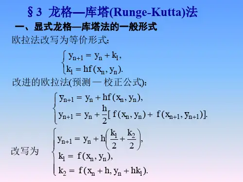
显式龙格库塔法显示龙格－库塔法是上述RK4法的一个推广。

它由下式给出其中如果要求方法有精度p则还有相应的条件，也就是要求舍入误差为O(h p+1)时的条件。

这些可以从舍入误差本身的定义中导出。

例如，一个2阶精度的2段方法要求b1 + b2 = 1, b2c2 = 1/2, 以及b2a21 = 1/2。

在Matlab下输入：edit，然后将下面两行百分号之间的内容，复制进去，保存%%%%%%%%%%%%%%%%%%%%%%%%%%%%%%%%%%%%%% %%%%%%%%%%%%%%%%%%%%%%%%%%%%%function dxdt=ode_Miss_ghost(t,x)%分别用x(1),x(2),x(3),x(4)代替N1,P1,N2,P2N1=x(1);P1=x(2);N2=x(3);P2=x(4);K=2;tau_c=3e-9;tan_p=6e-12;beta =5e-5;delta=0.692;eta =0.0001;fm =8e6;Ith =26e-3;Ib =1.5*Ith;Im =0.3*Ith;I1=Ib+Im*sin(2*pi*fm*t)+K*P2;I2=Ib+Im*sin(2*pi*fm*t)+K*P1;dxdt=[(I1/Ith-N1-(N1-delta)/(1-delta)*P1)/tau_e;((N1-delta)/(1-delta)*(1-eta*P1)*P1-P1+beta*N1)/tau_p;(I2/Ith-N2-(N2-delta)/(1-delta)*P2)/tau_e;((N2-delta)/(1-delta)*(1-eta*P2)*P2-P2+beta*N2)/tau_p;]; %%%%%%%%%%%%%%%%%%%%%%%%%%%%%%%%%%%%%% %%%%%%%%%%%%%%%%%%%%%%%%%%%%%%在Matlab下面输入：t_start=0;t_end=2e-9;y0=[1e-3;1e-4;0;0]; %初值[x,y]=ode15s('ode_Miss_ghost',[0,t_end],y0);plot(x,y);legend('N1','P1','N2','P2');xlabel('x');Mathlab定步长龙格－库塔法[345阶]、自适应步长rkf45经常看到很多朋友问定步长的龙格库塔法设置问题，下面吧定步长三阶、四阶、五阶龙格库塔程序贴出来，有需要的可以看看ODE3 三阶龙格－库塔法CODE:function Y = ode3(odefun,tspan,y0,varargin)%ODE3 Solve differential equations with a non-adaptive method of order 3.% Y = ODE3(ODEFUN,TSPAN,Y0) with TSPAN = [T1, T2, T3, ... TN] integrates% the system of differential equations y' = f(t,y) by stepping from T0 to% T1 to TN. Function ODEFUN(T,Y) must return f(t,y) in a column vector.% The vector Y0 is the initial conditions at T0. Each row in the solution% array Y corresponds to a time specified in TSPAN.%% Y = ODE3(ODEFUN,TSPAN,Y0,P1,P2...) passes the additional parameters% P1,P2... to the derivative function as ODEFUN(T,Y,P1,P2...).%% This is a non-adaptive solver. The step sequence is determined by TSPAN% but the derivative function ODEFUN is evaluated multiple times per step.% The solver implements the Bogacki-Shampine Runge-Kutta method of order 3.%% Example% tspan = 0:0.1:20;% y = ode3(@vdp1,tspan,[2 0]);% plot(tspan,y(:,1));% solves the system y' = vdp1(t,y) with a constant step size of 0.1, % and plots the first component of the solution.%if ~isnumeric(tspan)error('TSPAN should be a vector of integration steps.');endif ~isnumeric(y0)error('Y0 should be a vector of initial conditions.');endh = diff(tspan);if any(sign(h(1))*h <= 0)error('Entries of TSPAN are not in order.')endtryf0 = feval(odefun,tspan(1),y0,varargin{:});catchmsg = ['Unable to evaluate the ODEFUN at t0,y0. ',lasterr];error(msg);endy0 = y0(:); % Make a column vector.if ~isequal(size(y0),size(f0))error('Inconsistent sizes of Y0 and f(t0,y0).');endneq = length(y0);N = length(tspan);Y = zeros(neq,N);F = zeros(neq,3);Y(:,1) = y0;for i = 2:Nti = tspan(i-1);hi = h(i-1);yi = Y(:,i-1);F(:,1) = feval(odefun,ti,yi,varargin{:});F(:,2) = feval(odefun,ti+0.5*hi,yi+0.5*hi*F(:,1),varargin{:});F(:,3) = feval(odefun,ti+0.75*hi,yi+0.75*hi*F(:,2),varargin{:});Y(:,i) = yi + (hi/9)*(2*F(:,1) + 3*F(:,2) + 4*F(:,3));endY = Y.';ODE4 四阶龙格－库塔法CODE:function Y = ode4(odefun,tspan,y0,varargin)%ODE4 Solve differential equations with a non-adaptive method of order 4.% Y = ODE4(ODEFUN,TSPAN,Y0) with TSPAN = [T1, T2, T3, ... TN] integrates % the system of differential equations y' = f(t,y) by stepping from T0 to% T1 to TN. Function ODEFUN(T,Y) must return f(t,y) in a column vector.% The vector Y0 is the initial conditions at T0. Each row in the solution% array Y corresponds to a time specified in TSPAN.%% Y = ODE4(ODEFUN,TSPAN,Y0,P1,P2...) passes the additional parameters % P1,P2... to the derivative function as ODEFUN(T,Y,P1,P2...).%% This is a non-adaptive solver. The step sequence is determined by TSPAN % but the derivative function ODEFUN is evaluated multiple times per step.% The solver implements the classical Runge-Kutta method of order 4.%% Example% tspan = 0:0.1:20;% y = ode4(@vdp1,tspan,[2 0]);% plot(tspan,y(:,1));% solves the system y' = vdp1(t,y) with a constant step size of 0.1,% and plots the first component of the solution.%if ~isnumeric(tspan)error('TSPAN should be a vector of integration steps.');endif ~isnumeric(y0)error('Y0 should be a vector of initial conditions.');endh = diff(tspan);if any(sign(h(1))*h <= 0)error('Entries of TSPAN are not in order.')endtryf0 = feval(odefun,tspan(1),y0,varargin{:});catchmsg = ['Unable to evaluate the ODEFUN at t0,y0. ',lasterr]; error(msg);endy0 = y0(:); % Make a column vector.if ~isequal(size(y0),size(f0))error('Inconsistent sizes of Y0 and f(t0,y0).');endneq = length(y0);N = length(tspan);Y = zeros(neq,N);F = zeros(neq,4);Y(:,1) = y0;for i = 2:Nti = tspan(i-1);hi = h(i-1);yi = Y(:,i-1);F(:,1) = feval(odefun,ti,yi,varargin{:});F(:,2) = feval(odefun,ti+0.5*hi,yi+0.5*hi*F(:,1),varargin{:}); F(:,3) = feval(odefun,ti+0.5*hi,yi+0.5*hi*F(:,2),varargin{:}); F(:,4) = feval(odefun,tspan(i),yi+hi*F(:,3),varargin{:});Y(:,i) = yi + (hi/6)*(F(:,1) + 2*F(:,2) + 2*F(:,3) + F(:,4));endY = Y.';定步长RK4(自编):CODE:function Y=RungeKutta4(f,xn,y0)% xn=0:.1:1;% y0=1;% y_n=[];% f=@(X1,Y1) Y1-2*X1/Y1;y_n=[];h=diff(xn(1:2));for i=1:length(xn)-1K1=f(xn(i),y0);K2=f(xn(i)+h/2,y0+h*K1/2);K3=f(xn(i)+h/2,y0+h*K2/2);K4=f(xn(i)+h,y0+h*K3);y_n=[y_n;y0+h/6*(K1+2*K2+2*K3+K4)];y0=y_n(end);endY=y_n;ODE5 五阶龙格－库塔法CODE:function Y = ode5(odefun,tspan,y0,varargin)%ODE5 Solve differential equations with a non-adaptive method of order 5.% Y = ODE5(ODEFUN,TSPAN,Y0) with TSPAN = [T1, T2, T3, ... TN] integrates % the system of differential equations y' = f(t,y) by stepping from T0 to% T1 to TN. Function ODEFUN(T,Y) must return f(t,y) in a column vector.% The vector Y0 is the initial conditions at T0. Each row in the solution% array Y corresponds to a time specified in TSPAN.%% Y = ODE5(ODEFUN,TSPAN,Y0,P1,P2...) passes the additional parameters % P1,P2... to the derivative function as ODEFUN(T,Y,P1,P2...).%% This is a non-adaptive solver. The step sequence is determined by TSPAN % but the derivative function ODEFUN is evaluated multiple times per step.% The solver implements the Dormand-Prince method of order 5 in a general % framework of explicit Runge-Kutta methods.%% Example% tspan = 0:0.1:20;% y = ode5(@vdp1,tspan,[2 0]);% plot(tspan,y(:,1));% solves the system y' = vdp1(t,y) with a constant step size of 0.1,% and plots the first component of the solution.if ~isnumeric(tspan)error('TSPAN should be a vector of integration steps.');endif ~isnumeric(y0)error('Y0 should be a vector of initial conditions.');endh = diff(tspan);if any(sign(h(1))*h <= 0)error('Entries of TSPAN are not in order.')endtryf0 = feval(odefun,tspan(1),y0,varargin{:});catchmsg = ['Unable to evaluate the ODEFUN at t0,y0. ',lasterr];error(msg);endy0 = y0(:); % Make a column vector.if ~isequal(size(y0),size(f0))error('Inconsistent sizes of Y0 and f(t0,y0).');endneq = length(y0);N = length(tspan);Y = zeros(neq,N);% Method coefficients -- Butcher's tableau%% C | A% --+---% | BC = [1/5; 3/10; 4/5; 8/9; 1];A = [ 1/5, 0, 0, 0, 03/40, 9/40, 0, 0, 044/45 -56/15, 32/9, 0, 019372/6561, -25360/2187, 64448/6561, -212/729, 0 9017/3168, -355/33, 46732/5247, 49/176, -5103/18656];B = [35/384, 0, 500/1113, 125/192, -2187/6784, 11/84]; % More convenient storageA = A.';B = B(:);nstages = length(B);F = zeros(neq,nstages);Y(:,1) = y0;for i = 2:Nti = tspan(i-1);hi = h(i-1);yi = Y(:,i-1);% General explicit Runge-Kutta frameworkF(:,1) = feval(odefun,ti,yi,varargin{:});for stage = 2:nstageststage = ti + C(stage-1)*hi;ystage = yi + F(:,1:stage-1)*(hi*A(1:stage-1,stage-1));F(:,stage) = feval(odefun,tstage,ystage,varargin{:});endY(:,i) = yi + F*(hi*B);endY = Y.';-------------------------------------------------------------------------------------------------------------------自适应步长RKF45(相当于ode45)ODE45 是4阶方法提供候选解，5阶方法控制误差。

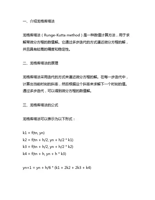
一、介绍龙格库塔法龙格库塔法（Runge-Kutta method）是一种数值计算方法，用于求解常微分方程的数值解。

它通过多步迭代的方式逼近微分方程的解，并且具有较高的精度和稳定性。

二、龙格库塔法的原理龙格库塔法采用迭代的方式来逼近微分方程的解。

在每一步迭代中，计算出当前时刻的斜率，然后根据这个斜率来求解下一个时刻的值。

通过多步迭代，可以得到微分方程的数值解。

三、龙格库塔法的公式龙格库塔法可以表示为以下形式：k1 = f(tn, yn)k2 = f(tn + h/2, yn + h/2 * k1)k3 = f(tn + h/2, yn + h/2 * k2)k4 = f(tn + h, yn + h * k3)yn+1 = yn + h/6 * (k1 + 2k2 + 2k3 + k4)其中，k1、k2、k3、k4为斜率，h为步长，tn为当前时刻，yn为当前时刻的解，yn+1为下一个时刻的解。

四、使用matlab实现龙格库塔法在MATLAB中，可以通过编写函数来实现龙格库塔法。

下面是一个用MATLAB实现龙格库塔法的简单例子：```matlabfunction [t, y] = runge_kutta(f, tspan, y0, h)t0 = tspan(1);tf = tspan(2);t = t0:h:tf;n = length(t);y = zeros(1, n);y(1) = y0;for i = 1:n-1k1 = f(t(i), y(i));k2 = f(t(i) + h/2, y(i) + h/2 * k1);k3 = f(t(i) + h/2, y(i) + h/2 * k2);k4 = f(t(i) + h, y(i) + h * k3);y(i+1) = y(i) + h/6 * (k1 + 2*k2 + 2*k3 + k4);endend```以上就是一个简单的MATLAB函数，可以利用该函数求解给定的微分方程。

《四阶龙格—库塔法的原理及其应用》
龙格—库塔法(又称龙格库塔法)是由一系列有限的、独立的可能解组成的无穷序列,这些解中每个都与原来的数列相差一个常数。

它是20世纪30年代由匈牙利著名数学家龙格和库塔提出的,故得此名。

1.它的基本思想是:在n 阶方阵M 上定义一个函数,使得当n 趋于无穷时,它在m 中所表示的数值为M 的某种特征值,从而构造出一族具有某种特性的可计算函数f (x)= Mx+ C (其中C 为任意正整数)。

例如,若f (x)=(a-1) x+ C,则称之为(a-1) x 的龙格—库塔法。

2.它的应用很广泛,可以求解各类问题,且能将大量的未知数变换成少数几个已知数,因此它是近似计算的一种重要工具。

3.
它的优点主要有:(1)可以将多项式或不等式化成比较简单的形式;(2)对于同一问题可以用不同的方法来解决,并取得同样的结果;(3)适合处理高次多项式或者不等式,尤其适合处理多元函数的二次型。

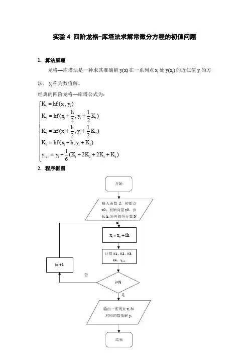
四阶龙格－库塔法求解常微分方程的初值问题1.算法原理对于一阶常微分方程组的初值问题⎪⎪⎪⎩⎪⎪⎪⎨⎧=⋯⋯==⋯⋯=⋯⋯⋯⋯=⋯⋯=0020********'212'2211'1)(,,)(,)())(,),(),(,()())(,),(),(,()())(,),(),(,()(n n n n n n n y x y y x y y x y x y x y x y x f x y x y x y x y x f x y x y x y x y x f x y ， 其中b x a ≤≤。

若记Tn Tn Tn y x f y x f y x f y x f y y y y x y x y x y y x y )),(,),,(),,((),(),,,())(),(),(()(2102010021⋯⋯=⋯⋯=⋯⋯=，，则可将微分方程组写成向量形式⎩⎨⎧=≤≤=0')()),(,()(y a y b x a x y x f x y微分方程组初值问题在形式上和单个微分方程处置问题完全相同，只是数量函数在此变成了向量函数。

因此建立的单个一阶微分方程初值问题的数值解法，可以完全平移到求解一阶微分方程组的初值问题中，只不过是将单个方程中的函数转向向量函数即可。

标准4阶R-K 法的向量形式如下：⎪⎪⎪⎪⎩⎪⎪⎪⎪⎨⎧++=++=++==++++=+),()21,2()21,2(),()22(61342312143211K y h x hf K K y h x hf K K y h x hf K y x hf K K K K K y y n n n n n n n n n n 其分量形式为n j K y K y K y h x hf K K y K y K y h x hf K K y K y K y h x hf K y y y x hf K K K K K y y n ni i i i j j n nii i i j j n nii i i j j ni i i i j j j j j j i j i j ,,2,1).,,,;(),2,2,2;2(),2,2,2;2(),,,,;(),22(6132321314222212131212111221143211,1,⋯⋯=⎪⎪⎪⎪⎩⎪⎪⎪⎪⎨⎧+⋯⋯+++=+⋯⋯+++=+⋯⋯+++=⋯⋯=++++=++，，2.程序框图3.源代码%该函数为四阶龙格-库塔法function [x,y]=method(df,xspan,y0,h)%df为常微分方程，xspan为取值区间，y0为初值向量，h为步长x=xspan(1):h:xspan(2);m=length(y0);n=length(x);y=zeros(m,n);y(:,1)=y0(:);for i=1:n-1k1=feval(df,x(i),y(:,i));k2=feval(df,x(i)+h/2,y(:,i)+h*k1/2);k3=feval(df,x(i)+h/2,y(:,i)+h*k2/2);k4=feval(df,x(i)+h,y(:,i)+h*k3);y(:,i+1)=y(:,i)+h*(k1+2*k2+2*k3+k4)/6;end%习题9.2clear;xspan=[0,1];%取值区间h=0.05;%步长y0=[-1,3,2];%初值df=@(x,y)[y(2);y(3);y(3)+y(2)-y(1)+2*x-3];[xt,y]=method(df,xspan,y0,h)syms t;yp=t*exp(t)+2*t-1;%微分方程的解析解yp1=xt.*exp(xt)+2*xt-1%计算区间内取值点上的精确解[xt',y(1,:)',yp1']%y(1,:)为数值解，yp1为精确解ezplot(yp,[0,1]);%画出解析解的图像hold on;plot(xt,y(1,:),'r');%画出数值解的图像4.计算结果。

滤波算法龙格库塔算法-概述说明以及解释1.引言1.1 概述概述：滤波算法和龙格库塔算法是计算机科学领域中常用的算法之一，它们在数据处理和数值计算中有着重要的应用价值。

滤波算法被广泛应用于信号处理、图像处理、通信系统等领域，用于消除信号中的噪声和提高数据的质量。

而龙格库塔算法则是一种常用的数值求解微分方程的方法，能够有效地对复杂的数学模型进行数值求解，具有较高的准确性和稳定性。

本文将分别介绍滤波算法和龙格库塔算法的原理、优缺点以及应用领域，希望读者通过本文能够对这两种算法有更深入的了解，并在实际应用中能够灵活运用。

1.2 文章结构本文将分为四个部分来探讨滤波算法和龙格库塔算法。

首先在引言部分，对滤波算法和龙格库塔算法进行简要介绍，并说明本文的结构和目的。

接着在第二部分，详细介绍滤波算法的概念、常见算法和应用场景，以便读者对滤波算法有个全面的了解。

然后在第三部分，深入探讨龙格库塔算法的简介、原理和优缺点，帮助读者更好地理解这一种数值计算方法。

最后，在结论部分对两种算法进行总结，并展望未来可能的发展方向，以及得出结论。

通过以上四个部分的内容，读者能够全面了解和掌握滤波算法和龙格库塔算法的相关知识。

1.3 目的本文的主要目的是介绍和探讨滤波算法和龙格库塔算法这两种在计算机科学和工程领域中广泛应用的算法。

通过对这两种算法的概述、原理和应用进行详细分析，能够帮助读者全面了解它们的工作原理和特点。

同时，通过对这两种算法的比较和讨论，可以帮助读者更好地理解它们在不同应用场景下的适用性和优缺点。

此外，本文还旨在为读者提供一个深入学习和掌握这两种算法的基础知识和入门指南。

通过本文的学习，读者可以加深对滤波算法和龙格库塔算法的理解，为进一步的研究和实践打下坚实的基础。

同时，希望本文能够激发读者对算法领域的兴趣，促使他们深入研究和探索更多先进的算法及其应用。

2.滤波算法2.1 滤波算法概述滤波算法是一种用于处理信号或数据的技术，其主要目的是通过去除噪声或不需要的信息，从而提取出所需的信号或数据。

一、基本原理：龙格-库塔(Runge-Kutta)方法是一种在工程上应用广泛的高精度单步算法。

由于此算法精度高，采取措施对误差进行抑制，所以其实现原理也较复杂。

该算法是构建在数学支持的基础之上的。

对于一阶精度的欧拉公式有：yi＋１＝yi＋h*K1K1=f(xi,yi)当用点xi处的斜率近似值K1与右端点xi＋１处的斜率K2的算术平均值作为平均斜率K*的近似值，那么就会得到二阶精度的改进欧拉公式：yi＋１＝yi＋h*( K1+ K2)/2K1=f(xi,yi)K2=f(xi+h,yi+h*K1)依次类推，如果在区间[xi,xi+1]内多预估几个点上的斜率值K1、K2、……Km，并用他们的加权平均数作为平均斜率K*的近似值，显然能构造出具有很高精度的高阶计算公式。

经数学推导、求解，可以得出四阶龙格－库塔公式，也就是在工程中应用广泛的经典龙格－库塔算法：yi＋１＝yi＋h*( K1+ 2*K2 +2*K3+ K4)/6K1=f(xi,yi)K2=f(xi+h/2,yi+h*K1/2)K3=f(xi+h/2,yi+h*K2/2)K4=f(xi+h,yi+h*K3)通常所说的龙格-库塔法是指四阶而言的，我们可以仿二阶、三阶的情形推导出常用的标准四阶龙格-库塔法公式（1）计算公式（1）的局部截断误差是。

龙格-库塔法具有精度高，收敛，稳定（在一定条件下），计算过程中可以改变步长，不需要计算高阶导数等优点，但仍需计算在一些点上的值，如四阶龙格-库塔法每计算一步需要计算四次的值，这给实际计算带来一定的复杂性，因此，多用来计算“表头”。

二、小程序#include<stdio.h>#include<math.h>#define f(x,y) (-1*(x)*(y)*(y))void main(void){double a,b,x0,y0,k1,k2,k3,k4,h;int n,i;printf("input a,b,x0,y0,n:");scanf("%lf%lf%lf%lf%d",&a,&b,&x0,&y0,&n);printf("x0\ty0\tk1\tk2\tk3\tk4\n");for(h=(b-a)/n,i=0;i!=n;i++){k1=f(x0,y0);k2=f(x0+h/2,y0+k1*h/2);k3=f(x0+h/2,y0+k2*h/2);k4=f(x0+h,y0+h*k3);printf("%lf\t%lf\t",x0,y0);printf("%lf\t%lf\t",k1,k2);printf("%lf\t%lf\n",k3,k4);y0+=h*(k1+2*k2+2*k3+k4)/6;x0+=h;}printf("xn=%lf\tyn=%lf\n",x0,y0);}运行结果：input a,b,x0,y0,n:0 5 0 2 20x0 y0 k1 k2 k3 k40.000000 2.000000 -0.000000 -0.500000 -0.469238 -0.8861310.250000 1.882308 -0.885771 -1.176945 -1.129082 -1.2800600.500000 1.599896 -1.279834 -1.295851 -1.292250 -1.2227280.750000 1.279948 -1.228700 -1.110102 -1.139515 -0.9901621.000000 1.000027 -1.000054 -0.861368 -0.895837 -0.7528521.250000 0.780556 -0.761584 -0.645858 -0.673410 -0.5621891.500000 0.615459 -0.568185 -0.481668 -0.500993 -0.4205371.750000 0.492374 -0.424257 -0.361915 -0.374868 -0.3178552.000000 0.400054 -0.320087 -0.275466 -0.284067 -0.2435982.250000 0.329940 -0.244935 -0.212786 -0.218538 -0.1894822.500000 0.275895 -0.190295 -0.166841 -0.170744 -0.1495632.750000 0.233602 -0.150068 -0.132704 -0.135399 -0.1197033.000000 0.200020 -0.120024 -0.106973 -0.108868 -0.0970483.250000 0.172989 -0.097256 -0.087300 -0.088657 -0.0796183.500000 0.150956 -0.079757 -0.072054 -0.073042 -0.0660303.750000 0.132790 -0.066124 -0.060087 -0.060818 -0.0553054.000000 0.117655 -0.055371 -0.050580 -0.051129 -0.0467434.250000 0.104924 -0.046789 -0.042945 -0.043363 -0.0398334.500000 0.094123 -0.039866 -0.036750 -0.037072 -0.0342024.750000 0.084885 -0.034226 -0.031675 -0.031926 -0.029571xn=5.000000 yn=0.076927。