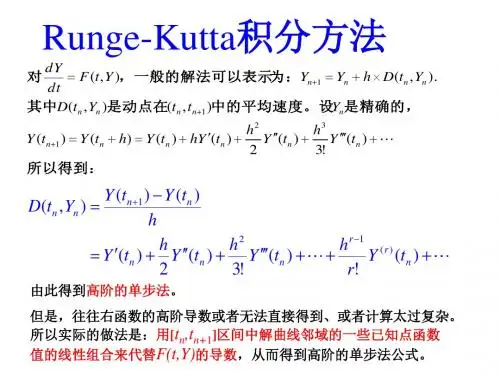
龙格库塔法推导
- 格式:pdf
- 大小:391.42 KB
- 文档页数:31


数值分析中,龙格-库塔法(Runge-Kutta)是用于模拟常微分方程的解的重要的一类隐式或显式迭代法。
这些技术由数学家卡尔·龙格和马丁·威尔海姆·库塔于1900年左右发明。
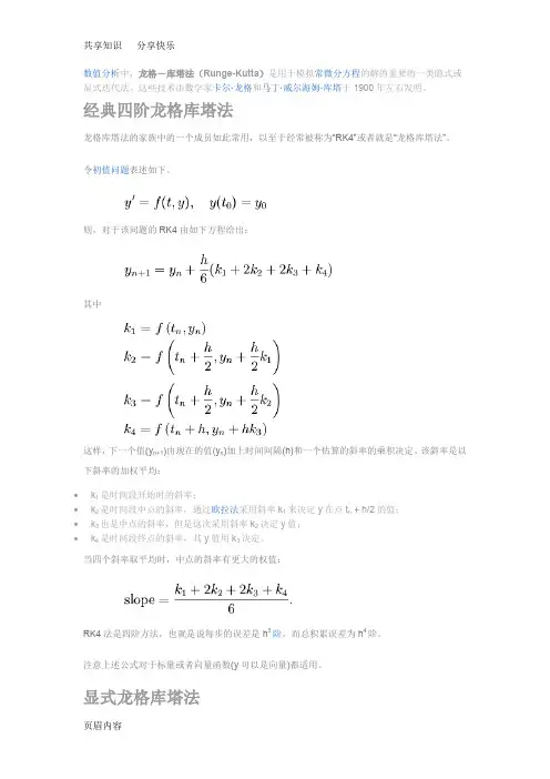
经典四阶龙格库塔法龙格库塔法的家族中的一个成员如此常用,以至于经常被称为“RK4”或者就是“龙格库塔法”。
令初值问题表述如下。
则,对于该问题的RK4由如下方程给出:其中这样,下一个值(y n+1)由现在的值(y n)加上时间间隔(h)和一个估算的斜率的乘积决定。
该斜率是以下斜率的加权平均:∙k1是时间段开始时的斜率;∙k2是时间段中点的斜率,通过欧拉法采用斜率k1来决定y在点t n + h/2的值;∙k3也是中点的斜率,但是这次采用斜率k2决定y值;∙k4是时间段终点的斜率,其y值用k3决定。
当四个斜率取平均时,中点的斜率有更大的权值:RK4法是四阶方法,也就是说每步的误差是h5阶,而总积累误差为h4阶。
注意上述公式对于标量或者向量函数(y可以是向量)都适用。
显式龙格库塔法显示龙格-库塔法是上述RK4法的一个推广。
它由下式给出其中如果要求方法有精度p则还有相应的条件,也就是要求舍入误差为O(h p+1)时的条件。
这些可以从舍入误差本身的定义中导出。
例如,一个2阶精度的2段方法要求b1 + b2 = 1, b2c2 = 1/2, 以及b2a21 = 1/2。
在Matlab下输入:edit,然后将下面两行百分号之间的内容,复制进去,保存%%%%%%%%%%%%%%%%%%%%%%%%%%%%%%%%%%%%%% %%%%%%%%%%%%%%%%%%%%%%%%%%%%%function dxdt=ode_Miss_ghost(t,x)%分别用x(1),x(2),x(3),x(4)代替N1,P1,N2,P2N1=x(1);P1=x(2);N2=x(3);P2=x(4);K=2;tau_c=3e-9;tan_p=6e-12;beta =5e-5;delta=0.692;eta =0.0001;fm =8e6;Ith =26e-3;Ib =1.5*Ith;Im =0.3*Ith;I1=Ib+Im*sin(2*pi*fm*t)+K*P2;I2=Ib+Im*sin(2*pi*fm*t)+K*P1;dxdt=[(I1/Ith-N1-(N1-delta)/(1-delta)*P1)/tau_e;((N1-delta)/(1-delta)*(1-eta*P1)*P1-P1+beta*N1)/tau_p;(I2/Ith-N2-(N2-delta)/(1-delta)*P2)/tau_e;((N2-delta)/(1-delta)*(1-eta*P2)*P2-P2+beta*N2)/tau_p;]; %%%%%%%%%%%%%%%%%%%%%%%%%%%%%%%%%%%%%% %%%%%%%%%%%%%%%%%%%%%%%%%%%%%%在Matlab下面输入:t_start=0;t_end=2e-9;y0=[1e-3;1e-4;0;0]; %初值[x,y]=ode15s('ode_Miss_ghost',[0,t_end],y0);plot(x,y);legend('N1','P1','N2','P2');xlabel('x');Mathlab定步长龙格-库塔法[345阶]、自适应步长rkf45经常看到很多朋友问定步长的龙格库塔法设置问题,下面吧定步长三阶、四阶、五阶龙格库塔程序贴出来,有需要的可以看看ODE3 三阶龙格-库塔法CODE:function Y = ode3(odefun,tspan,y0,varargin)%ODE3 Solve differential equations with a non-adaptive method of order 3.% Y = ODE3(ODEFUN,TSPAN,Y0) with TSPAN = [T1, T2, T3, ... TN] integrates% the system of differential equations y' = f(t,y) by stepping from T0 to% T1 to TN. Function ODEFUN(T,Y) must return f(t,y) in a column vector.% The vector Y0 is the initial conditions at T0. Each row in the solution% array Y corresponds to a time specified in TSPAN.%% Y = ODE3(ODEFUN,TSPAN,Y0,P1,P2...) passes the additional parameters% P1,P2... to the derivative function as ODEFUN(T,Y,P1,P2...).%% This is a non-adaptive solver. The step sequence is determined by TSPAN% but the derivative function ODEFUN is evaluated multiple times per step.% The solver implements the Bogacki-Shampine Runge-Kutta method of order 3.%% Example% tspan = 0:0.1:20;% y = ode3(@vdp1,tspan,[2 0]);% plot(tspan,y(:,1));% solves the system y' = vdp1(t,y) with a constant step size of 0.1, % and plots the first component of the solution.%if ~isnumeric(tspan)error('TSPAN should be a vector of integration steps.');endif ~isnumeric(y0)error('Y0 should be a vector of initial conditions.');endh = diff(tspan);if any(sign(h(1))*h <= 0)error('Entries of TSPAN are not in order.')endtryf0 = feval(odefun,tspan(1),y0,varargin{:});catchmsg = ['Unable to evaluate the ODEFUN at t0,y0. ',lasterr];error(msg);endy0 = y0(:); % Make a column vector.if ~isequal(size(y0),size(f0))error('Inconsistent sizes of Y0 and f(t0,y0).');endneq = length(y0);N = length(tspan);Y = zeros(neq,N);F = zeros(neq,3);Y(:,1) = y0;for i = 2:Nti = tspan(i-1);hi = h(i-1);yi = Y(:,i-1);F(:,1) = feval(odefun,ti,yi,varargin{:});F(:,2) = feval(odefun,ti+0.5*hi,yi+0.5*hi*F(:,1),varargin{:});F(:,3) = feval(odefun,ti+0.75*hi,yi+0.75*hi*F(:,2),varargin{:});Y(:,i) = yi + (hi/9)*(2*F(:,1) + 3*F(:,2) + 4*F(:,3));endY = Y.';ODE4 四阶龙格-库塔法CODE:function Y = ode4(odefun,tspan,y0,varargin)%ODE4 Solve differential equations with a non-adaptive method of order 4.% Y = ODE4(ODEFUN,TSPAN,Y0) with TSPAN = [T1, T2, T3, ... TN] integrates % the system of differential equations y' = f(t,y) by stepping from T0 to% T1 to TN. Function ODEFUN(T,Y) must return f(t,y) in a column vector.% The vector Y0 is the initial conditions at T0. Each row in the solution% array Y corresponds to a time specified in TSPAN.%% Y = ODE4(ODEFUN,TSPAN,Y0,P1,P2...) passes the additional parameters % P1,P2... to the derivative function as ODEFUN(T,Y,P1,P2...).%% This is a non-adaptive solver. The step sequence is determined by TSPAN % but the derivative function ODEFUN is evaluated multiple times per step.% The solver implements the classical Runge-Kutta method of order 4.%% Example% tspan = 0:0.1:20;% y = ode4(@vdp1,tspan,[2 0]);% plot(tspan,y(:,1));% solves the system y' = vdp1(t,y) with a constant step size of 0.1,% and plots the first component of the solution.%if ~isnumeric(tspan)error('TSPAN should be a vector of integration steps.');endif ~isnumeric(y0)error('Y0 should be a vector of initial conditions.');endh = diff(tspan);if any(sign(h(1))*h <= 0)error('Entries of TSPAN are not in order.')endtryf0 = feval(odefun,tspan(1),y0,varargin{:});catchmsg = ['Unable to evaluate the ODEFUN at t0,y0. ',lasterr]; error(msg);endy0 = y0(:); % Make a column vector.if ~isequal(size(y0),size(f0))error('Inconsistent sizes of Y0 and f(t0,y0).');endneq = length(y0);N = length(tspan);Y = zeros(neq,N);F = zeros(neq,4);Y(:,1) = y0;for i = 2:Nti = tspan(i-1);hi = h(i-1);yi = Y(:,i-1);F(:,1) = feval(odefun,ti,yi,varargin{:});F(:,2) = feval(odefun,ti+0.5*hi,yi+0.5*hi*F(:,1),varargin{:}); F(:,3) = feval(odefun,ti+0.5*hi,yi+0.5*hi*F(:,2),varargin{:}); F(:,4) = feval(odefun,tspan(i),yi+hi*F(:,3),varargin{:});Y(:,i) = yi + (hi/6)*(F(:,1) + 2*F(:,2) + 2*F(:,3) + F(:,4));endY = Y.';定步长RK4(自编):CODE:function Y=RungeKutta4(f,xn,y0)% xn=0:.1:1;% y0=1;% y_n=[];% f=@(X1,Y1) Y1-2*X1/Y1;y_n=[];h=diff(xn(1:2));for i=1:length(xn)-1K1=f(xn(i),y0);K2=f(xn(i)+h/2,y0+h*K1/2);K3=f(xn(i)+h/2,y0+h*K2/2);K4=f(xn(i)+h,y0+h*K3);y_n=[y_n;y0+h/6*(K1+2*K2+2*K3+K4)];y0=y_n(end);endY=y_n;ODE5 五阶龙格-库塔法CODE:function Y = ode5(odefun,tspan,y0,varargin)%ODE5 Solve differential equations with a non-adaptive method of order 5.% Y = ODE5(ODEFUN,TSPAN,Y0) with TSPAN = [T1, T2, T3, ... TN] integrates % the system of differential equations y' = f(t,y) by stepping from T0 to% T1 to TN. Function ODEFUN(T,Y) must return f(t,y) in a column vector.% The vector Y0 is the initial conditions at T0. Each row in the solution% array Y corresponds to a time specified in TSPAN.%% Y = ODE5(ODEFUN,TSPAN,Y0,P1,P2...) passes the additional parameters % P1,P2... to the derivative function as ODEFUN(T,Y,P1,P2...).%% This is a non-adaptive solver. The step sequence is determined by TSPAN % but the derivative function ODEFUN is evaluated multiple times per step.% The solver implements the Dormand-Prince method of order 5 in a general % framework of explicit Runge-Kutta methods.%% Example% tspan = 0:0.1:20;% y = ode5(@vdp1,tspan,[2 0]);% plot(tspan,y(:,1));% solves the system y' = vdp1(t,y) with a constant step size of 0.1,% and plots the first component of the solution.if ~isnumeric(tspan)error('TSPAN should be a vector of integration steps.');endif ~isnumeric(y0)error('Y0 should be a vector of initial conditions.');endh = diff(tspan);if any(sign(h(1))*h <= 0)error('Entries of TSPAN are not in order.')endtryf0 = feval(odefun,tspan(1),y0,varargin{:});catchmsg = ['Unable to evaluate the ODEFUN at t0,y0. ',lasterr];error(msg);endy0 = y0(:); % Make a column vector.if ~isequal(size(y0),size(f0))error('Inconsistent sizes of Y0 and f(t0,y0).');endneq = length(y0);N = length(tspan);Y = zeros(neq,N);% Method coefficients -- Butcher's tableau%% C | A% --+---% | BC = [1/5; 3/10; 4/5; 8/9; 1];A = [ 1/5, 0, 0, 0, 03/40, 9/40, 0, 0, 044/45 -56/15, 32/9, 0, 019372/6561, -25360/2187, 64448/6561, -212/729, 0 9017/3168, -355/33, 46732/5247, 49/176, -5103/18656];B = [35/384, 0, 500/1113, 125/192, -2187/6784, 11/84]; % More convenient storageA = A.';B = B(:);nstages = length(B);F = zeros(neq,nstages);Y(:,1) = y0;for i = 2:Nti = tspan(i-1);hi = h(i-1);yi = Y(:,i-1);% General explicit Runge-Kutta frameworkF(:,1) = feval(odefun,ti,yi,varargin{:});for stage = 2:nstageststage = ti + C(stage-1)*hi;ystage = yi + F(:,1:stage-1)*(hi*A(1:stage-1,stage-1));F(:,stage) = feval(odefun,tstage,ystage,varargin{:});endY(:,i) = yi + F*(hi*B);endY = Y.';-------------------------------------------------------------------------------------------------------------------自适应步长RKF45(相当于ode45)ODE45 是4阶方法提供候选解,5阶方法控制误差。
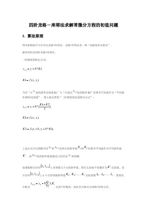
四阶龙格-库塔法求解常微分方程的初值问题1.算法原理对于一阶常微分方程组的初值问题⎪⎪⎪⎩⎪⎪⎪⎨⎧=⋯⋯==⋯⋯=⋯⋯⋯⋯=⋯⋯=0020********'212'2211'1)(,,)(,)())(,),(),(,()())(,),(),(,()())(,),(),(,()(n n n n n n n y x y y x y y x y x y x y x y x f x y x y x y x y x f x y x y x y x y x f x y , 其中b x a ≤≤。
若记Tn Tn Tn y x f y x f y x f y x f y y y y x y x y x y y x y )),(,),,(),,((),(),,,())(),(),(()(2102010021⋯⋯=⋯⋯=⋯⋯=,,则可将微分方程组写成向量形式⎩⎨⎧=≤≤=0')()),(,()(y a y b x a x y x f x y微分方程组初值问题在形式上和单个微分方程处置问题完全相同,只是数量函数在此变成了向量函数。
因此建立的单个一阶微分方程初值问题的数值解法,可以完全平移到求解一阶微分方程组的初值问题中,只不过是将单个方程中的函数转向向量函数即可。
标准4阶R-K 法的向量形式如下:⎪⎪⎪⎪⎩⎪⎪⎪⎪⎨⎧++=++=++==++++=+),()21,2()21,2(),()22(61342312143211K y h x hf K K y h x hf K K y h x hf K y x hf K K K K K y y n n n n n n n n n n 其分量形式为n j K y K y K y h x hf K K y K y K y h x hf K K y K y K y h x hf K y y y x hf K K K K K y y n ni i i i j j n nii i i j j n nii i i j j ni i i i j j j j j j i j i j ,,2,1).,,,;(),2,2,2;2(),2,2,2;2(),,,,;(),22(6132321314222212131212111221143211,1,⋯⋯=⎪⎪⎪⎪⎩⎪⎪⎪⎪⎨⎧+⋯⋯+++=+⋯⋯+++=+⋯⋯+++=⋯⋯=++++=++,,2.程序框图3.源代码%该函数为四阶龙格-库塔法function [x,y]=method(df,xspan,y0,h)%df为常微分方程,xspan为取值区间,y0为初值向量,h为步长x=xspan(1):h:xspan(2);m=length(y0);n=length(x);y=zeros(m,n);y(:,1)=y0(:);for i=1:n-1k1=feval(df,x(i),y(:,i));k2=feval(df,x(i)+h/2,y(:,i)+h*k1/2);k3=feval(df,x(i)+h/2,y(:,i)+h*k2/2);k4=feval(df,x(i)+h,y(:,i)+h*k3);y(:,i+1)=y(:,i)+h*(k1+2*k2+2*k3+k4)/6;end%习题9.2clear;xspan=[0,1];%取值区间h=0.05;%步长y0=[-1,3,2];%初值df=@(x,y)[y(2);y(3);y(3)+y(2)-y(1)+2*x-3];[xt,y]=method(df,xspan,y0,h)syms t;yp=t*exp(t)+2*t-1;%微分方程的解析解yp1=xt.*exp(xt)+2*xt-1%计算区间内取值点上的精确解[xt',y(1,:)',yp1']%y(1,:)为数值解,yp1为精确解ezplot(yp,[0,1]);%画出解析解的图像hold on;plot(xt,y(1,:),'r');%画出数值解的图像4.计算结果。
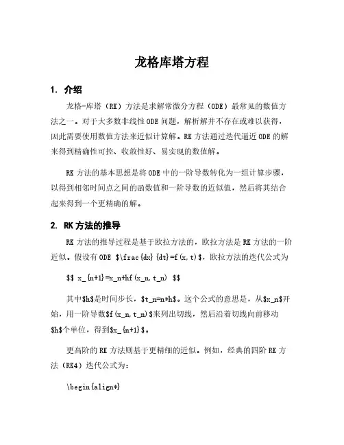
龙格库塔方程1.介绍龙格-库塔(RK)方法是求解常微分方程(ODE)最常见的数值方法之一。
对于大多数非线性ODE问题,解析解并不存在或难以获得,因此需要使用数值方法来近似计算解。
RK方法通过迭代逼近ODE的解来得到精确性可控、收敛性好、易实现的数值解。
RK方法的基本思想是将ODE中的一阶导数转化为一组计算步骤,以得到相邻时间点之间的函数值和一阶导数的近似值,然后将其结合起来得到一个更精确的解。
2.RK方法的推导RK方法的推导过程是基于欧拉方法的,欧拉方法是RK方法的一阶近似。
假设有ODE$\frac{dx}{dt}=f(x,t)$,欧拉方法的迭代公式为$$x_{n+1}=x_n+hf(x_n,t_n)$$其中$h$是时间步长,$t_n=n*h$。
这个公式的意思是,从$x_n$开始,用一阶导数$f(x_n,t_n)$来列出切线,然后沿着切线向前移动$h$个单位,得到$x_{n+1}$。
更高阶的RK方法则基于更精细的近似。
例如,经典的四阶RK方法(RK4)迭代公式为:\begin{align*}k_1&=f(x_n,t_n)\\k_2&=f(x_n+\frac{h}{2}k_1,t_n+\frac{h}{2})\\k_3&=f(x_n+\frac{h}{2}k_2,t_n+\frac{h}{2})\\k_4&=f(x_n+h k_3,t_n+h)\\x_{n+1}&=x_n+\frac{h}{6}(k_1+2k_2+2k_3+k_4)\end{align*}其中,$k_1$是欧拉方法的一阶导数解,依次计算得到更高阶的导数近似值$k_2-k_4$。
3.RK方法的优势RK方法与其他数值方法相比具有众多优点。
首先,RK方法的精度可控。
通过增加迭代次数或者近似阶次,RK 方法可以获得任意高的精度。
这个特性非常适用于涉及长时间尺度和小尺度特征的问题,例如天气预报,需要同时精确地处理地球的自转和大气的扰动。
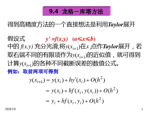
龙格-库塔(Runge-Kutta)公式是一种常用于数值解求微分方程的方法,其中包括了多种不同类型的龙格-库塔公式.
其中最常见的是四阶龙格-库塔公式(Runge-Kutta 4th order method),这种方法通过在当前时刻的函数值和当前时刻的导函数的近似值计算下一时刻的函数值。
它的计算公式如下:
k1 = hf(xn, yn)
k2 = hf(xn + h/2, yn + k1/2)
k3 = hf(xn + h/2, yn + k2/2)
k4 = hf(xn + h, yn + k3)
yn+1 = yn + (k1 + 2k2 + 2k3 + k4)/6
xn+1 = xn + h
其中k1,k2,k3,k4 是近似值,f(x,y)是微分方程,xn, yn 是当前时刻的函数值,xn+1, yn+1 是下一时刻的函数值, h是时间步长.
这种方法具有较高的精度,并且易于实现,但在求解某些类型的方程时,会存在稳定性问题.
除此之外,还有其他类型的龙格-库塔公式,比如二阶、三阶等等,它们也有各自的适用条件.。
⼆阶龙格库塔公式推导_⼆阶龙格库塔公式.ppt⼆阶龙格库塔公式第⼀节 常微分⽅程 第⼆节 欧拉⽅法 第三节 龙格—库塔法 在上⼀节中,我们得到了⼀些求微分⽅程近似解的数值⽅法,这些⽅法的局部截断误差较⼤,精度较低,我们希望得到有更⾼阶精度的⽅法。
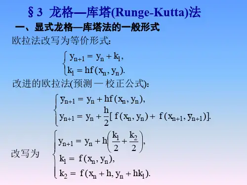
⼀阶龙格—库塔⽅法 如果以y(x)在xi处的斜率作为y(x)在 [xi,xi+1]上的平均斜率k*,即 ⼆阶龙格—库塔⽅法 在[xi,xi+1]上取两点xi,xi+p(0< p≤1)的斜率值k1,k2的线性组合λ1k1+λ2k2作为k*的近似值(λ1、λ2为待定常数),此公式⼀般形式可写成 这就是⼆阶龙格—库塔法公式。
三阶龙格—库塔公式 为了提⾼精度,考虑在[xi,xi+1]上取三点xi,xi+p,xi+q的斜率值分别为k1,k2,k3,将k1,k2,k3的线性组合作为平均斜率k*的近似值,其中 k* 这就是欧拉法. 则得 其中k1 = f (xi,yi),k2为[xi,xi+1]内任意⼀点xi+p = xi+ ph (0< p≤1) 的斜率f (xi+p,y(xi+p))。
由于y (xi+p)并没有给出,所以先应该求y(xi+p),仿照改进欧拉公式的构造思想,得到 (8-7) 这样构造出的公式为 k1 k2 k* 公式中含有三个参数λ1,λ2和p,如果我们适当选取参数的值,可以使公式的局部截断误差为O(h3)。
对k1和k2作泰勒展开 代⼊(8-7)得 (*) ⼜ y (x)在xi处的⼆阶泰勒展开式为 当x = xi+1时, ,有 (**) (**) ⽐较(*)与(**)的系数即可发现, 要使公式(7-7)的局部截断误差满⾜ ,即要求公式具有⼆阶 精度只要下列条件成⽴即可。
(8-8)满⾜条件(8-8)的⼀簇公式统称为 ⼆阶龙格—库塔公式。
特别的,当 塔公式就成为改进欧拉公式。
时,龙格-库 改进欧拉公式就是以y(x)在xi和xi+1 处的斜率k1和k2的算术平均 值作为y(x)在[xi,xi+1]上的 平均斜率k*来进⾏计算的。