第3章 Multisim7高级分析方法

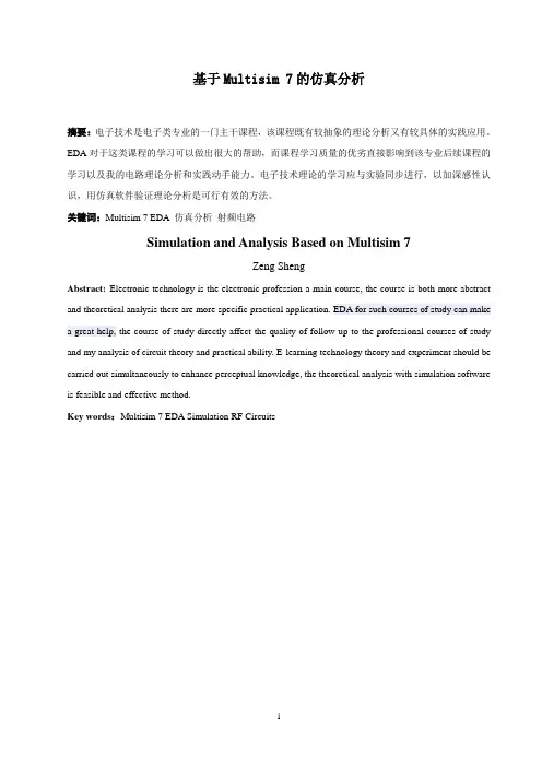
基于Multisim 7的仿真分析摘要：电子技术是电子类专业的一门主干课程，该课程既有较抽象的理论分析又有较具体的实践应用。

EDA对于这类课程的学习可以做出很大的帮助，而课程学习质量的优劣直接影响到该专业后续课程的学习以及我的电路理论分析和实践动手能力。

电子技术理论的学习应与实验同步进行，以加深感性认识，用仿真软件验证理论分析是可行有效的方法。

关键词：Multisim 7 EDA 仿真分析射频电路Simulation and Analysis Based on Multisim 7Zeng ShengAbstract:Electronic technology is the electronic profession a main course, the course is both more abstract and theoretical analysis there are more specific practical application.EDA for such courses of study can make a great help, the course of study directly affect the quality of follow-up to the professional courses of study and my analysis of circuit theory and practical ability.E-learning technology theory and experiment should be carried out simultaneously to enhance perceptual knowledge, the theoretical analysis with simulation software is feasible and effective method.Key words：Multisim 7 EDA Simulation RF Circuits第一章绪论 (3)第二章 Multisim 7常用的虚拟仪器及常用的基本分析方法 (4)第三章仿真电路的处理及基于Multisim 7的VHDL仿真知识 (5)第四章基于Multisim 7的射频电路的仿真分析 (6)4.1 引言 (6)4.2 射频电路的基本知识 (7)4.3 RF特性分析 (8)4.4 匹配网络分析 (14)第五章总结分析 (18)第六章致谢 (19)参考文献： (20)第一章绪论电子技术是电子类专业的一门主干课程，该课程既有较抽象的理论分析又有较具体的实践应用。

Multisim7电路设计及仿真应用本文由文库黄健贡献ppt文档可能在WAP端浏览体验不佳。

建议您优先选择TXT，或下载源文件到本机查看。

Multisim 7电路设计及仿真应用电路设计及仿真应用Multisim 7 概述完整的电路系统设计、仿真工具；设计功能：Schematic & HDL仿真功能：SPICE VHDL/Verilog RF CoCo-simulation虚拟仪表及分析功能以及3 虚拟仪表及分析功能以及3D效果。

Multisim 7 特色所见即所得的设计环境；互动式的仿真界面；动态显示元件（如LED，动态显示元件（如LED，七段显示器等）；具有3 具有3D效果的仿真电路；虚拟仪表(包括Agilent仿真仪表）；虚拟仪表(包括Agilent仿真仪表）；分析功能与图形显示窗口。

操作环境环境参数设定Options/Preferences… ptions/P绘制电路取用元件：从元器件库中取用所需元件；摆放元件：调整元件的位置与方向；线路连接：连接元件的引脚。

元件工具栏电源按钮件按钮元本基二极管按钮钮按管体晶拟元件模元器件按元器件按钮钮元（件按钮COMS 系列）系列）器（字数他其数混合元器件按钮模指示器件按钮杂射项库元元器器件按按钮钮件频电机置元器件按钮钮按件器元设放置总线按钮钮源按资育教网站按钮按钮74取用元件放置元件——电源元件元素Multisim 7的元件均具有下列元素: 7的元件均具有下列元素:Symbol –元件符号（for Schematic）Schematic）Model –元件模型（for Simulation）Simulation）Footprint –元件外型（for Layout）Layout）Electronic Parameter–电子元件参数Parameter–User Defined Info. –使用者自定资讯Pin model—管脚模型model—General—General—元件描述取用元件取用元件-元件属性对话框在元件上双击鼠标左键开启属性对话框Label：Label：修改元件序号、标识；Display：Display：设置元件标识是否显示；Value：Value：设定元件参数值；Fault：Fault：设定元件故障。

第3章Multisim7的元件库在所有电路仿真软件中，都需要一个仿真元件库以存放和管理仿真元件，仿真元件库中元件多少、模型的精确度将对仿真结果有着较大的影响。

本章将主要介绍Multisim7中元件库及元件的使用、元件库管理及如何在Multisim7中创建新元件等内容。

3.1元件库的管理Multisim7的元件存储在三种不同的数据库中，执行“Tools”/“Database Management”命令即可看到数据库管理信息。

主要包括Multisim Master库、Corporate Library库（仅在专业版中存在）、User库，这三种数据库功能分别说明如下：●Multisim Master库：存放Multisim7提供的所有元件，不能被修改和编辑。

●Corporate Library库：存放被企业或个人修改、创建和选择的元件，能对选择了该库的企业或个人使用和编辑。

主要是方便企业的设计团队共享经常使用的一些特定的元件。

●User库：存放被个人修改、创建和导入的元件，仅能由使用者个人使用和编辑。

该库在刚使用Multisim7时是空的，可以通过导入或由用户自己编辑和创建（详见3.3节）。

如图3-1所示的Multisim Master库和User库中都包含如下13个元件库分类：信号及电源库（Sources）、基本元件库（Basic）、二极管库（Diodes）、晶体管库（Transistors）、模拟元件库（Analog）、TTL元件库（TTL）、CMOS元件库（CMOS）、其它数字元件库（Misc Digital）、混合元件库（Mixed）、显示元件库（Indicators）、其它元件库（Misc）、射频元件库（RF）、机电类元件库（Electro-mechanical），该分类和元件工具栏中的元件库图标相对应。

在Multisim Master库下面的每个分类元件库中，还包括多个元件箱（又称为Family），各种仿真元件放在这些元件箱中以供调用。

Multisim7分析时序逻辑电路摘要：计算机技术的飞速发展，电路可以通过计算机辅助分析和仿真技术来完成设计。

Multisim7软件就是一个专门用于电子线路仿真与设计的 EDA 工具软件。

它具有很强的逻辑仿真功能，将给定的时序逻辑电路图输入计算机后得到时序图，操作简单快捷。

论文中介绍了Multisim7软件以及时序逻辑电路的特点和分析过程，并用例题加以说明。

关键词：Multisim7，时序逻辑电路，逻辑分析仪，信号发生器随着计算机科学与技术突飞猛进的发展，用数字电路进行信号处理的优势也更加突出。

为了充分发挥和利用数字电路在处理上的强大功能，我们可以先将模拟信号按比例转化成数字信号，然后送到数字电路（可以是专用的数字信号处理电路，也可以是通用的计算机）进行处理，最后处理结果根据需要转化为相应的模拟信号输出。

自20世纪70年代开始，这种用数字模拟信号的所谓“数字化”浪潮已经席卷了电子技术几乎所有，所有的应用领域。

Multisim7把整个学习和实验过程都搬到了虚拟实验室中进行，能够使实验电路，仪器以及实验结果等一起直观地展现在学生面前，另外对电路参数调整也极其方便。

本文就采用Multisim7对时序逻辑电路进行分析。

一、Multisim7软件的介绍Multisim7是由加拿大IIT(Interaction Image Technologies)公司推出的大型设计工具软件。

Multisim7 仿真软件的前身是EWB, 又称电子工作台（Electronics Work bench），它是由加拿大IIT 公司20 世纪80 年代推出的电子电路设计和仿真软件，一经推出就受到好评，尤其在教育领域取得了巨大的成功。

EWB 软件具有界面直观，操作方便等优点，创建电路、选用元件和测试仪器均可以直接通过元件库和仪器库选取。

EWB系列软件经过了多个版本的演变，在2003年IIT 公司推出了Multisim7版本，较之以前的版本功能更加齐全，应用也更加广泛。

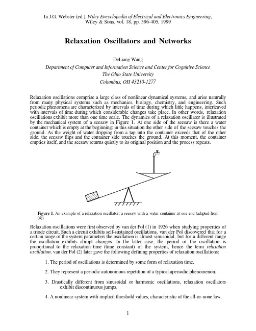
In J.G. Webster (ed.), Wiley Encyclopedia of Electrical and Electronics Engineering,Wiley & Sons, vol. 18, pp. 396-405, 1999Relaxation Oscillators and NetworksDeLiang WangDepartment of Computer and Information Science and Center for Cognitive ScienceThe Ohio State UniversityColumbus, OH 43210-1277Relaxation oscillations comprise a large class of nonlinear dynamical systems, and arise naturally from many physical systems such as mechanics, biology, chemistry, and engineering. Such periodic phenomena are characterized by intervals of time during which little happens, interleaved with intervals of time during which considerable changes take place. In other words, relaxation oscillations exhibit more than one time scale. The dynamics of a relaxation oscillator is illustrated by the mechanical system of a seesaw in Figure 1. At one side of the seesaw is there a water container which is empty at the beginning; in this situation the other side of the seesaw touches the ground. As the weight of water dripping from a tap into the container exceeds that of the other side, the seesaw flips and the container side touches the ground. At this moment, the container empties itself, and the seesaw returns quictly to its original position and the process repeats.Figure 1. An example of a relaxation oscillator: a seesaw with a water container at one end (adapted from(4)).Relaxation oscillations were first observed by van der Pol (1) in 1926 when studying properties of a triode circuit. Such a circuit exhibits self-sustained oscillations. van der Pol discovered that for a certain range of the system parameters the oscillation is almost sinusoidal, but for a different range the oscillation exhibits abrupt changes. In the latter case, the period of the oscillation is proportional to the relaxation time (time constant) of the system, hence the term relaxation oscillation. van der Pol (2) later gave the following defining properties of relaxation oscillations:1. The period of oscillations is determined by some form of relaxation time.2. They represent a periodic autonomous repetition of a typical aperiodic phenomenon.3. Drastically different from sinusoidal or harmonic oscillations, relaxation oscillatorsexhibit discontinuous jumps.4. A nonlinear system with implicit threshold values, characteristic of the all-or-none law.A variety of biological phenomena can be characterized as relaxation oscillations, ranging from heartbeat, neuronal activity, to population cycles; the English physiologist A.V. Hill (3) even stated that relaxation oscillations are the type of oscillations that governs all periodic phenomena in physiology.Givenrelaxation oscillations. TheimportantRELAXATION OSCILLATORSoscillators.arewith electrical circuits.van der Pol oscillator˙˙x+x=c(1−x2)˙x Figure 2. Phase portrait and trajectory of a van der Pol oscillator. A Phase portrait. The x nullcline is the cubic curve, and the y nullcline is the y axis. Arrows indicate phase flows. B limit cycle orbit. The limit cycle is labeled as pqrs, and the arrowheadswhere c > 0 is a parameter. This second-order differential equation can be transformed to a two variable first-order differential equation,˙x=c(y−f(x))(2a)˙y=−x/c(2b)Here f(x) = -x + x3/3. The x nullcline, ˙x = 0, is a cubic curve, while the y nullcline, ˙y = 0, is the y axis. As shown in Fig. 2A, the two nullclines intersect along the middle branch of the cubic, and the resulting fixed point is unstable as indicated by the flow field in the phase plane of Fig. 2A. This equation yields a periodic solution.As c » 1, Eq. (2) yields two time scales: a slow time scale for the y variable and a fast time scale for the x variable. As a result, Eq. (2) becomes the van der Pol oscillator that produces a relaxation oscillation. The limit cycle for the van der Pol oscillator is given in Fig. 2B, and it is composed of four pieces, two slow ones indicated by pq and rs, and two fast ones indicated by qr and sp. In other words, motion along the two branches of the cubic is slow compared to fast alternations, or jumps, between the two branches. Fig. 2C shows x activity of the oscillator with respect to time, where two time scales are clearly indicated by relatively slow changes in x activity interleaving with fast changes.FitzHugh-Nagumo oscillatorBy simplifying the classical Hodgkin-Huxley equations (7) for modeling nerve membranes and action potential generation, FitzHugh (8) and Nagumo et al. (5) gave the following two-variable equation, widely known as the FitzHugh-Nagumo model,˙x=c(y−f(x)+I)(3a)˙y=−(x+by−a)/c(3b) where f(x) is as defined in Eq. (2), I is the injected current, and a, b, and c are system parameters satisfying the conditions: 1 > b > 0, c2 > b, and 1 > a > 1 – 2b/3. In neurophysiological terms, x corresponds to the neuronal membrane potential, and y plays the aggregate role of three variables in the Hodgkin-Huxley equations. Given that the x nullcline is a cubic and the y nullcline is linear, the FitzHugh-Nagumo equation is mathematically similar to the van der Pol equation. Typical relaxation oscillation with two time scales occurs when c » 1. Because of the three parameters and the external input I, the FitzHugh-Nagumo oscillator has additional flexibility. Depending on parameter values, the oscillator can exhibit a stable steady state or a stable periodic orbit. With a perturbation by external stimulation, the steady state can become unstable and be replaced by an oscillation; the steady state is thus referred to as the excitable state.Morris-Lecar oscillatorIn modeling voltage oscillations in barnacle muscle fibers, Morris and Lecar (9) proposed the following equation,˙x=−g Ca m∞(x)(x−1)−g K y(x−x K)−g L(x−x L)+I(4a)˙y=−ε(y∞(x)−y)/τy(x)(4b) wherem ∞(x )=[1+tanh((x −x 1)/x 2)]/2y ∞(x )=[1+tanh((x −x 3)/x 4)]/2τy (x )=1/cosh[(x −x 3)/(2x 4)]and x 1, x 2, x 3, x 4, g Ca , g K , g L , x K , and x L are parameters. Ca stands for calcium, K for potassium, L for leak, and I is the injected current. The parameter ε controls relative time scales of x and y . Like Eq. (4), the Morris-Lecar oscillator is closely related to the Hodgkin-Huxley equations, and it is used as a two-variable description of neuronal membrane properties or the envelope of an oscillating burst (10). The x variable corresponds to the membrane potential, and y corresponds to the state of activation of ionic channels.The x nullcline of Eq. (4) resembles a cubic and the y nullcline is a sigmoid curve. When ε isTerman-Wang oscillatorconsiderations, the following equation,˙x=f (x )−y +I ˙y=ε(g (x )−y )where f(x) = 3x – x 3 + 2, g(x) = α/β)), and I represents oscillator. Thus x nullcline is a sigmoid, where αparameters. When εrelaxation oscillator. When I βperiodic solution alternates between and active (high x behavior. As shown in Fig. respectively. If I spends in these two phases. A largervan der Pol and FitzHugh-Nagumo equations. In neuronal terms, the x variable in Eq. (5) corresponds to the membrane potential, and y the state for channel activation or inactivation.NETWORKS OF RELAXATION OSCILLATORSIn late eighties, neural oscillations about 40 Hz were discovered to in the visual cortex (12-13). The experimental findings can be summarized as the following: (1) neural oscillations are triggered by appropriate sensory stimulation, and thus the oscillations are stimulus-dependent; (2) long-range synchrony with zero phase-lag occurs if the stimuli appear to form a coherent object; (3) no synchronization occurs if the stimuli appear to be unrelated. These intriguing observations are consistent with the temporal correlation theory (14), which states that in perceiving a coherent object the brain links various feature detecting neurons via temporal correlation among the firing activities of these neurons.Since the discovery of coherent oscillations in the visual cortex and other brain areas, neural oscillations and synchronization of oscillator networks have been extensively studied. Most of these models are based on sinusoidal or harmonic oscillators and rely on all-to-all connectivity to reach synchronization across the network. In fact, according to the Mermin and Wagner theorem (15) in statistical physics, no synchrony exists in one- or two-dimensional locally coupled isotropic Heisenberg oscillators, which are similar to harmonic oscillators. However, all-to-all connectivity(16)modulationrelaxationand in this case the effect of the excitatory coupling is to raise the cubic of the other oscillator by a fixed amount.Let us explain the mechanism of fast threshold modulation using the Terman-Wang oscillator as an example. The two oscillators are denoted by o1 = (x1, y1) and o2 = (x2, y2), which are initially in the silent phase and close to each other with o1 leading the way as illustrated in Fig. 4. Figure 4 shows the solution of the oscillator system in the singular limit ε→ 0. The singular solution consists of several pieces. The first piece is when both oscillators move along LB of the uncoupled cubic, denoted as C. This piece lasts until o1 reaches the left knee of C, LK, at t = t1. The second piece begins when o1 jumps up to RB, and the excitatory coupling from o1 to o2 raises the cubic for o2 from C to C E as shown in the figure. Let LK E and RK E denote the left and right knees of C E. If |y1 - y2| is relatively small, then o2 lies below LK E and jumps up. Since these interactions take place in fast time, the oscillators are effectively synchronized in jumping up. As a result the cubic for o1 is raised to C E as well. The third piece is when both oscillators lie on RB and evolve in slow time. Note that the ordering in which the two oscillators track along RB is reversed and now o2 leads the way. The third piece lasts until o2 reaches RK E at t = t2. The fourth piece starts when o2 jumps down to LB. With o2 jumping down, the cubic for o1 is lowered to C. At this time, if o1 lies above RK, as shown in Fig. 4, o1 jumps down as well and both oscillators are now in the silent phase. Once both oscillators are on LB, the above analysis repeats.Based on the fast threshold modulation mechanism, Somers and Kopell further proved a theorem that the synchronous solution in the oscillator pair has a domain of attraction in which the approach to synchrony has a geometric (or exponential) rate (16). The Somers-Kopell theorem is based on comparing the evolution rates of the slow variable right before and after a jump, which are determined by the vertical distances of an oscillator to the y nullcline (see Fig. 4).A network of locally coupled oscillatorsIn the same paper Somers and Kopell suspected that their analysis extends to a network of relaxation oscillators, and performed numerical simulations with one-dimensional rings to support their suggestion. In a subsequent study, by extending Somers and Kopell analysis, Terman and Wang proved a theorem that for an arbitrary network of locally coupled relaxation oscillators there is a domain of attraction in which the entire network synchronizes at an exponential rate (11).In their analysis, Terman and Wang employed the time metric to describe the distance between oscillators. When oscillators evolve either in the silent phase or the active phase, their distances in y in the Euclidean metric change; however, their distances in the time metric remain constant. On the other hand, when oscillators jump at the same time (in slow time), their y distances remain unchanged while their time distances change. Terman and Wang also introduced the condition that the sigmoid for the y nullcline (again consider the Terman-Wang oscillator) is very close to a step function (11), which is the case when β in Eq. (5) is chosen to be very small. This condition implies that in the situation with multiple cubics the rate of evolution of a slow variable does not depend on which cubic it tracks along.LEGION networks: Selective gatingA natural and special form of the temporal correlation theory is oscillatory correlation (19), whereby each object is represented by synchronization of the oscillator group corresponding to the object and different objects in a scene are represented by different oscillator groups which are desynchronized from each other. There are two fundamental aspects in the oscillatory correlationtheory: synchronization and desynchronization. Extending their results on synchronizing locally coupled relaxation oscillators, Terman and Wang used a global inhibitory mechanism to achieve desynchronization (11). The resulting network is called LEGION, to stand for Locally Excitatory Globally Inhibitory Oscillator Networks (19).The original description of LEGION is based on Terman-Wang oscillators, and basic mechanisms extend to other relaxation oscillator models. Each oscillator i is defined as˙xi = f (x i )−y i +I i +S i +ρ(6a)˙yi =ε(g (x i )−y i )(6b)Here f(x) and g(x) are as given in Eq. (5). The parameter ρ denotes the amplitude of Gaussiannoise; to reduce the chance of self-generating oscillations the mean of noise is set to -ρ. In addition to test robustness, noise plays the role of assisting desynchronization. The term S i denotes the overall input from other oscillators in the network:S i = ∑k ∈N (i )W ik H (x k – θx ) – W z H (z – θz )(7)where W ik is the dynamic connection weight from k to i , and N(i) is the set of the adjacent oscillators that connect to i . In a two-dimensional (2-D) LEGION network, N(i) in the simplest case contains four immediate neighbors except on boundaries where no wrap-around is used,thus forming a 2-D grid. This architecture is shown in Fig. 5. H stands for the Heaviside function, defined as H (v ) = 1 if v ≥ 0 and H (v ) = 0 if v < 0. θx is a threshold above which an oscillator can affect its neighbors. W z is the weight of inhibition from the global inhibitor z , whose activity is defined as˙z= φ (σ∞ – z ) (8)where φ is a parameter. The quantity σ∞ = 1 if x i ≥ θz for at least one oscillator i , and σ∞ = 0otherwise. Hence θz (see also Eq. (7))represents a threshold.The dynamic weights W ik 's are formed on the basis of permanent weights T ik 's according to the mechanism of dynamic normalization (20-21), which ensures that each oscillator has equal overall weights of dynamic connections, W T , from its neighborhood. According to reference (11), weight normalization is not a necessary condition for LEGION to work, but it improves the quality of synchronization. Moreover, based on external input W ik can be determined at the start of simulation.To illustrate how desynchronization between blocks of oscillators is achieved in a LEGION network, let us consider an example with two oscillators that are coupled only through the global< y2thefirst one lasts until o1both oscillators are on LB, zpiece starts when o1crosses θz, σ∞on the fast time scale. When zcubic corresponding to both o1from C to C Zis when o1P Zthat o2→P Z, and o2o1 is on RB, which lasts until o1knee of C Z at t = t2o1 jumps down to LB. When o10 in fast time. When zcorresponding to both o1 and oimmediately. Otherwise both o1terminates when o21 and o2 are never in the active phase simultaneously. In general, LEGION exhibits a mechanism of selective gating, whereby an oscillator, say o i, jumping to its active phase quickly activates the global inhibitor, which selectively prevents the oscillators representing different blocks from jumping up, without affecting o i's ability in recruiting the oscillators of the same block because of local excitation. With the selective gating mechanism, Terman and Wang proved the following theorem. For a LEGION network there is a domain of parameters and initial conditions in which the network achieves both synchronization within blocks of oscillators and desynchronization between different blocks in no greater than N cycles of oscillations, where N is the number of patterns in an input scene. In other words, both synchronization and desynchronization are achieved rapidly.The following simulation illustrates the process of synchronization and desynchronization in LEGION (19). Four patterns - two O's, one H, and one I, forming the word OHIO - are simultaneously presented to a 20x20 LEGION network as shown in Figure 7A. Each pattern is a connected region, but no two patterns are connected to each other. The oscillators under stimulation become oscillatory, while those without stimulation remain excitable. The parameter ρis set to represent 10% noise compared to the external input. The phases of all the oscillators on the grid are randomly initialized. Fig. 7B-7F shows the instantaneous activity (snapshot) of the network at various stages of dynamic evolution. Fig. 7B shows a snapshot of the network at thebeginning of the simulation, displaying the random initial conditions. Fig. 7C shows a snapshotshortly afterwards. One can clearly see the effect of synchronization and desynchronization: all the oscillators corresponding to the left O are entrained and have large activity; at the same time, the oscillators stimulated by the other three patterns have very small activity. Thus the left O is segmented from the rest of the input. Figure 7D-F shows subsequent snapshots of the network, where different patterns reach the active phase and segment from the rest. This successive "popout" of the objects continues in an approximately periodic fashion as long as the input stays on. To provide a complete picture of dynamic evolution, Fig. 7G shows the temporal evolution of every oscillator. Synchronization within each object and desynchronization between them are clearly shown in just three oscillation periods, which is consistent with the theorem proven in (11).GLeft OPattern HPattern IRight OInhibitorTimeFigure 7.A A scene composed of four patterns which were presented (mapped) to a 20x20 LEGION network. B A snapshot of the activities of the oscillator grid at the beginning of dynamic evolution. The diameter of each black circle represents the x activity of the corresponding oscillator. C A snapshot taken shortly after the beginning. D Another snapshot taken shortly after C. E Another snapshot taken shortly after D. F Another snapshot taken shortly after E. G The upper four traces show the combined temporal activities of the oscillator blocks representing the four patterns, respectively, and the bottom trace shows the temporal activity of the global inhibitor. The ordinate indicates the normalized x activity of an oscillator. Since the oscillators receiving no external input are excitable during the entire simulation process, they are excluded from the display. The activity of the oscillators stimulated by each object is combined into a single trace in the figure. The differential equations were solved using a fourth-order Runge-Kutta method. (from (19))Time delay networksTime delays in signal transmission are inevitable in both the brain and physical systems. In local cortical circuits, for instance, the speed of nerve conduction is less than 1mm/ms such that connected neurons 1 mm apart have a time delay of more than 4% of the period of oscillation assuming 40 Hz oscillations. Since small delays may completely alter the dynamics of differential equations, it is an important to understand how time delays change the behavior, particularly synchronization, of relaxation oscillator networks.Recently, Campbell and Wang (22) studied locally coupled relaxation oscillators with time delays. They revealed the phenomenon of loose synchrony in such networks. Loose synchrony indemonstrates loosely synchronous behavior in a chain of 50 oscillators with a time delay that is 3%of the oscillation period between adjacent oscillators. The phase relations between the oscillators in the chain become stabilized by the third cycle.Two other results regarding relaxation oscillator networks with time delays are worth mentioning.First, Campbell and Wang (22) identified a range of initial conditions in which the maximum time delays between any two oscillators in a locally coupled network can be contained. Second, they found that in LEGION networks with time delay coupling between oscillators, desynchronous solutions for different oscillator blocks are maintained. Thus, the introduction of time delays does not appear to impact the behavior of LEGION in terms of synchrony and desynchrony.APPLICATIONS TO SCENE ANALYSISA natural scene generally contains multiple objects, each of which can be viewed as a group of similar sensory features. A major motivation behind studies on oscillatory correlation is scene analysis, or the segmentation of a scene into a set of coherent objects. Scene segmentation, or perceptual organization, plays a critical role in the understanding of natural scenes. Although humans perform it with apparent ease, the general problem of scene segmentation remains unsolved in sensory and perceptual information processing.Oscillatory correlation provides an elegant and unique way to represent results of segmentation. As illustrated in Fig. 7, segmentation is performed in time ; after segmentation, each segment pops out at a distinct time from the network and different segments alternate in time. On the basis of new insights into synchronization and desynchronization properties in relaxation oscillator networks,several recent studies have directly addressed the scene segmentation problem.Image segmentationWang and Terman (21) have studied LEGION for segmenting real images. In order to perform effective segmentation, LEGION needs to be extended to handle images with noisy regions.Without such extension, LEGION would treat each region, no matter how small it is, as a separate segment, and result in many fragments. A large number of fragments degrade segmentation results, and a more serious problem is that it is difficult for LEGION to produce more than severalpatterns (11). This number depends on the ratio of the times that a single oscillator spends in the silent and active phases; see, for example, Figs.3 and 7. This limit is called the segmentation capacity of LEGION (21). Noisy fragments therefore compete with major image regions for becoming segments, and the major segments may not be extracted as athat a major block must contain at least one oscillator, denoted as a leader, which lies in the center area of a large homogeneous image region. Such an oscillator receives large lateral excitation from its neighborhood, and thus its lateral potential is charged high. A noisy fragment does not contain such an oscillator.More specifically, a new variable p i, denoting the lateral potential for each oscillator i is introduced into the definition of the oscillator (cf. (6)). p i→ 1 if i frequently receives a high weighted sum from its neighborhood, signifying that i is a leader, and the value of p i determines whether or not the oscillator i is a leader. After an initial time period, the only oscillators which can jump up without lateral excitation from other oscillators are the leaders. When a leader jumps up, it spreads its activity to other oscillators within its own block, so they can also jump up. Oscillators not in this block are prevented from jumping up because of the global inhibitor. Without a leader, the oscillators corresponding to noisy fragments cannot jump up beyond the initial period. The collection of all noisy regions is called the background, which is generally discontiguous.Wang and Terman have achieved a number of rigorous results concerning the extended version of LEGION (21). The main analytical result states that the oscillators with low lateral potentials will become excitable after a beginning period, and the asymptotic behavior of each oscillator belonging to a major region is precisely the same as the network obtained by simply removing all noisy regions. Given the Terman-Wang theorem on original LEGION, this implies that after a number of cycles a block of oscillators corresponding to a major region synchronizes, while any two blocks corresponding to different major regions desynchronize. Also, the number of periods required for segmentation is no greater than the number of major regions plus one.For gray-level images, each oscillator corresponds to a pixel. In a simple scheme for setting up lateral connections, two neighboring oscillators are connected with a weight proportional to corresponding pixel similarity. To illustrate typical segmentation results, Fig. 9A displays a gray-level aerial image to be segmented. To speed up simulation with large number of oscillators needed for processing real images, Wang and Terman also abstracted an algorithm that follows LEGION dynamics (21). Fig. 9B shows the result of segmentation by the algorithm. The entire image is segmented into 23 regions, each of which corresponds to a different intensity level in the figure, which indicates the phases of oscillators. In the simulation, different segments rapidly popped out from the image, as similarly shown in Fig. 7. As can be seen from Fig. 9B, most of the major regions were segmented, including the central lake, major parkways, and various fields. The black scattered regions in the figure represent the background that remains inactive. Due to the use of lateral potentials, all these tiny regions stay in the background.Auditory segregationA listener in a real auditory environment is generally exposed to acoustic energy from different sources. In order to understand the auditory environment, the listener must first disentangle the acoustic wave reaching the ears. This process is referred to as auditory scene analysis, or auditory segregation. According to Bregman (23), auditory scene analysis takes place in two stages. In the first stage, the acoustic mixture reaching the ears is decomposed into a collection of sensory elements. Secondly, elements that are likely to have arisen from the same source are grouped to form a stream that is a perceptual representation of an auditory event.Auditory segregation was first studied from the oscillatory correlation perspective by von der Malsburg and Schneider (14). They constructed a fully connected oscillator network with an ad hoc oscillator model, each representing a specific auditory feature. Additionally, there is a global inhibitory oscillator introduced to segregate oscillator groups. With a mechanism of rapidoscillators. As indicated in the figure, the array quickly segregates to two synchronized groups, within each of which the active phases of the oscillators overlap significantly. Each synchronized group corresponds to a set of correlogram channels that define the formant of a vowel; see Figs. 10B and 10C.Brown and Wang have performed systematic simulations on a vowel set used in psychophysical studies, and confirmed that the results produced by their oscillator array qualitatively match the performance of human listeners; in particular vowel identification performance increases with increasing difference in F0. As illustrated in Fig. 10, a concept emerging from their study is the use of relaxation oscillators as "gates" on their corresponding auditory channels. Specifically, the activity in a channel contributes to the percept of a sound source only when the corresponding oscillator is in its active phase.CONCLUDING REMARKSRelaxation oscillations are characterized by more than one time scale, and exhibit qualitatively different behavior than sinusoidal or harmonic oscillations. Such distinction is particularly prominent in synchronization and desynchronization in networks of relaxation oscillators. These unique properties in relaxation oscillators have led to new and promising applications to neural computation, especially scene analysis. It should be noted that networks of relaxation oscillations often lead to very complex behaviors other than synchronous and antiphase solutions. Even with identical oscillators and nearest neighbor coupling, traveling waves and other complex spatiotemporal patterns can occur (26).Relaxation oscillations with a singular parameter lend themselves to analysis by singular perturbation theory (27). Singular perturbation theory in turn yields a geometric approach to analyzing relaxation oscillation systems, as illustrated in Figs. 4 and 6. Also based on singular solutions, Linsay and Wang (28) recently proposed a fast method to numerically integrate relaxation oscillator networks. Their technique, called the singular limit method, is derived in the singular limit ε→ 0. A numerical algorithm is given for LEGION network, and it produces remarkable speedup compared to commonly used integration methods such as the Runge-Kutta method. The singular limit method makes it possible to simulate large-scale networks of relaxation oscillators.Computation using relaxation oscillator networks is inherently parallel, where each single oscillator behaves fully in parallel with all the other oscillators. This feature is particularly attractive in the context that an image generally consists of many pixels (e.g. 512x512), and current computer technology can support massive parallel computations. The network architecture such as the one shown in Fig. 5 performs computations based on only connections and oscillatory dynamics. The organizational simplicity plus continuous-time dynamics renders oscillator networks particularly feasible for VLSI chip implementation. With its computational properties plus biological plausibility, oscillatory correlation promises to offer a general computational framework. Acknowledgments. I thank X. Liu and M. Wu for their help in figure preparation. The preparation for this article was supported in part by an NSF grant (IRI-9423312) and an ONR Young Investigator Award (N00014-96-1-0676).BIBIOGRAPHY1. B. van der Pol, On 'relaxation oscillations'. Phil. Mag., 2: 978-992, 1926.2. B. van der Pol, Biological rhythms considered as relaxation oscillations. Acta Med. Scand. Suppl., 108: 76-87, 1940.3. A.V. Hill, Wave transmission as the basis of nerve activity. Cold Spring Harbour Symp. Quant. Biol., 1:146-151, 1933.。

第一章电子电路的设计 (1)1.1模拟电子电路的设计方法 (1)1.2模拟电子电路的安装 (6)1.3模拟电子电路的调试 (8)1.4电子电路的故障分析与处理 (12)第二章MULTISIM 7.0 介绍 (14)一、简述 (14)二、M ULTISIM的组成及特点 (14)三、M ULTISIM的基本功能介绍 (15)四、M ULTISIM的常用操作 (34)五、M ULTISIM的分析功能 (42)第三章基础实验 (44)实验一有源滤波器 (44)实验二电压／频率转换电路 (47)实验三集成定时器应用 (49)实验四三相电相序检测与指示 (56)实验五水位控制及报警电路 (58)实验六音频放大器 (60)实验七交流电源过压、欠压保护电路 (62)实验八简易数字电压表的设计 (64)实验九数控音量高效功率放大器 (67)实验十省电防骚扰门铃 (70)实验十一数显电子秤的设计 (72)实验十二心率测试电路 (74)实验十三可调双限温度报警电路 (76)实验十四电冰箱开门报警电路 (80)实验十五LED水位计及报警电路 (85)实验十六交通灯控制电路的设计 (88)实验十七智力竞赛抢答器 (93)实验十八简易数显频率计的设计 (99)第四章设计实验 (102)实验一酒精传感器制作的检测报警器 (102)实验二热释电人体红外传感器制作的高速公路车辆计数器 (104)实验三光电指套式传感器制作的光电数字式脉搏计 (106)实验四温度传感器——电子温度计 (111)实验五气敏传感器—禁止吸烟警告器电路 (112)实验六力敏传感器—电子称重计电路 (113)实验七力敏传感器——便携式电子血压计 (114)实验八超声波倒车防撞报警电路 (117)实验九体温监测报警器 (118)第四章综合实验 (120)实验一可编程函数发生器 (120)实验二电话线路防盗器 (122)实验三简易声控电路 (124)实验四物品遗留提醒报警器 (125)实验五简易玩具电子琴 (127)实验六多功能音乐门铃 (128)第一章 电子电路的设计电子电路设计是综合运用电子技术理论知识的过程，必须从实际出发，通过调查研究、查阅有关资料、方案比较及确定，以及设计计算选取元器件等环节，设计出一个符合实际需要、性能和经济指标良好的电路。

第1章Multisim7快速入门1.1电子仿真软件Multisim7简介电子仿真软件Multisim7是加拿大交互图像技术有限公司（Interactive Image Technologies Ltd. CO.）于2003年推出的最新版本。

它将以前推出的EWB5.0和Multisim2001版本功能大大提高，比如EWB5.0版本，在做电路仿真实验调用虚拟仪器时，一个品种每次只能调用一台，这是一个很大的缺陷。

又如Multisim2001版本，它的与实际元件相对应的现实性仿真元件模型只有6种，而Multisim7版本增加到10种；Multisim2001版本的虚拟仪器只有11种，而Multisim7版本增加到17种；特别像示波器这种最常用的电子仪器，Multisim2001版本只能提供双通道示波器，而Multisim7版本却能提供4踪示波器，这给诸如做数字电路仿真实验等需要同时观察多路波形提供了极大的方便。

又比如Multisim2001版本只能提供“亮”与“灭”两种状态黑白指示灯，而Multisim7版本却能提供蓝、绿、红、黄、白5种颜色的指示灯，使用起来更加方便和直观。

总之，Multisim7版本电子仿真软件是目前世界上最先进、功能最强大的仿真软件，是仿真软件的佼佼者。

Multisim7是一个完整的设计工具系统，提供了一个非常大的元件数据库，并提供原理图输入接口、全部的数模Spice仿真功能、VHDL|Verilog设计接口与仿真功能、FPGA|CPLD综合、RF设计能力和后处理功能，还可以进行从原理图到PCB布线工具包（如：Ultiboard2001）的无缝隙数据传输。

它提供的单一易用的图形输入接口可以满足设计需求。

1.2 Multisim7基本界面基本界面如图1-1所示。

基本界面最上方是菜单栏（Menus），共11项；菜单栏下方左面为系统工具栏（System Toolbar），共11项；中间为设计工具栏（Multisim Design Bar），共8项；再往右是使用中元件列表（In Use List）和帮助按钮；右上角为仿真开关（Simulate Switch）。

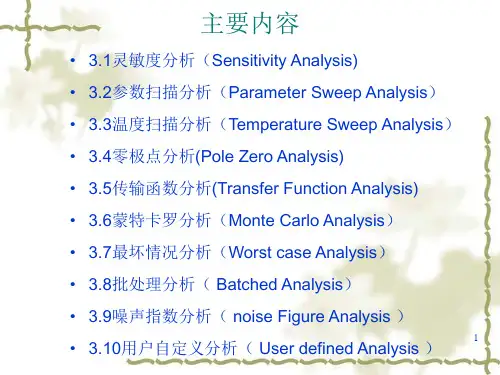
Multisim的电路分析方法：主要有直流工作点分析，交流分析，瞬态分析，傅里叶分析，噪声分析，失真分析，直流扫描分析，灵敏度分析，参数扫描分析，温度扫描分析，零一极点分析，传递函数分析，最坏情况分析，蒙特卡罗分析，批处理分析，用户自定义分析，噪声系数分析。

1.直流工作点分析（DC Operating）:在进行直流工作点分析时，电路中的交流源将被置零，电容开路，电感短路。

2.交流分析（AC Analysis）：交流分析用于分析电路的频率特性。

需先选定被分析的电路节点，在分析时，电路中的直流源将自动置零，交流信号源、电容、电感等均处在交流模式，输入信号也设定为正弦波形式。

若把函数信号发生器的其他信号作为输入激励信号，在进行交流频率分析时，会自动把它作为正弦信号输入。

因此输出响应也是该电路交流频率的函数。

3.瞬态分析（Transient Analysis）：瞬态分析是指定所选定的电路节点的时域响应。

即观察该节点在整个显示周期中每一时刻的电压波形。

在进行瞬态分析时，直流电源保持常数，交流信号源随着时间而改变，电容和电感都是能量储存模式元件。

4.傅里叶分析（Fourier Analysis）：用于分析一个时域信号的直流分量、基频分量和谐波分量。

即把被测节点处的时域变化信号作为离散傅里叶变换，分析的节点，一般将电路中的交流激励源的频率设定为基频，若在电路中有几个交流源时，可以将基频设定在这些频率的最小公因数上。

5.噪声分析（Noise Analysis）:噪声分析用于检查电子线路输出信号的噪声功率幅度，用于计算、分析电阻或晶体管的噪声对电路的影响。

在分析时，假定电路中各自噪声源是互不相关的，因此他们的数值可以分开各自计算。

总的噪声是各自噪声在该节点的和（用有效值表示）。

6.噪声系数分析（Noise Figure Analysis）:主要用于研究元件模型中的噪声参数对电路的影响。

在Multisim中噪声系数定义中：No是输出噪声功率，Ns是信号源电阻的热噪声，G是电路的AC增益（即二端口网络的输出信号与输入信号的比）。

第一部分Multi sim V7原理图编辑，仿真与可编程逻辑入门指导前言祝贺您选择了MultisimV7。

我们有信心将数年来增加的超级设计功能交付给您。

Electronics Workbench是世界领先的电路设计工具供应商，我们的用户比其它任何的EDA开发商的用户都多。

所以我们相信，您将对MultisimV7以及您可能选择的任何其它的Electronics Workbench产品所带来的价值感到满意。

文件惯例当涉及到工具按钮时，相应的工具按钮出现在文字的左边。

虽然multisimV7的电路显示模式是彩色的，但本手册中以黑白模式显示电路。

（您可以将此定制成您喜好的设置）当您看到这样的图标时，所描述的功能只有特定的版本才有。

用户可以购买相应的附加模块。

MultisimV7 用Menu/Item表示菜单命令。

例如，File/|Open表示在File菜单中选择Open命令。

本手册用箭头（ ）表示程序信息。

MultisimV7文件系列MultisimV7文件包括“MultisimV7入门指导”、“User Guide”和在线帮助。

所有的用户都会收到这两本手册的PDF版本。

用户还会收到所购买MultisimV7版本的印刷版手册。

入门指导“入门指导”向您介绍MultisimV7的界面，并指导您学习电路设计（circuit）、仿真（simulate）、分析（analysis）和报告（report）。

User Guide“User Guide”详细介绍了MultisimV7的各项功能，它是基于电路设计层次进行组织的，详细地描述了MultisimV7的各个方面。

在线帮助MultisimV7提供在线帮助文件系统以支持您使用，选择Help|Multisim Help显示包含参考资料（来自于印刷版的附录）的帮助文件，比如对MultisimV7所提供元器件的详细介绍。

所有的帮助文件窗口都是标准窗口，并提供内容列表与索引。

第1章Multisim 7概述随着时代的发展，计算机技术在电子电路设计中发挥着越来越大的作用。

20世纪80年代后期，出现了一批优秀的电子设计自动化（Electronic Design Automation，EDA）软件，如PSPICE、EWB等。

EDA软件工具代表着电子系统设计的技术潮流。

本章介绍加拿大IIT公司（Interactive Image Technologies）具有代表性的EDA软件Multisim 7的特点、安装步骤和用户界面。

1.1 EWB与Multisim 7Electronics Workbench（简称EWB）是加拿大IIT公司于20世纪80年代末推出的电子线路仿真软件。

它可以对模拟、数字和模拟/数字混合电路进行仿真，克服了传统电子产品的设计受实验室客观条件限制的局限性，用虚拟的元件搭建各种电路，用虚拟的仪表进行各种参数和性能指标的测试。

因此，在电子工程设计和高校电子类教学领域中得到广泛应用。

与其他电路仿真软件相比，EWB具有以下特点：1．系统集成度高，界面直观，操作方便EWB软件把电路图的创建、电路的测试分析和仿真结果等内容都集成到一个电路窗口中。

整个操作界面就像一个实验平台。

创建电路所需的元器件、仿真电路所需的测试仪器均可以直接从电路窗口中选取，并且虚拟的元器件、仪器与实物外形非常相似，仪器的操作开关、按键同实际仪器也极为相似。

因此，该软件易学易用。

2．具备模拟、数字及模拟/数字混合电路的仿真在电路窗口中既可以对模拟或数字电路进行仿真，还可以对模拟/数字混合电路进行仿真。

3．提供较为丰富的元器件库EWB的元器件库提供了数千种类型的元器件及各类元器件的理想参数。

用户还可以根据需要修改元件参数或创建新元件。

4．电路分析手段完备EWB除了用7种常用的测试仪表来对仿真电路进行测试之外，还提供了电路的直流工作点分析、瞬态分析、傅里叶分析、噪声分析和失真分析等14种常用的分析方法。

Multi sim V7教学版使用说明书目录目录 (1)第一章前言 (3)1.1 关于本手册 (3)1.2 Multisim V7简介 (3)第二章安装 (6)第三章界面 (8)3.1 MultisimV7界面 (8)3.2 定制MultisimV7界面 (10)第四章元件 (15)4.1 关于本章 (15)4.2 元件工具栏 (15)4.3 操作元件 (16)第五章仪表 (24)5.1 数字万用表 (25)5.2 信号发生器 (26)5.3 示波器 (27)5.4 波特图仪 (29)5.5 IV分析仪 (32)第六章分析方法 06.1 分析方法简介 06.2 静态工作点分析 (3)6.3 交流分析 (5)6.4 瞬态分析 (8)6.5 直流扫瞄分析 (10)6.6 参数扫瞄分析 (12)6.7 传递函数分析 (15)第七章模拟电路仿真步骤 (18)7.1 关于本章 (18)7.2 建立电路 (18)7.3 仿真测量电路 (24)7.4 分析电路 (33)第一章前言1.1 关于本手册本手册针对进行一般模拟电路仿真的MultisimV7用户，概括了MultisimV7单机教学版的安装和主要功能，指导读者逐步地建立一个基本电路，并进行仿真、分析。

本手册所描述的大多数功能，各种版本的MultisimV7都具备。

本手册假定读者已经熟悉了Windows应用，例如，选择菜单命令、用鼠标选择条目以及选中或去选一个选项等。

两个常用名词定义：点击：单击鼠标左键；右击：单击鼠标右键。

1.2 Multisim V7简介随着电子技术和计算机技术的发展，以电子电路计算机辅助设计（Computer Aided Design, 简称CAD）为基础的电子设计自动化（Electronic Design Automation, 简称EDA）技术已成为电子学领域的重要学科。

Multisim 是基于PC平台的电子设计软件，是Electronics Workbench（简称EWB）电路设计软件的升级版本。