Generalized parton distributions of the pion

a r X i v :0712.1947v 2 [h e p -p h ] 24 D e c 2007Generalized Parton Distributions and Nucleon Form FactorsO.V.Selyugin2Momentum transfer dependence of GPDs and pro-ton form factorsOur proposal consists in the attempt tofind a simple ansatz which will be good enough to describe the form factors of the proton and neutron taking into account a number of new data that have appeared in the last years.Let us keep the simple Gaussian ansatz but using some new conditions.To support the proposal[3]and[4]we chose the t-dependence of GPDs in the formH q(x,t)=q(x)exp[a+(1−x)2x bt].(3)with the free parameters b=0.4(determined mostly by the power2of the factor1−x), a±(a+-for H and a−-for E).All these parameters werefixed by analyzing the data on the ratio of proton Pauli and Dirac form-factors.The function q(x)was taken in the same normalization pointµ2=1GeV2as in[6],which is based on the MRST2002global fit[7].In all our calculations we restricted ourselves to the contributions of u and d quarks in H q and E q with E u(x)=k u/N u(1−x)κ1u(x),E d(x)=k dmethod.The other method uses the polarized differential cross section to obtain these form factors.In our model we can obtain the results of both methods by changing the slope of E.So we examined two versions differing by the slopes a−.One can now use the information on the neutron form factors in order to choose the more realistic version.3Neutron form factorsUsing the model developed for proton we can calculate the neutron form factors.For that the isotopic invariance can be used to relate the proton GPDs to the neutron ones,Hence, we do not change any parameters and preserve the same t-dependence of GPDs as in the case of proton.Again,we take two values of the slope a−as in the case of the proton form factors with the same size,which correspond to version(I)and version(II)below.Our calculation of the G n E is shown in Fig.2a.Evidently,thefirst version is in better agreement with experimental data.Therefore, neutron data support the results obtained by polarization transfer method.This conclusion is supported by the calculations of G n M shown in Fig.2b.In this case, it is clearly seen that our parameterization normalized using the proton form-factors ratio from the polarization experiments describes these neutron data quite well.4ConclusionsThe proposed version of Gaussian t-dependence of GPDs reproduces the electromagnetic structure of the proton and neutron sufficiently well.We show that changing only the slope parameters a−of E q it is possible to obtain both the Rosenbluth and Polarization data on the ratio of Pauli and dirac electromagnetic proton form-factors.The description of neutron form-factors is essentially better with the slope parameterfitted to proton polarization transfer data.This is in accordance with the recent theoretical analysis[14].(a)(b)Figure2a.G n E(hard and dot-dashed lines correspond to version(I)and(II));experimental data from[12].Figure2b.G n M(hard and dot-dashed lines correspond to version(I)and(II));experimental data from[13].Acknowledgments We are indebted to M.Anselmino,S.V.Goloskokov,P.Kroll, E.A.Kuraev,E.Predazzi and E.Tomasi-Gustafsson for useful discussions.This work was partially supported by the Deutsche Forschungsgemeinschaft,grant436RUS113/881/0, the Russian Foundation for Basic Research(Grant03-02-16816)and the Russian Feder-ation Ministry of Education and Science(Grant MIREA2.2.2.2.6546). References[1]D.Muller et al.,Fortschr.Phys.42,101(1994);X.Ji,Phys.Rev.Lett.78,610(1998);A.V.Radyushkin,Phys.Rev,D56,5524(1997).[2]M.Burkardt,Phys.Rev.D62,071503(2000).[3]A.V.Radyushkin,Phys.Rev.D58,11400(1998).[4]M.Burkardt,Phys.Lett.B595,245(2004).[5]M.Diehl,Th Feldmann,R.Jakob and P.Kroll,Eur.Phys.J.C39,1(2005).[6]M.Guidal,M.V.Polyakov,A.V.Radyushkin,and M.Vanderhaeghen,Phys.RevD(2005).[7]A.D.Martin et al.,Phys.Lett.B531,216(2002).[8]P.Stoler,Phys.Rev.D65(2002)053013;Phys.Rev.Lett.,91,172303(2003).[9]A.F.Sill et al.,Phys.Rev.D48,29(1993).[10]S.J.Brodsky,hep-ph/0208158.[11]M.K.Jones et al.,Phys.Rev.Lett.,84,1398(2000);O.Gayou et al.,Phys.Rev.C64,038202(2001);O.Gayou et al.,Phys.Rev.Lett.,88,092301(2002);V.Punjabil et al.,Phys.Rev.C71,055202(2005).[12]B.Plaster et al.,Phys.Rev.C73,025205(2006);R.Madey,et al.,Phys.Rev.Lett.91,122002(2003);I.G.Warren,et al.,Phys.Rev.Lett.92,042301(2004).[13]S.Rock,et al.,Phys.Rev.Lett.49,1139(1982).[14]Yu.M.Bystritskiy,E.A.Kuraev and E.Tomasi-Gustafsson,Phys.Rev.C75(2007)015207.。

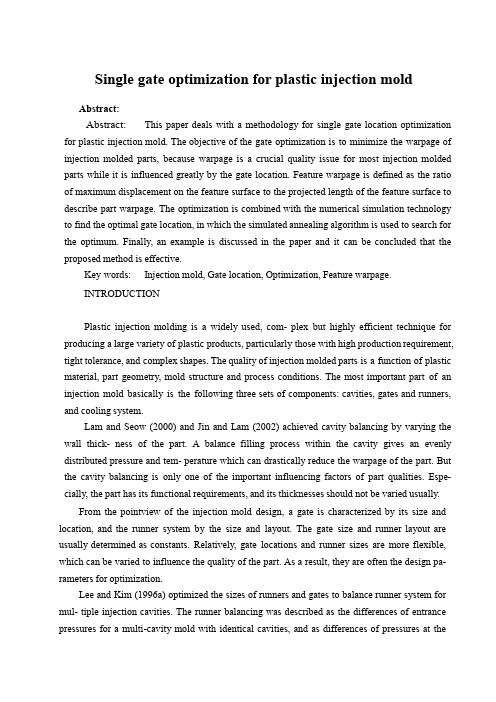
Single gate optimization for plastic injection moldAbstract:Abstract: This paper deals with a methodology for single gate location optimization for plastic injection mold. The objective of the gate optimization is to minimize the warpage of injection molded parts, because warpage is a crucial quality issue for most injection molded parts while it is influenced greatly by the gate location. Feature warpage is defined as the ratio of maximum displacement on the feature surface to the projected length of the feature surface to describe part warpage. The optimization is combined with the numerical simulation technology to find the optimal gate location, in which the simulated annealing algorithm is used to search for the optimum. Finally, an example is discussed in the paper and it can be concluded that the proposed method is effective.Key words: Injection mold, Gate location, Optimization, Feature warpage.INTRODUCTIONPlastic injection molding is a widely used, com- plex but highly efficient technique for producing a large variety of plastic products, particularly those with high production requirement, tight tolerance, and complex shapes. The quality of injection molded parts is a function of plastic material, part geometry, mold structure and process conditions. The most important part of an injection mold basically is the following three sets of components: cavities, gates and runners, and cooling system.Lam and Seow (2000) and Jin and Lam (2002) achieved cavity balancing by varying the wall thick- ness of the part. A balance filling process within the cavity gives an evenly distributed pressure and tem- perature which can drastically reduce the warpage of the part. But the cavity balancing is only one of the important influencing factors of part qualities. Espe- cially, the part has its functional requirements, and its thicknesses should not be varied usually.From the pointview of the injection mold design, a gate is characterized by its size and location, and the runner system by the size and layout. The gate size and runner layout are usually determined as constants. Relatively, gate locations and runner sizes are more flexible, which can be varied to influence the quality of the part. As a result, they are often the design pa- rameters for optimization.Lee and Kim (1996a) optimized the sizes of runners and gates to balance runner system for mul- tiple injection cavities. The runner balancing was described as the differences of entrance pressures for a multi-cavity mold with identical cavities, and as differences of pressures at theend of the melt flow path in each cavity for a family mold with different cavity volumes and geometries. The methodology has shown uniform pressure distributions among the cavities during the entire molding cycle of multiple cavities mold.Zhai et al.(2005a) presented the two gate loca- tion optimization of one molding cavity by an effi- cient search method based on pressure gradient (PGSS), and subsequently positioned weld lines to the desired locations by varying runner sizes for multi-gate parts (Zhai et al., 2006). As large-volume part, multiple gates are needed to shorten the maxi- mum flow path, with a corresponding decrease in injection pressure. The method is promising for de- sign of gates and runners for a single cavity with multiple gates.Many of injection molded parts are produced with one gate, whether in single cavity mold or in multiple cavities mold. Therefore, the gate location of a single gate is the most common design parameter for optimization. A shape analysis approach was pre- sented by Courbebaisse and Garcia (2002), by which the best gate location of injection molding was esti- mated. Subsequently, they developed this methodol- ogy further and applied it to single gate location op- timization of an L shape example (Courbebaisse,2005). It is easy to use and not time-consuming, while it only serves the turning of simple flat parts with uniform thickness.Pandelidis and Zou (1990) presented the opti- mization of gate location, by indirect quality measures relevant to warpage and material degradation, which is represented as weighted sum of a temperature dif- ferential term, an over-pack term, and a frictional overheating term. Warpage is influenced by the above factors, but the relationship between them is not clear. Therefore, the optimization effect is restricted by the determination of the weighting factors.Lee and Kim (1996b) developed an automated selection method of gate location, in which a set of initial gate locations were proposed by a designer and then the optimal gate was located by the adjacent node evaluation method. The conclusion to a great extent depends much on the human design er’s in tuition, because the first step of the method is based on the desi gner’s proposition. So the result is to a large ex- tent limited to the designer’s experience.Lam and Jin (2001) developed a gate location optimization method based on the minimization of the Standard Deviation of Flow Path Length (SD[L]) and Standard Deviation of Filling Time (SD[T]) during the molding filling process. Subsequently, Shen et al.(2004a; 2004b) optimized the gate location design by minimizing the weighted sum of filling pressure, filling time difference between different flow paths, temperature difference, and over-pack percentage. Zhai et al.(2005b) investigated optimal gate location with evaluation criteria of injection pressure at the end of filling. These researchers presented the objec- tive functions asperformances of injection molding filling operation, which are correlated with product qualities. But the correlation between the perform- ances and qualities is very complicated and no clear relationship has been observed between them yet. It is also difficult to select appropriate weighting factors for each term.A new objective function is presented here to evaluate the warpage of injection molded parts to optimize gate location. To measure part quality di- rectly, this investigation defines feature warpage to evaluate part warpage, which is evaluated from the “flow plus warpage” simulation outputs of Moldflow Plastics Insight (MPI) software. The objective func- tion is minimized to achieve minimum deformation in gate location optimization. Simulated annealing al- gorithm is employed to search for the optimal gate location. An example is given to illustrate the effec- tivity of the proposed optimization procedure.QUALITY MEASURES: FEATURE WARPGEDefinition of feature warp ageTo apply optimization theory to the gate design, quality measures of the part must be specified in the first instance. The term “quality” may be referred to many product properties, such as mechanical, thermal, electrical, optical, ergonomical or geometrical prop- erties. There are two types of part quality measures: direct and indirect. A model that predicts the proper- ties from numerical simulation results would be characterized as a direct quality measure. In contrast, an indirect measure of part quality is correlated with target quality, but it cannot provide a direct estimate of that quality.For warpage, the indirect quality measures in related works are one of performances of injection molding flowing behavior or weighted sum of those. The performances are presented as filling time dif- ferential along different flow paths, temperature dif- ferential, over-pack percentage, and so on. It is ob- vious that warpage is influenced by these perform- ances, but the relationship between warpage and these performances is not clear and the determination of these weighting factors is rather difficult. Therefore, the optimization with the above objective function probably will not minimize part warpage even with perfect optimization technique. Sometimes, improper weighting factors will result in absolutely wrong re- sults.Some statistical quantities calculated from the nodal displacements were characterized as direct quality measures to achieve minimum deformation in related optimization studies. The statistical quantities are usually a maximum nodal displacement, an av- erage of top 10 percentile nodal displacements, and an overall average nodal displacement (Lee and Kim,1995; 1996b). These nodal displacements are easy to obtain from the simulation results, the statistical val- ues, to some extents, representing the deformation. But the statistical displacement cannot effectively describe the deformation of the injection molded parts.In industry, designers and manufacturers usually pay more attention to the degree of part warpage on some specific features than the whole deformation of the injection molded parts. In this study, feature warpage is defined to describe the deformation of the injection parts. The feature warpage is the ratio of the maximum displacement of the feature surface to the projected length of the feature surface (Fig.1):where γ is the feature warpage, h is the maximum displacement on the feature surface deviating from the reference platform, and L is the projected length of the feature surface on a reference direction paralleling the reference platform.For complicated features (only plane feature discussed here), the feature warpage is usually sepa- rated into two constituents on the reference plane, which are represented on a 2D coordinate system:where γx, γy are the constituent feature warpages in the X, Y direction, and L x, L y are the projected lengths of the feature surface on X, Y component.Evaluation of feature wa rpageAfter the determination of target feature com- bined with corresponding reference plane and pro- jection direction, the value of L can be calculated immediately from the part with the calculating method of analytic geometry (Fig.2). L is a constant for any part on the specified feature surface and pro- jected direction. But the evaluation of h is more com- plicated than that of L.Simulation of injection molding process is a common technique to forecast the quality of part de- sign, mold design and process settings. The results of warpage simulation are expressed as the nodal de- flections on X, Y, Z component (W x, W y, W z), and the nodal displacement W. W is the vector length of vector sum of W x·i, W y·j, and W z·k, where i, j, k are the unit vectors on X, Y, Z component. The h is the maximum displacement of the nodes on the feature surface, which is correlated with the normal orientation of the reference plane, and can be derived from the results of warpage simulation.To calculate h, the deflection of ith node is evaluated firstly as follows:where W i is the deflection in the normal direction of the reference plane of ith node; W ix, W iy, W iz are the deflections on X, Y, Z component of ith node; α,β,γ are the angles of normal vector of the reference; A and B are the terminal nodes of the feature to projectingdirection (Fig.2); WA and WB are the deflections of nodes A and B:where W Ax, W Ay, W Az are the deflections on X, Y, Zcomponent of node A; W Bx, W By and W Bz are the de- flections on X, Y, Z component of node B; ωiA and ωiB are the weighting factors of the terminal node deflections calculated as follows:where L iA is the projector distance between ith node and node A. Ultimately, h is the maximum of the absolute value of W i:In industry, the inspection of the warpage is carried out with the help of a feeler gauge, while the measured part should be placed on a reference plat- form. The value of h is the maximum numerical reading of the space between the measured part sur- face and the reference platform.GATE LOCATION OPTIMIZATION PROBLEM FORMATIONThe quality term “warpag e”means the perma- nent deformation of the part, which is not caused by an applied load. It is caused by differential shrinkage throughout the part, due to the imbalance of polymer flow, packing, cooling, and crystallization.The placement of a gate in an injection mold is one of the most important variables of the total mold design. The quality of the molded part is greatly af- fected by the gate location, because it influences the manner that the plastic flows into the mold cavity. Therefore, different gate locations introduce inho- mogeneity in orientation, density, pressure, and temperature distribution, accordingly introducing different value and distribution of warpage. Therefore, gate location is a valuable design variable to minimize the injection molded part warpage. Because the cor- relation between gate location and warpage distribu- tion is to a large extent independent of the melt and mold temperature, it is assumed that the moldingconditions are kept constant in this investigation. The injection molded part warpage is quantified by the feature warpage which was discussed in the previous section.The single gate location optimization can thus be formulated as follows:Minimize:Subject to:where γ is the feature warpage; p is the injection pressure at the gate position; p0 is the allowable in- jection pressure of injection molding machine or the allowable injection pressure specified by the designer or manufacturer; X is the coordinate vector of the candidate gate locations; X i is the node on the finite element mesh model of the part for injection molding process simulation; N is the total number of nodes.In the finite element mesh model of the part, every node is a possible candidate for a gate. There- fore, the total number of the possible gate location N p is a function of the total number of nodes N and the total number of gate locations to be optimized n:In this study, only the single-gate location problem is investigated.SIMULATED ANNEALING ALGORITHMThe simulated annealing algorithm is one of the most powerful and popular meta-heuristics to solve optimization problems because of the provision of good global solutions to real-world problems. The algorithm is based upon that of Metropolis et al. (1953), which was originally proposed as a means to find an equilibrium configuration of a collection of atoms at a given temperature. The connection be- tween this algorithm and mathematical minimization was first noted by Pincus (1970), but it was Kirkpatrick et al.(1983) who proposed that it formed the basis of an optimization technique for combina- tional (and other) problems.To apply the simulated annealing method to op timization problems, the objective function f is used as an energy function E. Instead of finding a low energy configuration, the problem becomes to seek an approximate global optimal solution. The configura- tions of the values of design variables are substituted for the energy configurations of the body, and the control parameter for the process is substituted for temperature. A random number generator is used as a way of generating new values for the design variables. It is obvious that this algorithm just takes the mini- mization problems into account. Hence, while per- forming a maximization problem the objective func- tion is multiplied by (−1) to obtain a capable form.The major advantage of simulated annealing algorithm over other methods is the ability to avoid being trapped at local minima. This algorithm em- ploys a random search, which not only accepts changes that decrease objective function f, but also accepts some changes that increase it. The latter are accepted with a probability pwhere ∆f is the increase of f, k is Boltzm an’s constant, and T is a control parameter which by analogy with the original application is known as the system “tem perature”irrespective of the objective function involved.In the case of gate location optimization, the implementation of this algorithm is illustrated in Fig.3, and this algorithm is detailed as follows:(1) SA algorithm starts from an initial gate loca- tion X old with an assigned value T k of the “tempera- ture”parameter T (the “temperature” counter k is initially set to zero). Proper control parameter c (0<c<1) in annealing process and Markov chain N generateare given.(2) SA algorithm generates a new gate location X new in the neighborhood of X old and the value of the objective function f(X) is calculated.(3) The new gate location will be accepted with probability determined by the acceptance functionFig.3 The flow chart of the simulated annealing algorithmAPPLICATION AND DISCUSSIONThe application to a complex industrial part is presented in this section to illustrate the proposed quality measure and optimization methodology. The part is provided by a manufacturer, as shown in Fig.4. In this part, the flatness of basal surface is the most important profileprecision requirement. Therefore, the feature warpage is discussed on basal surface, in which reference platform is specified as a horizontal plane attached to the basal surface, and the longitu- dinal direction is specified as projected reference direction. The parameter h is the maximum basal surface deflection on the normal direction, namely the vertical direction, and the parameter L is the projected length of the basal surface to the longitudinal direc- tion.Fig.4 Industrial part provided by the manufac tur e rThe material of the part is Nylon Zytel 101L (30% EGF, DuPont Engineering Polymer). The molding conditions in the simulation are listed in T able 1. Fig.5 shows the finite element mesh model ofthe part employed in the numerical simulation. It has1469 nodes and 2492 elements. The objective func- tion, namely feature warpage, is evaluated by Eqs.(1), (3)~(6). The h is evaluated from the results of “Flow+Warp” Analysis Sequence in MPI by Eq.(1), and the L is measured on the industrial part immediately, L=20.50 mm.MPI is the most extensive software for the in- jection molding simulation, which can recommend the best gate location based on balanced flow. Gate location analysis is an effective tool for gate location design besides empirical method. For this part, the gate location analysis of MPI recommends that the best gate location is near node N7459, as shown in Fig.5. The part warpage is simulated based on this recommended gate and thus the feature warpage is evaluated: γ=5.15%, which is a great value. In trial manufacturing, part warpage is visible on the sample work piece. This is unacceptable for the manufacturer.The great warpage on basal surface is caused bythe uneven orientation distribution of the glass fiber, as shown in Fig.6a. Fig.6a shows that the glass fiber orientation changes from negative direction to posi- tive direction because of the location of the gate, par- ticularly thegreatest change of the fiber orientation appears near the gate. The great diversification of fiber orientation caused by gate location introduces serious differential shrinkage. Accordingly, the fea- ture warpage is notable and the gate location must be optimized to reduce part warpageT o optimize the gate location, the simulated an- nealing searching discussed in the section “Simulated annealing algorithm” is applied to this part. The maximum number of iterations is chosen as 30 to ensure the precision of the optimization, and the maximum number of random trials allowed for each iteration is chosen as 10 to decrease the probability of null iteration without an iterative solution. Node N7379 (Fig.5) is found to be the optimum gate loca- tion.The feature warpage is evaluated from the war- page simulation results f(X)=γ=0.97%, which is less than that of the recommended gate by MPI. And the part warpage meets the manufacturer’s requirements in trial manufacturing. Fig.6b shows the fiber orien- tation in the simulation. It is seen that the optimal gate location results in the even glass fiber orientation, and thus introduces great reduction of shrinkage differ- ence on the vertical direction along the longitudinal direction. Accordingly, the feature warpage is re- duced.CONCLUSIONFeature warpage is defined to describe the war- page of injection molded parts and is evaluated based on the numerical simulation software MPI in this investigation. The feature warpage evaluation based on numerical simulation is combined with simulated annealing algorithm to optimize the single gate loca- tion for plastic injection mold. An industrial part is taken as an example to illustrate the proposed method. The method results in an optimal gate location, by which the part is satisfactory for the manufacturer. This method is also suitable to other optimization problems for warpage minimization, such as location optimization for multiple gates, runner system bal- ancing, and option of anisotropic materials.注塑模的单浇口优化摘要：本文论述了一种单浇口位置优化注塑模具的方法。

distribution的用法Distribution是英语中一个常用的词汇，它可以表示分配、分发、分布等含义。

在不同的语境下，我们可以使用不同的表达方式和搭配，来描述Distribution的不同用法和含义。

1. Distribution作为名词，表示分配、分发、分布。

例如：- The distribution of resources is a key factor in economic development.（资源的分配是经济发展的关键因素。

）- The distribution of flyers was completed ahead of schedule.（传单的分发提前完成了。

）- The distribution of wealth is highly unequal in many countries.（在许多国家，财富分配极不平等。

）2. Distribution作为动词，表示分配、分发。

例如：- The manager is responsible for distributing the workload among the team members.（经理负责将工作负担分配给团队成员。

） - The charity organization distributed food and clothing to the needy families.（慈善组织向需要帮助的家庭分发食品和衣物。

）3. Distribution还可以作为数学和统计学中的专业术语，表示概率分布、频率分布等。

例如：- The distribution of the sample data can be used to estimate the population parameters.（样本数据的分布可以用来估计总体参数。

）- The normal distribution is widely used in statistical analysis.（正态分布在统计分析中被广泛应用。

normal distributionnormal distribution, also called gaussian distribution, the most mon distribution function for independent, randomly generated variables. its familiar bell-shaped curve is ubiquitous in statistical reports, fromsurvey analysis and quality control to resource allocation.the graph of the normal distribution is characterized by two parameters: the mean, or average, which is the maximum of the graph and about which the graph is always symmetric; and the standard deviation, which determines the amount of dispersion away from the mean.a small standard deviation (pared with the mean) produces a steep graph, whereas a large standard deviation (again pared with the mean) produces a flat graph. see the figure.the normal distribution is produced by the normal density function, p(x) = e−(x−μ)2/2σ2/σsquare rootof√2π. in this exponential function e is the constant 2.71828…, is the mean, and σ is the standard deviation. the probability of a random variablefalling within any given range of values is equal to the proportion of the area enclosed under thefunction’s graph between the given values and above the x-axis. because the denominator (σsquare rootof√2π), known as the normalizing coefficient, causes the total area enclosed by the graph to be exactly equal to unity, probabilities can be obtained directlyfrom the corresponding area—i.e., an area of 0.5 corresponds to a probability of 0.5. although these areas can be determined with calculus, tables were generated in the 19th century for the special caseof = 0 and σ= 1, known as the standard normal distribution, and these tables can be used for any normal distribution after the variables are suitably rescaled by subtracting their mean and dividing by their standard deviation, (x−μ)/σ. calculators have now all but eliminated the use of such tables.for further details see probability theory.the term “gaussian distribution” refers to the german mathematician carl friedrich gauss, who first developed a two-parameter exponential function in 1809 in connection with studies of astronomical observation errors. this study led gauss to formulate his law of observational error and to advance the theory of the method of least squares approximation. another famous early application of the normal distribution was by the british physicist james clerk maxwell, who in 1859 formulated his law of distribution of molecular velocities—later generalized as the maxwell-boltzmann distribution law.the french mathematician abraham de moivre, in his doctrine of chances (1718), first noted that probabilities associated with discretely generated random variables (such as are obtained by flipping a coin or rolling a die) can be approximated by the area under the graph of an exponential function. thisresult was extended and generalized by the frenchscientist pierre-simon laplace, in his théorie analytique des probabilités(1812; “analytic theory of probability”), into the first central limit theorem, which proved that probabilities for almostall independent and identically distributed random variables converge rapidly (with sample size) to the area under an exponential function—that is, to a normal distribution. the central limit theorem permitted hitherto intractable problems, particularly those involving discrete variables, to be handled with calculus.。

CH7Nonrandom Sampling - Every unit of the population does not have the same probability of being included in the sampleRandom sampling - Every unit of the population has the same probability of being included in the sample.Random Sampling TechniquesSimple Random Sample – basis for other random sampling techniques Stratified Random SampleProportionate -- the percentage of the sample taken from each stratum is proportionate to the percentage that each stratum(層) is within the populationDisproportionate -- proportions of the strata within the sample are different than the proportions of the strata within the populationPopulation is divided into non-overlapping subpopulations called strata Researcher extracts a simple random sample from each subpopulation Stratified random sampling has the potential for reducing error Sampling error – a sample does not represent the populationStratified random sampling has the potential to match the sample closely to the population Stratified sampling is more costlyStratum should be relatively homogeneous, i.e. race, gender, religion Systematic Random SamplePopulation elements are an ordered sequence.With systematic sampling, every k th item is selected to produce a sample of size n from a population of size NSystematic sampling is evenly distributed across the frame Sample elements are selected at a constant interval, k, from the ordered sequence frame.Systematic sampling is based on the assumption that the source of the population is random Cluster (or Area) SamplingCluster sampling – involves dividing the population into non-overlapping areas Identifies the clusters that tend to be internally homogeneous Each cluster is a microcosm(縮圖) of the populationIf the cluster is too large, a second set of clusters is taken from each original cluster This is two stage samplingAdvantagesMore convenient for geographically dispersed populations Simplified administration of the surveyUnavailability of sampling frame prohibits using other random sampling methodsn =sample size N=population size k =size of selection intervalk =N nDisadvantagesStatistically less efficient when the cluster elements are similarCosts and problems of statistical analysis are greater than for simple random samplingNon-Random sampling – sampling techniques used to select elements from the population by any mechanism that does not involve a random selection processErrors:Data from nonrandom samples are not appropriate for analysis by inferential statistical methods.Sampling Error occurs when the sample is not representative of the populationNon-sampling Errors – all errors other than sampling errorsMissing Data, Recording, Data Entry, and Analysis ErrorsPoorly conceived concepts , unclear definitions, and defective questionnairesResponse errors occur when people do not know, will not say, or overstate in their answersCentral Limit Theorem(中央極限定理)Central limits theorem allows one to study populations with differently shaped distributionsCentral limits theorem creates the potential for applying the normal distribution to many problems when sample size is sufficiently largeAdvantage of Central Limits theorem is when sample data is drawn from populations not normally distributed or populations of unknown shape can also be analyzed because the sample means are normally distributed due to large sample sizesAs sample size increases, the distribution narrowsDue to the Std Dev of the meanStd Dev of mean decreases as sample size increasesZ Formula for Sample MeansSampling Distribution of PSample ProportionSampling DistributionnQ > 5 (P is the population proportion and Q = 1 - P.)The mean of the distribution is P.The standard deviation of the distribution is Z Formula for Sample Proportions.deviationstandardandmeanon withdistributinormalaisxofondistributithe,ofdeviationstandardandofmeanwithpopulationnormalafromnsizeofsamplerandomaofmeantheisxIfxxnσμσμσμ== nXXZX Xσμσμ-=-=P = Xn√(p∗q)/n。

统计学中英文对照表2008—03—21 11:39Absolutedeviation,绝对离差Absolutenumber,绝对数Absoluteresiduals，绝对残差Accelerationarray，加速度立体阵Accelerationinanarbitrarydirection,任意方向上的加速度Accelerationnormal,法向加速度Accelerationspacedimension，加速度空间的维数Accelerationtangential,切向加速度Accelerationvector，加速度向量Acceptablehypothesis,可接受假设Accumulation,累积Accuracy,准确度Actualfrequency，实际频数Adaptiveestimator,自适应估计量Addition,相加Additiontheorem，加法定理Additivity，可加性Adjustedrate,调整率Adjustedvalue，校正值Admissibleerror,容许误差Aggregation,聚集性Alternativehypothesis,备择假设Amonggroups，组间Amounts,总量Analysisofcorrelation，相关分析Analysisofcovariance，协方差分析Analysisofregression，回归分析Analysisoftimeseries,时间序列分析Analysisofvariance,方差分析Angulartransformation,角转换ANOVA（analysisofvariance）,方差分析ANOVAModels,方差分析模型Arcing，弧/弧旋Arcsinetransformation，反正弦变换Areaunderthecurve，曲线面积AREG，评估从一个时间点到下一个时间点回归相关时的误差ARIMA，季节和非季节性单变量模型的极大似然估计Arithmeticgridpaper，算术格纸Arithmeticmean,算术平均数Arrheniusrelation，艾恩尼斯关系Assessingfit，拟合的评估Associativelaws，结合律Asymmetricdistribution,非对称分布Asymptoticbias,渐近偏倚Asymptoticefficiency，渐近效率Asymptoticvariance,渐近方差Attributablerisk，归因危险度Attributedata,属性资料Attribution,属性Autocorrelation，自相关Autocorrelationofresiduals，残差的自相关Average，平均数Averageconfidenceintervallength，平均置信区间长度Averagegrowthrate，平均增长率Barchart,条形图Bargraph,条形图Baseperiod,基期Bayes’theorem，Bayes定理Bell-shapedcurve，钟形曲线Bernoullidistribution，伯努力分布Best-trimestimator，最好切尾估计量Bias,偏性Binarylogisticregression,二元逻辑斯蒂回归Binomialdistribution，二项分布Bisquare，双平方BivariateCorrelate，二变量相关Bivariatenormaldistribution，双变量正态分布Bivariatenormalpopulation，双变量正态总体Biweightinterval,双权区间BiweightM—estimator,双权M估计量Block，区组/配伍组BMDP(Biomedicalcomputerprograms）,BMDP统计软件包Boxplots，箱线图/箱尾图Breakdownbound,崩溃界/崩溃点Canonicalcorrelation,典型相关Caption，纵标目Case—controlstudy，病例对照研究Categoricalvariable,分类变量Catenary,悬链线Cauchydistribution,柯西分布Cause-and—effectrelationship,因果关系Cell,单元Censoring,终检Centerofsymmetry,对称中心Centeringandscaling,中心化和定标Centraltendency,集中趋势Centralvalue，中心值CHAID—χ2AutomaticInteractionDetector，卡方自动交互检测Chance，机遇Chanceerror,随机误差Chancevariable，随机变量Characteristicequation,特征方程Characteristicroot，特征根Characteristicvector，特征向量Chebshevcriterionoffit,拟合的切比雪夫准则Chernofffaces，切尔诺夫脸谱图Chi—squaretest，卡方检验/χ2检验Choleskeydecomposition,乔洛斯基分解Circlechart，圆图Classinterval，组距Classmid—value,组中值Classupperlimit,组上限Classifiedvariable,分类变量Clusteranalysis，聚类分析Clustersampling,整群抽样Code，代码Codeddata，编码数据Coding，编码Coefficientofcontingency,列联系数Coefficientofdetermination，决定系数Coefficientofmultiplecorrelation，多重相关系数Coefficientofpartialcorrelation,偏相关系数Coefficientofproduction-momentcorrelation,积差相关系数Coefficientofrankcorrelation，等级相关系数Coefficientofregression，回归系数Coefficientofskewness,偏度系数Coefficientofvariation,变异系数Cohortstudy，队列研究Column，列Columneffect，列效应Columnfactor,列因素Combinationpool,合并Combinativetable,组合表Commonfactor,共性因子Commonregressioncoefficient,公共回归系数Commonvalue，共同值Commonvariance,公共方差Commonvariation，公共变异Communalityvariance,共性方差Comparability，可比性Comparisonofbathes,批比较Comparisonvalue,比较值Compartmen**＊el，分部模型Compassion，伸缩Complementofanevent，补事件Completeassociation，完全正相关Completedissociation,完全不相关Completestatistics,完备统计量Completelyrandomizeddesign，完全随机化设计Compositeevent,联合事件Compositeevents，复合事件Concavity，凹性Conditionalexpectation，条件期望Conditionallikelihood，条件似然Conditionalprobability,条件概率Conditionallylinear，依条件线性Confidenceinterval，置信区间Confidencelimit,置信限Confidencelowerlimit,置信下限Confidenceupperlimit，置信上限ConfirmatoryFactorAnalysis，验证性因子分析Confirmatoryresearch,证实性实验研究Confoundingfactor,混杂因素Conjoint，联合分析Consistency,相合性Consistencycheck,一致性检验Consistentasymptoticallynormalestimate,相合渐近正态估计Consistentestimate，相合估计Constrainednonlinearregression，受约束非线性回归Constraint，约束Contaminateddistribution,污染分布ContaminatedGausssian，污染高斯分布Contaminatednormaldistribution,污染正态分布Contamination，污染Contaminationmodel，污染模型Contingencytable,列联表Contour，边界线Contributionrate,贡献率Control，对照Controlledexperiments，对照实验Conventionaldepth,常规深度Convolution，卷积Correctedfactor,校正因子Correctedmean,校正均值Correctioncoefficient，校正系数Correctness，正确性Correlationcoefficient,相关系数Correlationindex,相关指数Correspondence，对应Counting,计数Counts，计数/频数Covariance，协方差Covariant，共变CoxRegression,Cox回归Criteriaforfitting,拟合准则Criteriaofleastsquares,最小二乘准则Criticalratio，临界比Criticalregion,拒绝域Criticalvalue,临界值Cross-overdesign,交叉设计Cross-sectionanalysis，横断面分析Cross-sectionsurvey，横断面调查Crosstabs，交叉表Cross—tabulationtable,复合表Cuberoot，立方根Cumulativedistributionfunction,分布函数Cumulativeprobability,累计概率Curvature,曲率/弯曲Curvature，曲率Curvefit，曲线拟和Curvefitting,曲线拟合Curvilinearregression,曲线回归Curvilinearrelation，曲线关系Cut-and-trymethod，尝试法Cycle，周期Cyclist，周期性Dtest，D检验Dataacquisition，资料收集Databank，数据库Datacapacity，数据容量Datadeficiencies,数据缺乏Datahandling,数据处理Datamanipulation，数据处理Dataprocessing，数据处理Datareduction，数据缩减Dataset,数据集Datasources，数据来源Datatransformation，数据变换Datavalidity，数据有效性Data—in，数据输入Data—out，数据输出Deadtime,停滞期Degreeoffreedom，自由度Degreeofprecision，精密度Degreeofreliability，可靠性程度Degression,递减Densityfunction,密度函数Densityofdatapoints，数据点的密度Dependentvariable,应变量/依变量/因变量Dependentvariable,因变量Depth,深度Derivativematrix，导数矩阵Derivative-freemethods，无导数方法Design,设计Determinacy，确定性Determinant，行列式Determinant,决定因素Deviation,离差Deviationfromaverage,离均差Diagnosticplot，诊断图Dichotomousvariable,二分变量Differentialequation,微分方程Directstandardization,直接标准化法Discretevariable，离散型变量DISCRIMINANT，判断Discriminantanalysis，判别分析Discriminantcoefficient，判别系数Discriminantfunction，判别值Dispersion,散布/分散度Disproportional，不成比例的Disproportionatesub-classnumbers,不成比例次级组含量Distributionfree,分布无关性/免分布Distributionshape，分布形状Distribution-freemethod,任意分布法Distributivelaws,分配律Disturbance,随机扰动项Doseresponsecurve，剂量反应曲线Doubleblindmethod,双盲法Doubleblindtrial,双盲试验Doubleexponentialdistribution,双指数分布Doublelogarithmic,双对数Downwardrank,降秩Dual-spaceplot,对偶空间图DUD，无导数方法Duncan'snewmultiplerangemethod,新复极差法/Duncan新法Effect，实验效应Eigenvalue，特征值Eigenvector,特征向量Ellipse，椭圆Empiricaldistribution，经验分布Empiricalprobability，经验概率单位Enumerationdata，计数资料Equalsun—classnumber，相等次级组含量Equallylikely,等可能Equivariance,同变性Error，误差/错误Errorofestimate,估计误差ErrortypeI，第一类错误ErrortypeII,第二类错误Es＊＊＊,被估量Estimatederrormeansquares,估计误差均方Estimatederrorsumofsquares,估计误差平方和Euclideandistance，欧式距离Event,事件Event，事件Exceptionaldatapoint，异常数据点Expectationplane，期望平面Expectationsurface,期望曲面Expectedvalues，期望值Experiment,实验Experimentalsampling,试验抽样Experimentalunit,试验单位Explanatoryvariable,说明变量Exploratorydataanalysis,探索性数据分析ExploreSummarize，探索—摘要Exponentialcurve,指数曲线Exponentialgrowth,指数式增长EXSMOOTH，指数平滑方法Extendedfit,扩充拟合Extraparameter,附加参数Extrapolation，外推法Extremeobservation，末端观测值Extremes，极端值/极值Fdistribution，F分布Ftest,F检验Factor,因素/因子Factoranalysis，因子分析FactorAnalysis，因子分析Factorscore，因子得分Factorial，阶乘Factorialdesign,析因试验设计Falsenegative,假阴性Falsenegativeerror，假阴性错误Familyofdistributions,分布族Familyofestimators，估计量族Fanning，扇面Fatalityrate，病死率Fieldinvestigation,现场调查Fieldsurvey，现场调查Finitepopulation，有限总体Finite—sample，有限样本Firstderivative,一阶导数Firstprincipalcomponent，第一主成分Firstquartile，第一四分位数Fisherinformation,费雪信息量Fittedvalue,拟合值Fittingacurve,曲线拟合Fixedbase，定基Fluctuation，随机起伏Forecast，预测Fourfoldtable,四格表Fourth，四分点Fractionblow，左侧比率Fractionalerror,相对误差Frequency，频率Frequencypolygon,频数多边图Frontierpoint,界限点Functionrelationship,泛函关系Gammadistribution，伽玛分布Gaussincrement,高斯增量Gaussiandistribution，高斯分布/正态分布Gauss—Newtonincrement,高斯-牛顿增量Generalcensus,全面普查GENLOG(Generalizedlinermodels)，广义线性模型Geometricmean,几何平均数Gini’smeandifference，基尼均差GLM(Generallinermodels）,通用线性模型Goodnessoffit,拟和优度/配合度Gradientofdeterminant,行列式的梯度Graeco-Latinsquare,希腊拉丁方Grandmean,总均值Grosserrors，重大错误Gross—errorsensitivity，大错敏感度Groupaverages,分组平均Groupeddata,分组资料Guessedmean，假定平均数Half—life，半衰期HampelM-estimators，汉佩尔M估计量Happenstance，偶然事件Harmonicmean，调和均数Hazardfunction，风险均数Hazardrate,风险率Heading,标目Heavy—taileddistribution，重尾分布Hessianarray，海森立体阵Heterogeneity,不同质Heterogeneityofvariance,方差不齐Hierarchicalclassification,组内分组Hierarchicalclusteringmethod,系统聚类法High—leveragepoint，高杠杆率点HILOGLINEAR，多维列联表的层次对数线性模型Hinge,折叶点Histogram,直方图Historicalcohortstudy，历史性队列研究Holes，空洞HOMALS,多重响应分析Homogeneityofvariance,方差齐性Homogeneitytest,齐性检验HuberM-estimators,休伯M估计量Hyperbola,双曲线Hypothesistesting，假设检验Hypotheticaluniverse,假设总体Impossibleevent，不可能事件Independence，独立性Independentvariable,自变量Index,指标/指数Indirectstandardization，间接标准化法Individual,个体Inferenceband，推断带Infinitepopulation,无限总体Infinitelygreat,无穷大Infinitelysmall，无穷小Influencecurve,影响曲线Informationcapacity，信息容量Initialcondition,初始条件Initialestimate,初始估计值Initiallevel,最初水平Interaction，交互作用Interactionterms，交互作用项Intercept,截距Interpolation,内插法Interquartilerange，四分位距Intervalestimation，区间估计Intervalsofequalprobability，等概率区间Intrinsiccurvature,固有曲率Invariance,不变性Inversematrix,逆矩阵Inverseprobability，逆概率Inversesinetransformation，反正弦变换Iteration,迭代Jacobiandeterminant,雅可比行列式Jointdistributionfunction，分布函数Jointprobability，联合概率Jointprobabilitydistribution,联合概率分布Kmeansmethod,逐步聚类法Kaplan—Meier，评估事件的时间长度Kaplan—Merierchart,Kaplan-Merier图Kendall'srankcorrelation，Kendall等级相关Kinetic，动力学Kolmogorov—Smirnovetest，柯尔莫哥洛夫-斯米尔诺夫检验KruskalandWallistest，Kruskal及Wallis检验/多样本的秩和检验/H检验Kurtosis，峰度Lackoffit，失拟Ladderofpowers,幂阶梯Lag,滞后Largesample，大样本Largesampletest,大样本检验Latinsquare，拉丁方Latinsquaredesign，拉丁方设计Leakage,泄漏Leastfavorableconfiguration,最不利构形Leastfavorabledistribution,最不利分布Leastsignificantdifference，最小显著差法Leastsquaremethod，最小二乘法Least-absolute-residualsestimates，最小绝对残差估计Least-absolute-residualsfit，最小绝对残差拟合Least—absolute—residualsline,最小绝对残差线Legend，图例L—estimator,L估计量L-estimatoroflocation，位置L估计量L—estimatorofscale，尺度L估计量Level，水平Lifeexpectance,预期期望寿命Lifetable，寿命表Lifetablemethod，生命表法Light—taileddistribution，轻尾分布Likelihoodfunction，似然函数Likelihoodratio，似然比linegraph,线图Linearcorrelation，直线相关Linearequation，线性方程Linearprogramming,线性规划Linearregression,直线回归LinearRegression,线性回归Lineartrend，线性趋势Loading,载荷Locationandscaleequivariance，位置尺度同变性Locationequivariance,位置同变性Locationinvariance,位置不变性Locationscalefamily,位置尺度族Logranktest，时序检验Logarithmiccurve，对数曲线Logarithmicnormaldistribution，对数正态分布Logarithmicscale,对数尺度Logarithmictransformation,对数变换Logiccheck,逻辑检查Logisticdistribution，逻辑斯特分布Logittransformation,Logit转换LOGLINEAR，多维列联表通用模型Lognormaldistribution，对数正态分布Lostfunction，损失函数Lowcorrelation，低度相关Lowerlimit，下限Lowest—attainedvariance，最小可达方差LSD,最小显著差法的简称Lurkingvariable,潜在变量Main effect，主效应Major heading，主辞标目Marginal density function,边缘密度函数Marginal probability，边缘概率Marginal probability distribution,边缘概率分布Matched data，配对资料Matched distribution，匹配过分布Matching of distribution，分布的匹配Matching of transformation,变换的匹配Mathematical expectation,数学期望Mathematical model，数学模型Maximum L—estimator,极大极小L 估计量Maximum likelihood method,最大似然法Mean，均数Mean squares between groups,组间均方Mean squares within group，组内均方Means （Compare means），均值-均值比较Median,中位数Median effective dose，半数效量Median lethal dose,半数致死量Median polish，中位数平滑Median test，中位数检验Minimal sufficient statistic,最小充分统计量Minimum distance estimation，最小距离估计Minimum effective dose，最小有效量Minimum lethal dose，最小致死量Minimum variance estimator,最小方差估计量MINITAB,统计软件包Minor heading，宾词标目Missing data，缺失值Model specification,模型的确定Modeling Statistics ，模型统计Models for outliers，离群值模型Modifying the model,模型的修正Modulus of continuity，连续性模Morbidity,发病率Most favorable configuration,最有利构形Multidimensional Scaling （ASCAL),多维尺度/多维标度Multinomial Logistic Regression ，多项逻辑斯蒂回归Multiple comparison，多重比较Multiple correlation ，复相关Multiple covariance,多元协方差Multiple linear regression,多元线性回归Multiple response ,多重选项Multiple solutions，多解Multiplication theorem,乘法定理Multiresponse，多元响应Multi-stage sampling,多阶段抽样Multivariate T distribution,多元T分布Mutual exclusive,互不相容Mutual independence，互相独立Natural boundary，自然边界Natural dead,自然死亡Natural zero，自然零Negative correlation，负相关Negative linear correlation,负线性相关Negatively skewed，负偏Newman-Keuls method,q检验NK method,q检验No statistical significance,无统计意义Nominal variable,名义变量Nonconstancy of variability,变异的非定常性Nonlinear regression，非线性相关Nonparametric statistics,非参数统计Nonparametric test,非参数检验Nonparametric tests，非参数检验Normal deviate,正态离差Normal distribution,正态分布Normal equation，正规方程组Normal ranges，正常范围Normal value,正常值Nuisance parameter,多余参数/讨厌参数Null hypothesis，无效假设Numerical variable，数值变量Objective function，目标函数Observation unit，观察单位Observed value，观察值One sided test,单侧检验One—way analysis of variance，单因素方差分析Oneway ANOVA ，单因素方差分析Open sequential trial,开放型序贯设计Optrim,优切尾Optrim efficiency，优切尾效率Order statistics,顺序统计量Ordered categories，有序分类Ordinal logistic regression ，序数逻辑斯蒂回归Ordinal variable，有序变量Orthogonal basis,正交基Orthogonal design,正交试验设计Orthogonality conditions,正交条件ORTHOPLAN，正交设计Outlier cutoffs,离群值截断点Outliers，极端值OVERALS ,多组变量的非线性正规相关Overshoot,迭代过度Paired design,配对设计Paired sample,配对样本Pairwise slopes，成对斜率Parabola，抛物线Parallel tests，平行试验Parameter,参数Parametric statistics，参数统计Parametric test,参数检验Partial correlation,偏相关Partial regression,偏回归Partial sorting，偏排序Partials residuals，偏残差Pattern,模式Pearson curves,皮尔逊曲线Peeling,退层Percent bar graph,百分条形图Percentage，百分比Percentile,百分位数Percentile curves,百分位曲线Periodicity，周期性Permutation,排列P-estimator,P估计量Pie graph，饼图Pitman estimator，皮特曼估计量Pivot，枢轴量Planar，平坦Planar assumption,平面的假设PLANCARDS，生成试验的计划卡Point estimation,点估计Poisson distribution，泊松分布Polishing，平滑Polled standard deviation，合并标准差Polled variance,合并方差Polygon，多边图Polynomial，多项式Polynomial curve，多项式曲线Population,总体Population attributable risk,人群归因危险度Positive correlation，正相关Positively skewed,正偏Posterior distribution，后验分布Power of a test，检验效能Precision，精密度Predicted value，预测值Preliminary analysis，预备性分析Principal component analysis,主成分分析Prior distribution，先验分布Prior probability，先验概率Probabilistic model，概率模型probability,概率Probability density，概率密度Product moment,乘积矩/协方差Profile trace,截面迹图Proportion,比/构成比Proportion allocation in stratified random sampling,按比例分层随机抽样Proportionate,成比例Proportionate sub-class numbers，成比例次级组含量Prospective study,前瞻性调查Proximities，亲近性Pseudo F test,近似F检验Pseudo model，近似模型Pseudosigma，伪标准差Purposive sampling,有目的抽样QR decomposition,QR分解Quadratic approximation,二次近似Qualitative classification，属性分类Qualitative method,定性方法Quantile—quantile plot，分位数-分位数图/Q-Q图Quantitative analysis，定量分析Quartile，四分位数Quick Cluster，快速聚类Radix sort，基数排序Random allocation,随机化分组Random blocks design,随机区组设计Random event,随机事件Randomization，随机化Range，极差/全距Rank correlation，等级相关Rank sum test,秩和检验Rank test,秩检验Ranked data，等级资料Rate,比率Ratio，比例Raw data，原始资料Raw residual,原始残差Rayleigh’s test，雷氏检验R ayleigh’s Z，雷氏Z值Reciprocal，倒数Reciprocal transformation,倒数变换Recording,记录Redescending estimators，回降估计量Reducing dimensions,降维Re—expression，重新表达Reference set,标准组Region of acceptance，接受域Regression coefficient，回归系数Regression sum of square，回归平方和Rejection point,拒绝点Relative dispersion，相对离散度Relative number,相对数Reliability，可靠性Reparametrization,重新设置参数Replication，重复Report Summaries，报告摘要Residual sum of square,剩余平方和Resistance，耐抗性Resistant line，耐抗线Resistant technique，耐抗技术R—estimator of location,位置R估计量R—estimator of scale,尺度R估计量Retrospective study,回顾性调查Ridge trace,岭迹Ridit analysis,Ridit分析Rotation,旋转Rounding，舍入Row,行Row effects，行效应Row factor,行因素RXC table，RXC表Sample,样本Sample regression coefficient,样本回归系数Sample size,样本量Sample standard deviation，样本标准差Sampling error，抽样误差SAS（Statistical analysis system ），SAS统计软件包Scale，尺度/量表Scatter diagram，散点图Schematic plot，示意图/简图Score test，计分检验Screening，筛检SEASON,季节分析Second derivative,二阶导数Second principal component,第二主成分SEM (Structural equation modeling)，结构化方程模型Semi—logarithmic graph,半对数图Semi-logarithmic paper，半对数格纸Sensitivity curve,敏感度曲线Sequential analysis，贯序分析Sequential data set,顺序数据集Sequential design,贯序设计Sequential method,贯序法Sequential test，贯序检验法Serial tests，系列试验Short-cut method，简捷法Sigmoid curve，S形曲线Sign function,正负号函数Sign test,符号检验Signed rank,符号秩Significance test，显著性检验Significant figure,有效数字Simple cluster sampling，简单整群抽样Simple correlation，简单相关Simple random sampling,简单随机抽样Simple regression,简单回归simple table，简单表Sine estimator，正弦。

Characterization of Nanoparticle SizeDistribution纳米颗粒的粒径分布特征纳米颗粒大多是尺寸在1~100纳米之间的颗粒状物质，其大小不仅对于颗粒的光学、电学、磁学等性质具有很大的影响，而且也对其在生命科学和医学方面的应用产生了极大的影响。

因此，对纳米颗粒的粒径分布进行表征是极其关键的。

纳米颗粒粒径分布的特征纳米材料的粒径通常具有一定的分布，因此，粒子的尺寸分散性是表征纳米颗粒粒径分布的主要参数。

通常情况下，颗粒的尺寸分散性由不同尺寸之间的标准差来表征。

分散平均粒径则由粒径分布曲线上的面积或体积平均计算得出。

粒径分布的形状通常是根据粒度分布函数来描述的。

在纳米科技领域，对颗粒粒径的分布特征进行准确的描述是至关重要的，因为这是评估纳米颗粒材料性能和行为的必要条件。

实际上，纳米颗粒的性质随着其粒径的改变而发生根本性的变化。

相同材料的纳米结构可能会表现出非常不同的性质，因此，需要对纳米颗粒的粒径分布进行深入的研究和分析。

表征纳米颗粒尺寸分布的方法目前，常用的纳米颗粒尺寸分布表征方法通常是静态光散射和动态光散射。

光散射是表征颗粒粒径的最常见的技术之一，它通过测量样品分散液中颗粒散射光的强度和角度信息，计算得出颗粒粒径和粒径分布。

颗粒与光子的相互作用形成可观察的光学信号，因此，这些方法可以在不破坏样品的情况下实现纳米颗粒的表征。

另一方面，离子束散射和扫描电子显微镜也可以用于表征纳米颗粒尺寸分布，但是这些技术一般需要相对较高的成本和更复杂的操作，因此通常用于对纳米颗粒进行更详细的分析。

粒径分布的独特性质对纳米颗粒尺寸分布进行表征的关键在于了解其独特性质和特征。

常见的尺寸分布特征包括单峰分布和双峰分布。

单峰分布通常表明样品中存在一种纳米颗粒的种类，而双峰分布则表明存在两种或以上的颗粒种类。

此外，颗粒粒径分布的宽度也是表征其性质的关键参数之一。

如果样品中的颗粒粒径分布很广，则说明该样品中包含了多种颗粒种类或者存在着一定程度的聚合。