stata上机实验操作

stata选择实验法
Stata是一种统计分析软件，可以用于分析各种数据，包括实验数据。

在使用Stata进行实验法选择时，以下步骤可以作为参考：
1. 数据准备：将实验数据导入Stata中，并确保数据格式正确。

2. 描述性统计：使用Stata的描述性统计功能，对实验数据进行总体特征的描述，包括均值、标准差等。

3. T检验：如果实验中涉及到两个样本之间的比较，可以使用Stata的T检验功能，比较两个样本的均值是否存在显著差异。

4. 方差分析：如果实验中有多个组别，可以使用Stata的方差分析功能，比较不同组别之间的均值是否存在显著差异。

5. 回归分析：如果实验中有多个自变量和一个因变量，可以使用Stata的回归分析功能，探究自变量对因变量的影响，同时进行显著性检验。

6. 实验设计优化：根据实验结果，可以使用Stata的设计优化功能，对实验方案进行调整，以获得更准确和可靠的结果。

以上是使用Stata进行实验法选择的一般步骤，具体分析方法和步骤可能因实验的具体要求而有所不同。

计量经济学stata操作指南计量经济学stata操作（实验课）第一章stata基本知识1、stata窗口介绍2、基本操作（1）窗口锁定：Edit-preferences-general preferences-windowing-lock splitter （2）数据导入（3）打开文件：use E:\example.dta,clear（4）日期数据导入：gen newvar=date(varname, “ymd”)format newvar %td 年度数据gen newvar=monthly(varname, “ym”)format newvar %tm 月度数据gen newvar=quarterly(varname, “yq”)format newvar %tq 季度数据（5）变量标签Label variable tc ` “total output” ’（6）审视数据describelist x1 x2list x1 x2 in 1/5list x1 x2 if q>=1000drop if q>=1000keep if q>=1000（6）考察变量的统计特征summarize x1su x1 if q>=10000su q,detailsutabulate x1correlate x1 x2 x3 x4 x5 x6（7）画图histogram x1, width(1000) frequency kdensity x1scatter x1 x2twoway (scatter x1 x2) (lfit x1 x2) twoway (scatter x1 x2) (qfit x1 x2) （8）生成新变量gen lnx1=log(x1)gen q2=q^2gen lnx1lnx2=lnx1*lnx2gen larg=(x1>=10000)rename larg largeg large=(q>=6000)replace large=(q>=6000)drop ln*（8）计算功能display log(2)（9）线性回归分析regress y1 x1 x2 x3 x4vce #显示估计系数的协方差矩阵reg y1 x1 x2 x3 x4,noc #不要常数项reg y1 x1 x2 x3 x4 if q>=6000reg y1 x1 x2 x3 x4 if largereg y1 x1 x2 x3 x4 if large==0reg y1 x1 x2 x3 x4 if ～large predict yhatpredict e1,residualdisplay 1/_b[x1]test x1=1 # F检验，变量x1的系数等于1test (x1=1) (x2+x3+x4=1) # F联合假设检验test x1 x2 #系数显著性的联合检验testnl _b[x1]= _b[x2]^2（10）约束回归constraint def 1 x1+x2+x3=1cnsreg y1 x1 x2 x3 x4,c(1)cons def 2 x4=1cnsreg y1 x1 x2 x3 x4,c(1-2)（11）stata的日志File-log-begin-输入文件名log off 暂时关闭log on 恢复使用log close 彻底退出（12）stata命令库更新Update allhelp command第二章有关大样本ols的stata命令及实例（1）ols估计的稳健标准差reg y x1 x2 x3,robust（2）实例use example.dta,clearreg y1 x1 x2 x3 x4test x1=1reg y1 x1 x2 x3 x4,rtestnl _b[x1]=_b[x2]^2第三章最大似然估计法的stata命令及实例（1）最大似然估计help ml（2）LR检验lrtest #对面板数据中的异方差进行检验（3）正态分布检验sysuse auto #调用系统数据集auto.dtahist mpg,normalkdensity mpg,normalqnorm mpg*手工计算JB统计量sum mpg,detaildi (r(N)/6)*((r(skewness)^2)+[(1/4)*(r(kurtosis)-3)^2]) di chi2tail(自由度，上一步计算值)*下载非官方程序ssc install jb6jb6 mpg*正态分布的三个检验sktest mpgswilk mpgsfrancia mpg*取对数后再检验gen lnmpg=log(mpg)kdensity lnmpg, normaljb6 lnmpgsktest lnmpg第四章处理异方差的stata命令及实例（1）画残差图rvfplotrvfplot varname*例题use example.dta,clearreg y x1 x2 x3 x4rvfplot # 与拟合值的散点图rvfplot x1 # 画残差与解释变量的散点图（2）怀特检验estat imtest,white*下载非官方软件ssc install whitetst（3）BP检验estat hettest #默认设置为使用拟合值estat hettest,rhs #使用方程右边的解释变量estat hettest [varlist] #指定使用某些解释变量estat hettest,iidestat hettest,rhs iidestat hettest [varlist],iid（4）WLSreg y x1 x2 x3 x4 [aw=1/var]*例题quietly reg y x1 x2 x3 x4predict e1,resgen e2=e1^2gen lne2=log(e2)reg lne2 x2,nocpredict lne2fgen e2f=exp(lne2f)reg y x1 x2 x3 x4 [aw=1/e2f]（5）stata命令的批处理（写程序）Window-do-file editor-new do-file#WLS for examplelog using E:\wls_example.smcl,replaceset more offuse E:\example.dta,clearreg y x1 x2 x3 x4predict e1,resgen e2=e1^2g lne2=log(e2)reg lne2 x2,nocpredict lne2fg e2f=exp(lne2f)*wls regressionreg y x1 x2 x3 x4 [aw=1/e2f]log closeexit第五章处理自相关的stata命令及实例（1）滞后算子/差分算子tsset yearl.l2.D.D2.LD.（2）画残差图scatter e1 l.e1ac e1pac e1（3）BG检验estat bgodfrey（默认p=1）estat bgodfrey,lags(p)estat bgodfrey,nomiss0（使用不添加0的BG检验）（4）Ljung-Box Q检验reg y x1 x2 x3 x4predict e1,residwntestq e1wntestq e1,lags(p)* wntestq指的是“white noise test Q”，因为白噪声没有自相关（5）DW检验做完OLS回归后，使用estat dwatson（6）HAC稳健标准差newey y x1 x2 x3 x4,lag(p)reg y x1 x2 x3 x4,cluster(varname)（7）处理一阶自相关的FGLSprais y x1 x2 x3 x4 （使用默认的PW估计方法）prais y x1 x2 x3 x4,corc （使用CO估计法）（8）实例use icecream.dta, cleartsset timegraph twoway connect consumption temp100 time, msymbol(circle) msymbol(triangle) reg consumption temp price incomepredict e1, resg e2=l.e1twoway (scatter e1 e2) (lfit e1 e2)ac e1pac e1estat bgodfreywntestq e1estat dwatsonnewey consumption temp price income, lag (3)prais consumption temp price income, corcprais consumption temp price income, nologreg consumption temp l.temp price incomeestat bgodfreyestat dwatson第六章模型设定与数据问题（1）解释变量的选择reg y x1 x2 x3estat ic*例题use icecream.dta, clearreg consumption temp price incomeestat icreg consumption temp l.temp price incomeestat ic（2）对函数形式的检验（reset检验）reg y x1 x2 x3estat ovtest （使用被解释变量的2、3、4次方作为非线性项）estat ovtest, rhs （使用解释变量的幂作为非线性项，ovtest-omitted variable test）*例题use nerlove.dta, clearreg lntc lnq lnpl lnpk lnpfestat ovtestg lnq2=lnq^2reg lntc lnq lnq2 lnpl lnpk lnpfestat ovtest（3）多重共线性estat vif*例题use nerlove.dta, clearreg lntc lnq lnpl lnpk lnpfestat vif（4）极端数据reg y x1 x2 x3predict lev, leverage （列出所有解释变量的lev值）gsort –levsum levlist lev in 1/3*例题use nerlove.dta, clearquietly reg lntc lnq lnpl lnpk lnpfpredict lev, leveragesum levgsort –levlist lev in 1/3（5）虚拟变量gen d=(year>=1978)tabulate province, generate (pr)reg y x1 x2 x3 pr2-pr30（6）经济结构变动的检验方法1：use consumption_china.dta, cleargraph twoway connect c y year, msymbol(circle) msymbol(triangle)reg c yreg c y if year<1992reg c y if year>=1992计算F统计量方法2：gen d=(year>1991)gen yd=y*dreg c y d ydtest d yd第七章工具变量法的stata命令及实例（1）2SLS的stata命令ivregress 2sls depvar [varlist1] (varlist2=instlist)如：ivregress 2sls y x1 (x2=z1 z2)ivregress 2sls y x1 (x2 x3=z1 z2 z3 z4) ,r firstestat firststage,all forcenonrobust （检验弱工具变量的命令）ivregress liml depvar [varlist 1] (varlist2=instlist)estat overid （过度识别检验的命令）*对解释变量内生性的检验（hausman test），缺点：不适合于异方差的情形reg y x1 x2estimates store olsivregress 2sls y x1 (x2=z1 z2)estimates store ivhausman iv ols, constant sigmamore*DWH检验estat endogenous*GMM的过度识别检验ivregress gmm y x1 (x2=z1 z2) （两步GMM）ivregress gmm y x1 (x2=z1 z2),igmm （迭代GMM）estat overid*使用异方差自相关稳健的标准差GMM命令ivregress gmm y x1 (x2=z1 z2), vce (hac nwest[#])（2）实例use grilic.dta,clearsumcorr iq sreg lw s expr tenure rns smsa,rreg lw s iq expr tenure rns smsa,rivregress 2sls lw s expr tenure rns smsa (iq=med kww mrt age),restat overidivregress 2sls lw s expr tenure rns smsa (iq=med kww),r first estat overidestat firststage, all forcenonrobust （检验工具变量与内生变量的相关性）ivregress liml lw s expr tenure rns smsa (iq=med kww),r *内生解释变量检验quietly reg lw s iq expr tenure rns smsaestimates store olsquietly ivregress 2sls lw s expr tenure rns smsa (iq=med kww) estimates store ivhausman iv ols, constant sigmamoreestat endogenous （存在异方差的情形）*存在异方差情形下，GMM比2sls更有效率ivregress gmm lw s expr tenure rns smsa (iq=med kww)estat overidivregress gmm lw s expr tenure rns smsa (iq=med kww),igmm*将各种估计方法的结果存储在一张表中quietly ivregress gmm lw s expr tenure rns smsa (iq=med kww)estimates store gmmquietly ivregress gmm lw s expr tenure rns smsa (iq=med kww),igmmestimates store igmmestimates table gmm igmm第八章短面板的stata命令及实例（1）面板数据的设定xtset panelvar timevarencode country,gen(cntry) （将字符型变量转化为数字型变量）xtdesxtsumxttab varnamextline varname,overlay*实例use traffic.dta,clearxtset state yearxtdesxtsum fatal beertax unrate state yearxtline fatal（2）混合回归reg y x1 x2 x3,vce(cluster id)如：reg fatal beertax unrate perinck,vce(cluster state)estimates store ols对比：reg fatal beertax unrate perinck（3）固定效应xtreg y x1 x2 x3,fe vce(cluster id)xi:reg y x1 x2 x3 i.id,vce(cluster id) （LSDV法）xtserial y x1 x2 x3,output （一阶差分法，同时报告面板一阶自相关）estimates store FD*双向固定效应模型tab year, gen (year)xtreg fatal beertax unrate perinck year2-year7, fe vce (cluster state)estimates store FE_TWtest year2 year3 year4 year5 year6 year7（4）随机效应xtreg y x1 x2 x3,re vce(cluster id) （随机效应FGLS）xtreg y x1 x2 x3,mle （随机效应MLE）xttest0 （在执行命令xtreg, re 后执行，进行LM检验）（5）组间估计量xtreg y x1 x2 x3,be（6）固定效应还是随机效应：hausman testxtreg y x1 x2 x3,feestimates store fextreg y x1 x2 x3,reestimates store rehausman fe re,constant sigmamore （若使用了vce(cluster id)，则无法直接使用该命令，解决办法详见P163）estimates table ols fe_robust fe_tw re be, b se （将主要回归结果列表比较）第九章长面板与动态面板（1）仅解决组内自相关的FGLSxtpcse y x1 x2 x3 ,corr(ar1) （具有共同的自相关系数）xtpcse y x1 x2 x3 ,corr(psar1) （允许每个面板个体有自身的相关系数）例题：use mus08cigar.dta,cleartab state,gen(state)gen t=year-62reg lnc lnp lnpmin lny state2-state10 t,vce(cluster state)estimates store OLSxtpcse lnc lnp lnpmin lny state2-state10 t,corr(ar1) (考虑存在组内自相关，且各组回归系数相同)estimates store AR1xtpcse lnc lnp lnpmin lny state2-state10 t,corr(psar1) (考虑存在组内自相关，且各组回归系数不相同)estimates store PSAR1xtpcse lnc lnp lnpmin lny state2-state10 t, hetonly (仅考虑不同个体扰动性存在异方差，忽略自相关)estimates store HETONL Yestimates table OLS AR1 PSAR1 HETONL Y, b se（2）同时处理组内自相关与组间同期相关的FGLSxtgls y x1 x2 x3,panels (option/iid/het/cor) corr(option/ar1/psar1) igls注：执行上述xtpcse、xtgls命令时，如果没有个体虚拟变量，则为随机效应模型；如果加上个体虚拟变量，则为固定效应模型。

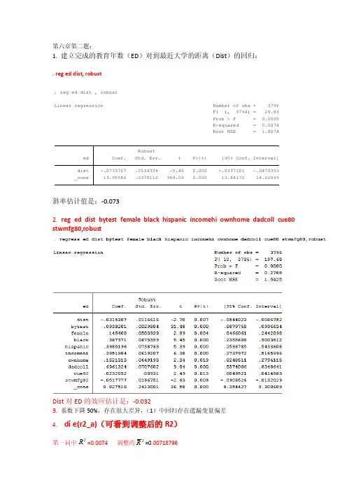
第六章第二题：1. 建立完成的教育年数（ED ）对到最近大学的距离（Dist ）的回归：. reg ed dist, robust斜率估计值是：-0.0732. reg ed dist bytest female black hispanic incomehi ownhome dadcoll cue80 stwmfg80,robustDist 对ED 的效应估计是：-0.0323. 系数下降50%，存在很大差异，（1）中回归存在遗漏变量偏差4. di e(r2_a)（可看到调整后的R2）第一问中=0.0074 调整的2R =0.00718796_cons 13.95586 .0378112 369.09 0.000 13.88172 14.02999dist -.0733727 .0134334 -5.46 0.000 -.0997101 -.0470353ed Coef. Std. Err. t P>|t| [95% Conf. Interval]RobustRoot MSE = 1.8074R-squared = 0.0074Prob > F = 0.0000F( 1, 3794) = 29.83Linear regression Number of obs = 3796. reg ed dist , robust2R第二问中=0.2788 2R = 0.27693235可以得到第二问中的拟合效果要优于第一问。

第二问中相似的原因：因为n 很大。

5. Dadcoll 父亲有没有念过大学：系数为正（0.6961324）衡量父亲念过大学的学生接受的教育年数平均比其父亲没有年过大学的学生多。

-.0517777 1）原因：这些参数在一定程度上构成了上大学的机会成本。

2）它们的系数估计值的符号应该如此。

当Stwmfg80增加时，放弃的工资增加，所以大学入学率降低了；因而Stwmfg80的系数对应为负。

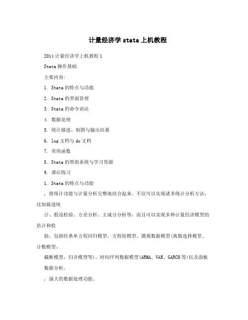
计量经济学stata上机教程2014计量经济学上机教程1Stata操作基础主要内容:1. Stata的特点与功能2. Stata的界面管理3. Stata的命令语法4. 数据处理5. 统计描述、制图与输出结果6. log文档与do文档7. 常用函数8. Stata的帮助系统与学习资源9. 课后练习1. Stata的特点与功能, 将统计功能与计量分析完整地结合起来。

不仅可以实现诸多统计分析方法，比如描述统计、假设检验、方差分析、主成分分析等，而且可以实现多种计量经济模型的估计和检验，包括经典单方程回归模型、方程组模型、微观数据模型(离散选择模型、计数模型、截断模型、归并模型等)、时间序列数据模型(ARMA、VAR、GARCH等)以及面板数据分析。

, 强大的数据处理功能。

, 精致的作图功能。

, 丰富的网络资源。

Stata 12有各种版本，其中尤以SE(特殊版)最为常用。

用户可以在命令栏中输入about命令查看所安装的版本信息。

2--per ml sodium hydroxide [c (NaOH) =1.000 mol/L] potassium hydrogen phthalate standard solution of quality g. ... After dilution to 1000mL. 1.1.2 0.000 35mol/L iodine solution: dissolve 20 g of potassium iodide in Cheng You (30~40) 500mL mL water bottle; 5mL iodine stock solution, and then diluted to scale and mix. This solution every other day to prepare. 1.1.3 acetate buffer (PH5.3): dissolve 87g sodium acetate (CH3COONa • 3H2O) 400mL water and 10.5mL in glacial acetic acid is dissolved in a small amount of water. volume and then mixing the two together and add water to 500mL, using regulation to PH5.3. 1.1.40.5mol/L sodium chloride: 14.5 g of sodium chloride dissolved in boiled water, and constant volume to 500mL. 1.1.5 soluble starch: pure before use should determine its value. Accurate said take amount starch (equivalent to dry state 1g) Yu 250mL high type beaker in the, added80~90mL distilled water, Yu asbestos online in constantly mixing Xia quickly heating to boiling, then with fire keep micro-boiling 3min, stamped and cooling to at room temperature, transfer to 100mL capacity bottle in the, into 40 ? water bath in the makes solution reached this temperature, and in 40 ? Shi with distilled water (40 ?) set capacity, this starch solution placed 40 ? thermostat water bath in the for determination samples with. 1.2 the instrument a) constant temperaturewater bath: (40+-0.2) 0C. B) spectrophotometer. 1.3 procedures 1.3.1 preparation of samples: weighing 50mL 10G sample不同的版本对于样本容量、变量个数、矩阵阶数等有着不同的限制，用户可以通过以下命令了解和改变这些设定:memory 显示目前存储空间query memory 查看目前实际设定的存储空间set memory 10m 设定存储空间的大小set matsize 250 设定最大矩阵阶数set maxvar 2500 设定最大变量数(最小设定为2048)help limits 显示Stata的各种极限 2. Stata的界面管理, 首次打开Stata，将会出现一个询问是否进行更新的对话框。

计量经济学stata操作（实验课）第一章stata基本知识1、stata窗口介绍2、基本操作（1）窗口锁定：Edit-preferences-general preferences-windowing-lock splitter （2）数据导入（3）打开文件：use E:\example.dta,clear（4）日期数据导入：gen newvar=date(varname, “ymd”)format newvar %td 年度数据gen newvar=monthly(varname, “ym”)format newvar %tm 月度数据gen newvar=quarterly(varname, “yq”)format newvar %tq 季度数据（5）变量标签Label variable tc ` “total output” ’（6）审视数据describelist x1 x2list x1 x2 in 1/5list x1 x2 if q>=1000drop if q>=1000keep if q>=1000（6）考察变量的统计特征summarize x1su x1 if q>=10000su q,detailsutabulate x1correlate x1 x2 x3 x4 x5 x6（7）画图histogram x1, width(1000) frequencykdensity x1scatter x1 x2twoway (scatter x1 x2) (lfit x1 x2)twoway (scatter x1 x2) (qfit x1 x2)（8）生成新变量gen lnx1=log(x1)gen q2=q^2gen lnx1lnx2=lnx1*lnx2gen larg=(x1>=10000)rename larg largeg large=(q>=6000)replace large=(q>=6000)drop ln*（8）计算功能display log(2)（9）线性回归分析regress y1 x1 x2 x3 x4vce #显示估计系数的协方差矩阵reg y1 x1 x2 x3 x4,noc #不要常数项reg y1 x1 x2 x3 x4 if q>=6000reg y1 x1 x2 x3 x4 if largereg y1 x1 x2 x3 x4 if large==0reg y1 x1 x2 x3 x4 if ～largepredict yhatpredict e1,residualdisplay 1/_b[x1]test x1=1 # F检验，变量x1的系数等于1test (x1=1) (x2+x3+x4=1) # F联合假设检验test x1 x2 #系数显著性的联合检验testnl _b[x1]= _b[x2]^2（10）约束回归constraint def 1 x1+x2+x3=1cnsreg y1 x1 x2 x3 x4,c(1)cons def 2 x4=1cnsreg y1 x1 x2 x3 x4,c(1-2)（11）stata的日志File-log-begin-输入文件名log off 暂时关闭log on 恢复使用log close 彻底退出（12）stata命令库更新Update allhelp command第二章有关大样本ols的stata命令及实例（1）ols估计的稳健标准差reg y x1 x2 x3,robust（2）实例use example.dta,clearreg y1 x1 x2 x3 x4test x1=1reg y1 x1 x2 x3 x4,rtestnl _b[x1]=_b[x2]^2第三章最大似然估计法的stata命令及实例（1）最大似然估计help ml（2）LR检验lrtest #对面板数据中的异方差进行检验（3）正态分布检验sysuse auto #调用系统数据集auto.dtahist mpg,normalkdensity mpg,normalqnorm mpg*手工计算JB统计量sum mpg,detaildi (r(N)/6)*((r(skewness)^2)+[(1/4)*(r(kurtosis)-3)^2])di chi2tail(自由度，上一步计算值)*下载非官方程序ssc install jb6jb6 mpg*正态分布的三个检验sktest mpgswilk mpgsfrancia mpg*取对数后再检验gen lnmpg=log(mpg)kdensity lnmpg, normaljb6 lnmpgsktest lnmpg第四章处理异方差的stata命令及实例（1）画残差图rvfplotrvfplot varname*例题use example.dta,clearreg y x1 x2 x3 x4rvfplot # 与拟合值的散点图rvfplot x1 # 画残差与解释变量的散点图（2）怀特检验estat imtest,white*下载非官方软件ssc install whitetst（3）BP检验estat hettest #默认设置为使用拟合值estat hettest,rhs #使用方程右边的解释变量estat hettest [varlist] #指定使用某些解释变量estat hettest,iidestat hettest,rhs iidestat hettest [varlist],iid（4）WLSreg y x1 x2 x3 x4 [aw=1/var]*例题quietly reg y x1 x2 x3 x4predict e1,resgen e2=e1^2gen lne2=log(e2)reg lne2 x2,nocpredict lne2fgen e2f=exp(lne2f)reg y x1 x2 x3 x4 [aw=1/e2f]（5）stata命令的批处理（写程序）Window-do-file editor-new do-file#WLS for examplelog using E:\wls_example.smcl,replaceset more offuse E:\example.dta,clearreg y x1 x2 x3 x4predict e1,resgen e2=e1^2g lne2=log(e2)reg lne2 x2,nocpredict lne2fg e2f=exp(lne2f)*wls regressionreg y x1 x2 x3 x4 [aw=1/e2f]log closeexit第五章处理自相关的stata命令及实例（1）滞后算子/差分算子tsset yearl.l2.D.D2.LD.（2）画残差图scatter e1 l.e1ac e1pac e1（3）BG检验estat bgodfrey（默认p=1）estat bgodfrey,lags(p)estat bgodfrey,nomiss0（使用不添加0的BG检验）（4）Ljung-Box Q检验reg y x1 x2 x3 x4predict e1,residwntestq e1wntestq e1,lags(p)* wntestq指的是“white noise test Q”，因为白噪声没有自相关（5）DW检验做完OLS回归后，使用estat dwatson（6）HAC稳健标准差newey y x1 x2 x3 x4,lag(p)reg y x1 x2 x3 x4,cluster(varname)（7）处理一阶自相关的FGLSprais y x1 x2 x3 x4 （使用默认的PW估计方法）prais y x1 x2 x3 x4,corc （使用CO估计法）（8）实例use icecream.dta, cleartsset timegraph twoway connect consumption temp100 time, msymbol(circle) msymbol(triangle) reg consumption temp price incomepredict e1, resg e2=l.e1twoway (scatter e1 e2) (lfit e1 e2)ac e1pac e1estat bgodfreywntestq e1estat dwatsonnewey consumption temp price income, lag (3)prais consumption temp price income, corcprais consumption temp price income, nologreg consumption temp l.temp price incomeestat bgodfreyestat dwatson第六章模型设定与数据问题（1）解释变量的选择reg y x1 x2 x3estat ic*例题use icecream.dta, clearreg consumption temp price incomeestat icreg consumption temp l.temp price incomeestat ic（2）对函数形式的检验（reset检验）reg y x1 x2 x3estat ovtest （使用被解释变量的2、3、4次方作为非线性项）estat ovtest, rhs （使用解释变量的幂作为非线性项，ovtest-omitted variable test）*例题use nerlove.dta, clearreg lntc lnq lnpl lnpk lnpfestat ovtestg lnq2=lnq^2reg lntc lnq lnq2 lnpl lnpk lnpfestat ovtest（3）多重共线性estat vif*例题use nerlove.dta, clearreg lntc lnq lnpl lnpk lnpfestat vif（4）极端数据reg y x1 x2 x3predict lev, leverage （列出所有解释变量的lev值）gsort –levsum levlist lev in 1/3*例题use nerlove.dta, clearquietly reg lntc lnq lnpl lnpk lnpfpredict lev, leveragesum levgsort –levlist lev in 1/3（5）虚拟变量gen d=(year>=1978)tabulate province, generate (pr)reg y x1 x2 x3 pr2-pr30（6）经济结构变动的检验方法1：use consumption_china.dta, cleargraph twoway connect c y year, msymbol(circle) msymbol(triangle)reg c yreg c y if year<1992reg c y if year>=1992计算F统计量方法2：gen d=(year>1991)gen yd=y*dreg c y d ydtest d yd第七章工具变量法的stata命令及实例（1）2SLS的stata命令ivregress 2sls depvar [varlist1] (varlist2=instlist)如：ivregress 2sls y x1 (x2=z1 z2)ivregress 2sls y x1 (x2 x3=z1 z2 z3 z4) ,r firstestat firststage,all forcenonrobust （检验弱工具变量的命令）ivregress liml depvar [varlist 1] (varlist2=instlist)estat overid （过度识别检验的命令）*对解释变量内生性的检验（hausman test），缺点：不适合于异方差的情形reg y x1 x2estimates store olsivregress 2sls y x1 (x2=z1 z2)estimates store ivhausman iv ols, constant sigmamore*DWH检验estat endogenous*GMM的过度识别检验ivregress gmm y x1 (x2=z1 z2) （两步GMM）ivregress gmm y x1 (x2=z1 z2),igmm （迭代GMM）estat overid*使用异方差自相关稳健的标准差GMM命令ivregress gmm y x1 (x2=z1 z2), vce (hac nwest[#])（2）实例use grilic.dta,clearsumcorr iq sreg lw s expr tenure rns smsa,rreg lw s iq expr tenure rns smsa,rivregress 2sls lw s expr tenure rns smsa (iq=med kww mrt age),restat overidivregress 2sls lw s expr tenure rns smsa (iq=med kww),r firstestat overidestat firststage, all forcenonrobust （检验工具变量与内生变量的相关性）ivregress liml lw s expr tenure rns smsa (iq=med kww),r*内生解释变量检验quietly reg lw s iq expr tenure rns smsaestimates store olsquietly ivregress 2sls lw s expr tenure rns smsa (iq=med kww)estimates store ivhausman iv ols, constant sigmamoreestat endogenous （存在异方差的情形）*存在异方差情形下，GMM比2sls更有效率ivregress gmm lw s expr tenure rns smsa (iq=med kww)estat overidivregress gmm lw s expr tenure rns smsa (iq=med kww),igmm*将各种估计方法的结果存储在一张表中quietly ivregress gmm lw s expr tenure rns smsa (iq=med kww)estimates store gmmquietly ivregress gmm lw s expr tenure rns smsa (iq=med kww),igmmestimates store igmmestimates table gmm igmm第八章短面板的stata命令及实例（1）面板数据的设定xtset panelvar timevarencode country,gen(cntry) （将字符型变量转化为数字型变量）xtdesxtsumxttab varnamextline varname,overlay*实例use traffic.dta,clearxtset state yearxtdesxtsum fatal beertax unrate state yearxtline fatal（2）混合回归reg y x1 x2 x3,vce(cluster id)如：reg fatal beertax unrate perinck,vce(cluster state)estimates store ols对比：reg fatal beertax unrate perinck（3）固定效应xtreg y x1 x2 x3,fe vce(cluster id)xi:reg y x1 x2 x3 i.id,vce(cluster id) （LSDV法）xtserial y x1 x2 x3,output （一阶差分法，同时报告面板一阶自相关）estimates store FD*双向固定效应模型tab year, gen (year)xtreg fatal beertax unrate perinck year2-year7, fe vce (cluster state)estimates store FE_TWtest year2 year3 year4 year5 year6 year7（4）随机效应xtreg y x1 x2 x3,re vce(cluster id) （随机效应FGLS）xtreg y x1 x2 x3,mle （随机效应MLE）xttest0 （在执行命令xtreg, re 后执行，进行LM检验）（5）组间估计量xtreg y x1 x2 x3,be（6）固定效应还是随机效应：hausman testxtreg y x1 x2 x3,feestimates store fextreg y x1 x2 x3,reestimates store rehausman fe re,constant sigmamore （若使用了vce(cluster id)，则无法直接使用该命令，解决办法详见P163）estimates table ols fe_robust fe_tw re be, b se （将主要回归结果列表比较）第九章长面板与动态面板（1）仅解决组内自相关的FGLSxtpcse y x1 x2 x3 ,corr(ar1) （具有共同的自相关系数）xtpcse y x1 x2 x3 ,corr(psar1) （允许每个面板个体有自身的相关系数）例题：use mus08cigar.dta,cleartab state,gen(state)gen t=year-62reg lnc lnp lnpmin lny state2-state10 t,vce(cluster state)estimates store OLSxtpcse lnc lnp lnpmin lny state2-state10 t,corr(ar1) (考虑存在组内自相关，且各组回归系数相同)estimates store AR1xtpcse lnc lnp lnpmin lny state2-state10 t,corr(psar1) (考虑存在组内自相关，且各组回归系数不相同)estimates store PSAR1xtpcse lnc lnp lnpmin lny state2-state10 t, hetonly (仅考虑不同个体扰动性存在异方差，忽略自相关)estimates store HETONL Yestimates table OLS AR1 PSAR1 HETONL Y, b se（2）同时处理组内自相关与组间同期相关的FGLSxtgls y x1 x2 x3,panels (option/iid/het/cor) corr(option/ar1/psar1) igls注：执行上述xtpcse、xtgls命令时，如果没有个体虚拟变量，则为随机效应模型；如果加上个体虚拟变量，则为固定效应模型。

计量经济学上机命令整理实验一edit 打开数据编辑器browse 打开数据浏览器rename 对变量重新命名labelsavedescribe 对数据集简要描述sort 排序例如:list in -10/-1list 显示变量的数值Generate 缩小:gen 生成新的变量后面可以接if条件句Replace 替换append 覆盖Summarize 缩写:su 总结后面可以接if条件句实验二twoway (scatter y x)(connected ey_x x) 在该散点图上,做出条件均值点sc y x||lfit y x 画出线图和散点图Reg y x 做出回归Rename ** y **指原变量名用于修改变量名字graph twoway scatter y x 画出y x 的二维散点图Line y x 做出y x 的线条图egen Ey_x=mean(y),by(x) 求在同一x水平下,求y的均值实验三Regress y x1 x2 ........做多元回归Precict e,re 预测方差Sort e 按照方差排序Cor y x 测试y与x的相关程度Pwcorr y x 也是测试y与x的相关程度Set obs 90 (90为任意一个数字),增加一个或者多个样本值Replace x=980 in 90 为第90个样本值赋值(980为任意一个数字)Predict yhat 预测y的估计值Display invttail(n,p) n为自由度;p为概率(一般为0.025)。

用来求t分布的t 值Display ttail(n,t)知道t值求T<t的右端概率Destring (变量名,可省略),replace ignore("-$") 将其他类型的数据转化为数值型Hist e残差直方图hist e,norm加了一条正态分布线Two connected y x 二维图连线Two connected y x,yline(0) 在y=0处画一条线(也可x=0)Kdensity e,normal 对残差画出密度图Sktest e 利用e的偏锋度做是否符合正态分布的检验gen low=yhat-t*se gen high=yhat+t*se 预测置信区间Twoway lfitci y x 置信区间与回归之间作图实验四(第五章)Gen lny=log(y)生成y的对数Gen lnx=log(x)生成x的对数Drop y或者x 删除变量Predict se,stdp 预测所有的标准误实验五(第六章)虚拟变量Tab quarter,gen(d) quarter代表变量,对变量quarter生成虚拟变量d Gen d1_x=d1*x 或者是(d2,d3,d4与x2,x3,x4)生成交互作用的虚拟变量Reg y x1 x2...d2 d3 d4.....(d1通常省略,常数项)Egen ybar=mean(y) 生成y的均值实验六(第八章:多重共线性)Gen t=0Replace t=1 if x<(或>或>=或<=)数值Test (t=0)(t_x=0)做假设联合检验,求出新的F值Test (lnx2+lnx3=1) 求出新的F检验统计量Cor lnx2-lnx6 求lnx2与lnx3到Lnx6之间的相关程度,找出是否存在多重共线性问题Pcorr lnx2 lnx3-lnx6 也是测量变量之间的相关程度Estat vif 估计方差膨胀因子(方差膨胀因子越大,说明两个此变量与y的共线性越高,应该考虑删除)实验七八(第九十章)Predict e,reGen e2=e^2Est store m1 记录原回归的内容Est tab m1 m2 展示上述记录过的回归内容并作出比较Est tab m1 m2.....,seEstat imtest 怀特检验Estat hettest BP检验Regress y x2 x3...,robust 校正后的怀特检验自相关检验Regress y x...Est store m1Predict e,reSc e obs,yline(0)Tsset obs或者其他变量,用来表示时间变化Dwstat 进行DW检验并查表得出自相关程度Gen rho=1-d/2 rho 代表ρ估计Prais y x,corc (one,two...)括号可接可不接表示从OLS残差中估计ρ Gen dy1=y-l.y*ρ1Gen dx1=y-l.y*ρ1Gen dy2=y-l.y*ρ2Gen dx2=y-l.y*ρ2 (rho=ρ)Replace dy1=sqrt(1-rho^2)*y if ......补充第一个样本值比如ifobs==1958 Replace dx1=sqrt(1-rho^2)*x if .......。

计量经济学stata上机教程2014计量经济学上机教程1Stata操作基础主要内容:1. Stata的特点与功能2. Stata的界面管理3. Stata的命令语法4. 数据处理5. 统计描述、制图与输出结果6. log文档与do文档7. 常用函数8. Stata的帮助系统与学习资源9. 课后练习1. Stata的特点与功能, 将统计功能与计量分析完整地结合起来。

不仅可以实现诸多统计分析方法，比如描述统计、假设检验、方差分析、主成分分析等，而且可以实现多种计量经济模型的估计和检验，包括经典单方程回归模型、方程组模型、微观数据模型(离散选择模型、计数模型、截断模型、归并模型等)、时间序列数据模型(ARMA、VAR、GARCH等)以及面板数据分析。

, 强大的数据处理功能。

, 精致的作图功能。

, 丰富的网络资源。

Stata 12有各种版本，其中尤以SE(特殊版)最为常用。

用户可以在命令栏中输入about命令查看所安装的版本信息。

2--per ml sodium hydroxide [c (NaOH) =1.000 mol/L] potassium hydrogen phthalate standard solution of quality g. ... After dilution to 1000mL. 1.1.2 0.000 35mol/L iodine solution: dissolve 20 g of potassium iodide in Cheng You (30~40) 500mL mL water bottle; 5mL iodine stock solution, and then diluted to scale and mix. This solution every other day to prepare. 1.1.3 acetate buffer (PH5.3): dissolve 87g sodium acetate (CH3COONa • 3H2O) 400mL water and 10.5mL in glacial acetic acid is dissolved in a small amount of water. volume and then mixing the two together and add water to 500mL, using regulation to PH5.3. 1.1.40.5mol/L sodium chloride: 14.5 g of sodium chloride dissolved in boiled water, and constant volume to 500mL. 1.1.5 soluble starch: pure before use should determine its value. Accurate said take amount starch (equivalent to dry state 1g) Yu 250mL high type beaker in the, added80~90mL distilled water, Yu asbestos online in constantly mixing Xia quickly heating to boiling, then with fire keep micro-boiling 3min, stamped and cooling to at room temperature, transfer to 100mL capacity bottle in the, into 40 ? water bath in the makes solution reached this temperature, and in 40 ? Shi with distilled water (40 ?) set capacity, this starch solution placed 40 ? thermostat water bath in the for determination samples with. 1.2 the instrument a) constant temperaturewater bath: (40+-0.2) 0C. B) spectrophotometer. 1.3 procedures 1.3.1 preparation of samples: weighing 50mL 10G sample不同的版本对于样本容量、变量个数、矩阵阶数等有着不同的限制，用户可以通过以下命令了解和改变这些设定:memory 显示目前存储空间query memory 查看目前实际设定的存储空间set memory 10m 设定存储空间的大小set matsize 250 设定最大矩阵阶数set maxvar 2500 设定最大变量数(最小设定为2048)help limits 显示Stata的各种极限 2. Stata的界面管理, 首次打开Stata，将会出现一个询问是否进行更新的对话框。

计量经济学stata上机教程计量经济学stata上机教程2014计量经济学上机教程1Stata操作基础主要内容:1. Stata的特点与功能2. Stata的界面管理3. Stata的命令语法4. 数据处理5. 统计描述、制图与输出结果6. log文档与do文档7. 常用函数8. Stata的帮助系统与学习资源9. 课后练习1. Stata的特点与功能, 将统计功能与计量分析完整地结合起来。

不仅可以实现诸多统计分析方法，比如描述统计、假设检验、方差分析、主成分分析等，而且可以实现多种计量经济模型的估计和检验，包括经典单方程回归模型、方程组模型、微观数据模型(离散选择模型、计数模型、截断模型、归并模型等)、时间序列数据模型(ARMA、VAR、GARCH等)以及面板数据分析。

, 强大的数据处理功能。

, 精致的作图功能。

, 丰富的网络资源。

Stata 12有各种版本，其中尤以SE(特殊版)最为常用。

用户可以在命令栏中输入about命令查看所安装的版本信息。

2--per ml sodium hydroxide [c (NaOH) =1.000 mol/L] potassium hydrogen phthalate standard solution of quality g. ... After dilution to 1000mL. 1.1.2 0.000 35mol/L iodine solution: dissolve 20 g of potassium iodide in Cheng You (30~40) 500mL mL water bottle; 5mL iodine stock solution, and then diluted to scale and mix. This solution every other day to prepare. 1.1.3 acetate buffer (PH5.3): dissolve 87g sodium acetate (CH3COONa ? 3H2O) 400mL water and 10.5mL in glacial acetic acid is dissolved in a small amount of water. volume and then mixing the two together and add water to 500mL, using regulation to PH5.3.1.1.40.5mol/L sodium chloride: 14.5 g of sodium chloride dissolved in boiled water, and constant volume to 500mL. 1.1.5 soluble starch: pure before use should determine its value. Accurate said take amount starch (equivalent to dry state 1g) Yu 250mL high type beaker in the, added80~90mL distilled water, Yu asbestos online in constantly mixing Xia quickly heating to boiling, then with fire keep micro-boiling 3min, stamped and cooling to at room temperature, transfer to 100mL capacity bottle in the, into 40 ? water bath in the makes solution reached this temperature, and in 40 ? Shi with distilled water (40 ?) set capacity, this starch solution placed 40 ? thermostat water bath in the for determination samples with. 1.2 the instrument a) constant temperaturewater bath: (40+-0.2) 0C. B) spectrophotometer. 1.3 procedures 1.3.1 preparation of samples: weighing 50mL 10G sample不同的版本对于样本容量、变量个数、矩阵阶数等有着不同的限制，用户可以通过以下命令了解和改变这些设定:memory 显示目前存储空间query memory 查看目前实际设定的存储空间set memory 10m 设定存储空间的大小set matsize 250 设定最大矩阵阶数set maxvar 2500 设定最大变量数(最小设定为2048)help limits 显示Stata的各种极限 2. Stata的界面管理, 首次打开Stata，将会出现一个询问是否进行更新的对话框。