东北大学DIP实验一

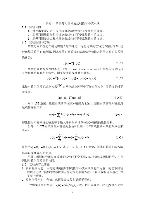
实验一 离散时间信号通过线性时不变系统1.1 实验目的1、通过本实验，进一步加深对离散线性时不变系统的理解。

2、掌握利用线性卷积求解离散线性时不变系统输出的方法。

3、掌握利用差分方程求解离散线性时不变系统输出的方法。

1.2 实验原理与方法离散时间系统的作用是将输入序列通过一定的运算处理转变为输出序列,这种运算关系用[]T ∙表示，因此离散时间系统的输出信号和输入信号之间的关系可描述为：()[()]y n T x n = （1-1）离散时间系统线性时不变（LTI Linear time-invariant ）的特点是系统具有线性性质和时不变特性。

即系统满足线性叠加原理。

1212()[()()]()()y n T ax n bx n ay n by n =+=+ （1-2） 系统对输入信号的运算关系[]T ∙在整个运算过程中不随时间变化，即系统是时不变系统：()[()]y n i T x n i -=- （1-3）对于LTI 系统，设该系统的单位脉冲响应为h(n)，则该系统的输入输出满足线性卷积关系：()()()()()i y n h i x n i x n h n +∞=-∞=-=*∑ （1-4） 即线性时不变系统的输出等于输入序列与系统单位脉冲响应的线性卷积。

另外一个LTI 系统的输入输出关系还可以用一个N 阶线性常系数差分方程来表示：0()()()M Ni i i i i y n b x n i a y n i ===---∑∑ （1-5）显然当0,0,1,2,,i a i N == 时，式（1-4）与（1-5）等价，即此时系统的输入输出满足线性卷积的关系。

另外：周期信号通过离散时间线性时不变系统，输出仍然是周期信号，并且周期与输入信号周期相同。

1.3 实验内容及步骤1. 在实验编程前，认真复习离散时间线性时不变系统的有关内容，阅读本实验原理与方法，掌握线性卷积和差分方程的求解方法，了解单载波信号通过LTI 系统的特性。

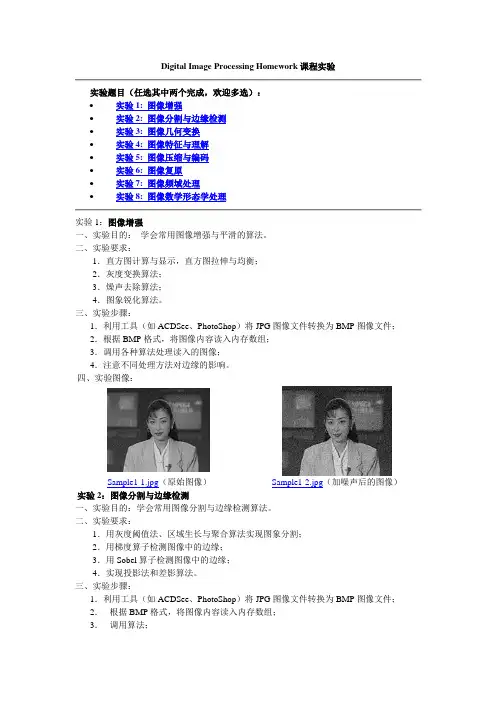
Digital Image Processing Homework课程实验实验题目（任选其中两个完成，欢迎多选）：∙实验1: 图像增强∙实验2: 图像分割与边缘检测∙实验3: 图像几何变换∙实验4: 图像特征与理解∙实验5: 图像压缩与编码∙实验6: 图像复原∙实验7: 图像频域处理∙实验8: 图像数学形态学处理实验1：图像增强一、实验目的：学会常用图像增强与平滑的算法。

二、实验要求：1．直方图计算与显示，直方图拉伸与均衡；2．灰度变换算法；3．燥声去除算法；4．图象锐化算法。

三、实验步骤：1．利用工具（如ACDSee、PhotoShop）将JPG图像文件转换为BMP图像文件；2．根据BMP格式，将图像内容读入内存数组；3．调用各种算法处理读入的图像；4．注意不同处理方法对边缘的影响。

四、实验图像：Sample1-1.jpg（原始图像）Sample1-2.jpg（加噪声后的图像）实验2：图像分割与边缘检测一、实验目的：学会常用图像分割与边缘检测算法。

二、实验要求：1．用灰度阈值法、区域生长与聚合算法实现图象分割；2．用梯度算子检测图像中的边缘；3．用Sobel算子检测图像中的边缘；4．实现投影法和差影算法。

三、实验步骤：1．利用工具（如ACDSee、PhotoShop）将JPG图像文件转换为BMP图像文件；2．根据BMP格式，将图像内容读入内存数组；3．调用算法；4．比较处理结果。

四、实验图像：Sample2-1.jpg Sample2-2.jpg实验3：图像几何变换1、Image Printing Program Based on Halftoning (Pattern 半影调法，图案法)The following figure shows ten shades of gray approximated by dot patterns. Each gray level is represented by a 3 x 3 pattern of black and white dots. A 3 x 3 area full of black dots is the approximation to gray-level black, or 0. Similarly, a 3 x 3 area of white dotsrepresents gray level 9, or white. The other dot patterns are approximations to gray levels in between these two extremes. A gray-level printing scheme based on dots patterns such as these is called "halftoning" Note that each pixel in an input image will correspond to 3 x 3 pixels on the printed image, so spatial resolution will be reduced to 33% of the original in both the vertical and horizontal direction. Size scaling as required in (a) may furtherreduce resolution, depending on the size of the input image.(a) Write a halftoning computer program for printing gray-scale images based on the dotpatterns just discussed. Your program must be able to scale the size of an input image so that it does not exceed the area available in a sheet of size A4 (21.6 x 27.9 cm). Yourprogram must also scale the gray levels of the input image to span the full halftoning range.(b) Write a program to generate a test pattern image consisting of a gray scale wedge ofsize 256 x 256, whose first column is all 0's, the next column is all 1's, and so on, with the last column being 255's. Print this image using your gray-scale printing program.(c) Print iamges Sample4-1.jpg, Sample4-2.jpg and Sample4-3.jpg using your gray-scaleprinting program.2、Reducing the Number of Gray Levels in an Image （二值化）(a) Write a computer program capable of reducing the number of gray levels in a image from 256 to 2, in integer powers of 2. The desired number of gray levels needs to be a variable input to your program.(b) Download the image Sample4-4.jpg and run your program.3、Zooming and Shrinking Images by Pixel Replication （基于像素插补的放大缩小） (a) Write a computer program capable of zooming and shrinking an image by pixelreplication （插补）. Assume that the desired zoom/shrink factors are integers. You may ignore aliasing effects.(b) Download the image Sample4-5.jpg and use your program to shrink the image from 1024 x 1024 to 256 x 256 pixels.(c) Use your program to zoom the image in (b) back to 1024 x 1024. Explain the reasons for their differences.4、Zooming and Shrinking Images by Bilinear Interpolation （基于双线性插值的放大缩小）(a) Write a computer program capable of zooming and shrinking an image by bilinear interpolation. The input to your program is the desired size of the resulting image in the horizontal and vertical direction. You may ignore aliasing effects.(b) Download the image Sample4-5.jpg and use your program to shrink this image from 1024 x 1024 to 256 x 256 pixels.(c) Use your program to zoom the image in (b) back to 1024 x 1024. Explain the reasonsfor their differencesSample4-1.jpgSample4-2.jpgSample4-3.jpgSample4-4.jpgSample4-5.jpg实验4：图像特征与理解实验5：图像压缩与编码一、实验目的：掌握数字图像的基本压缩与编码技术。

第二章 89C51单片机的结构和原理A TMEL 、PHLIPS 和SST 等公司生产的8位单片机89C51与80C51兼容，具有低功耗高性能的特点，特别是在内部增加了闪速存储器Flash ROM ，给单片机系统的开发应用带来很大方便，近年来得到非常广泛的应用。

本章以A T89C51为基础，详细介绍芯片的内部硬件资源、各功能部件的结构和原理。

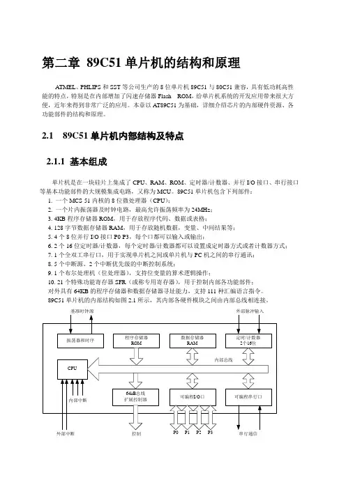
2.1 89C51单片机内部结构及特点 2.1.1 基本组成单片机是在一块硅片上集成了CPU 、RAM 、ROM 、定时器/计数器、并行I/O 接口、串行接口 等基本功能部件的大规模集成电路，又称为MCU 。

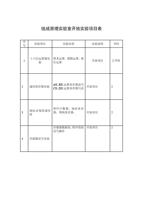
89C51单片机包含下列部件： 1. 一个MCS-51内核的8位微处理器（CPU ）； 2. 一个片内振荡器及时钟电路，最高允许振荡频率为24MHz ； 3. 4KB 程序存储器ROM ，用于存放程序代码、数据或表格；4. 128字节数据存储器RAM ，用于存放随机数据，变量、中间结果等；5. 4个8位并行I/O 接口P0-P3，每个口都可以输入或输出；6. 2个16位定时器/计数器，每个定时器/计数器都可以设置成定时器方式或者计数器方式；7. 1个全双工串行口，用于实现单片机之间或单片机与PC 机之间的串行通讯；8. 5个中断源、2个中断优先级的中断控制系统；9. 1个布尔处理机（位处理器），支持位变量的算术逻辑操作； 10. 21个特殊功能寄存器SFR （或称专用寄存器），用于控制内部各功能部件； 对外具有64KB 的程序存储器和数据存储器寻址能力，支持111种汇编语言指令。

89C51单片机的内部结构如图2.1所示，其内部各硬件模块之间由内部总线相连接。

外部中断控制串行通信外部脉冲输入基准时钟源图2.1 MCS-89C51单片机的结构框图上图中，存储器容量和定时器/计数器数量随子型号的不同而有变化，见表2.1。

89C51是一种低功耗、低电压、高性能的8位单片机。

ESP工艺下DP600热轧双相钢铁素体相变模型
周晓光;马鑫;姜珊;刘振宇
【期刊名称】《东北大学学报（自然科学版）》
【年(卷),期】2024(45)4
【摘要】为了建立ESP工艺条件下DP600热轧双相钢的铁素体相变动力学数学模型,采用动态相变膨胀仪对实验钢分别进行等温相变和连续冷却相变实验.基于实测的铁素体相变孕育期和铁素体体积分数,在变形温度以上结合经典形核理论计算铁素体相变孕育期,变形温度以下通过实验数据拟合△GV计算铁素体相变孕育期.考虑冷却速度的影响对可加性法则进行修正并基于此计算了连续冷却条件下的铁素体相变开始温度和体积分数.结果表明:修正后的相变模型计算的铁素体相变开始温度和体积分数与实测值吻合良好,可用于预测ESP工艺下DP600钢的铁素体相变行为.
【总页数】7页(P483-489)
【作者】周晓光;马鑫;姜珊;刘振宇
【作者单位】东北大学轧制技术及连轧自动化国家重点实验室
【正文语种】中文
【中图分类】TG142
【相关文献】
1.超快冷条件下含Nb钢铁素体相变区析出及模型研究
2.工艺参数对600MPa热轧双相钢铁素体转变的影响
3.变形、冷却条件下低碳钢铁素体相变的元胞自动机模型
4.基于FTSR热轧含Nb钢的铁素体相变实际转变温度模型
因版权原因，仅展示原文概要，查看原文内容请购买。