R. Automatic camera calibration and scene reconstruction with scale-invariant features

双目立体相机自标定方案的研究一、双目立体相机自标定原理双目视觉是通过两个摄像机从不同的角度拍摄同一物体，根据两幅图像重构出物体。

双目立体视觉技术首先根据已知信息计算出世界坐标系和图像坐标系的转换关系，即世界坐标系和图像坐标系的透视投影矩阵，将两幅图像上对应空间同一点的像点匹配起来，建立对应点的世界坐标和图像坐标的转换关系方程，通过求解方程的最小二乘解获取空间点的世界坐标系，实现二维图像到三维图像的重构。

重构的关键问题是找出世界坐标系和图像坐标系的转换关系--透视投影矩阵。

透视投影矩阵包含了图像坐标系和相机坐标系的转换关系，即相机的内参（主要是相机在两坐标轴上的焦距和相机的倾斜角度），以及相机坐标系和世界坐标系的转换关系，即相机的外参（主要是相机坐标系和世界坐标系的平移、旋转量）。

相机标定的过程就是确定相机内参和相机外参的过程。

相机自标定是指不需要标定块，仅仅通过图象点之间的对应关系对相机进行标定的过程。

相机自标定技术不需要计算出相机的每一项参数，但需要求出这些参数联系后生成的矩阵。

二、怎样提高摄像机自标定精确度？方法一、.提高估算基本矩阵F传统的相机自标定采用的是kruppa方程，一组图像可以得到两个kruppa方程，在已知3对图像的条件下，就可以算出所有的内参数。

在实际应用中，由于求极点具有不稳定性，所以采取基本矩阵F分解的方法来计算。

通过矩阵的分解求出两相机的投射投影矩阵，进而实现三维重构。

由于在获取图像过程中存在摄像头的畸变，环境干扰等因素，对图像会造成非线性变化，采用最初提出的线性模型计算 f 会产生误差。

非线性的基本矩阵估计方法得到提出。

近年来非线性矩阵的新发展是通过概率模型降低噪声以提高估算基本矩阵的精度。

方法二、分层逐步标定法。

该方法首先对图像做射影重建，再通过绝对二次曲线施加约束，定出仿射参数和摄像机参数。

由于它较其他方法具有较好的鲁棒性，所以能提高自标定的精度。

方法三、利用多幅图像之间的直线对应关系的标定法。

UBC机器人照相机校准操作方法
激活这个功能按钮
在画面里选择你要校准的照相机
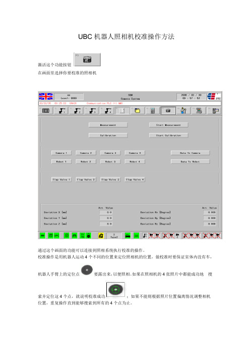
通过这个画面的功能可以连接到照相系统执行校准的操作。

校准操作是用机器人运动4个不同的位置来定位照相机的位置，做校准时要保证室体内没有车，
机器人手臂上的定位点要露出来，以便照相。

如果在照相机的4张照片中都能成功地搜
索并定位这4个点，就说明校准成功；如果不能则根据照片位置偏离情况调整相机位置，重复操作直到能够搜索到所有的4个点为止。

操作控制按钮如下：（不限于校准）。

An Implementation of Camera Calibration AlgorithmsMeredith DrennanDepartment of Electrical and Computer EngineeringClemson UniversityAbstractCamera calibration is an important preprocessing step in computer vision applications. This paper seeks to provide an introduction to camera calibration procedures. It also discusses an implementation of automating point correspondences in known planar objects. Finally, results of a new implementation of Zhang’s calibration procedure are compared to other open source implementation results.1.IntroductionComputer vision is inherently plagued by the loss of dimensionality incurred when capturing a 3D photo in a 2D image. Camera calibration is an important step towards recovering three-dimensional information from a planar image. Over the past twenty years several algorithms have proposed solutions to the problem of calibration. Among the most popular are Roger Tsai’s algorithm [5], Direct Linear Transformation (DLT), and Zhang’s algorithm[6]. The focus of this paper is on Zhang’s algorithm because it is the basis behind popular open source implementations of camera calibration i.e. Intel’s Open CV and Matlab’s calibration toolkit [1].2.MethodsCalibration relates known points in the world to points in an image, in order to do so one must first acquire a series of known world points. The most common method is to use known planar objects at different orientations with respect to the camera to develop an independent series of data points. The calibration object chosen in this implementation is a 6x6 checkerboard with the corner points as the known world points. Most corner detector algorithms for camera calibration use edge detection to find the structure of the checkerboard, fit lines to the data points and compute the intersection of the lines in order to find the corners. This technique can be very accurate, providing in some cases accuracy of better than one tenth of a pixel but requires complicated line fitting algorithms. The implementation used here is based on feature detection by pinpointing windows with high variances in the X and Y directions. The points corresponding to the 36 highest variances (6x6 checkerboard implies 36 corners) are then chosen as the corner points. A simple image masking technique is used to ensure that no corner is detected twice. This is a much simpler implementation but experimental results show that accuracy is lost (see results section).The corners may be transformed into world points by assuming an origin at the top left corner of the checkerboard and then imposing the constant distance of each square between neighboring corners.Once a series of world points have been developed the homography matrix must be computed. This matrix becomes essentially a3x3 matrix relating world points to image points. The homography (H) can then be processed into intrinsic parameter (A), rotation, and translation matrices. We may assume that Z = 0 without loss of generality because a planar object is used to perform the calibration [6].The steps to compute the homography and intrinsic parameter matrices are as follows:sm = H M(1)Where m = [u, v, 1]T in the image plane coordinates and M = [x, y, 1]T in the model plane coordinates. From equation 1, the homography may be determined to within a scale factor (s).Computing the homography matrix takes the following form (from [2]): [x 1, y 1, 1, 0, 0, 0, -u 1x 1, -u 1y 1, -u 1,0, 0, 0, x 1, y 1, 1, -v 1x 1, -v 1y 1, -v1(2)x n , y n , 1, 0, 0, 0, -u n x n , -u n y n , -u n ,0, 0, 0, x n , y n , 1, -v n x n , -v n y n , -v n ]h’ = 0 Where h’ is a 9x1 column vector to be reshaped into the 3x3 homography H . By stacking this equation for n points in an image, the over-determined system can be solved using the eigen vector associated with the second smallest eigen value found via the SVD.Note that equation 2 introduced a matrix whose elements have various units, some of pixels, some meters, and some pixels*meters. It is important to normalize this matrix in order to achieve more stable results in the output.The following normalization matrix is used [4](3)where w and h are the image width and height respectively.Once H has been calculated the value of matrix B is estimatedB =(4)B is a symmetric 3x3 matrixLet b = [B11 B12 B22 B13 B23 B33] (5) andVij = [h i h ji , h i1h j2+h i2h j1, h i2h j2, h i3h j1+h i1h j3,h i3h j2+h i2h j3, h i3h j3](6)G =(15)The intrinsic matrix, A can then be found by denormalizing A’A = N-1A’ (16)For more information on the preceding algorithms see [3], [4], [6]. Further calculations can be done to find the rotation and translation matrices corresponding to each image and the first and second order distortion coefficients as described in [6].3.ResultsCode has been written in C++ in order to test the accuracy of the algorithms for feature detection and Zhang’s method discussed previously. As a baseline, the same camera (Dynex DX-WEB1C webcam) was also calibrated using two common open source implementations of Zhang’s calibration; Matlab’s toolkit available on the web [2], and Intel’s Open CV implementation. The number of input images to all three calibration tools has been kept constant at three. Using Blepo’s demo implementation of the Open CV code requires a nine square by six checkerboard input while both Matlab and the author’s version received the same 6x6 checkerboard images, therefore roughly the same data was fed to all three versions.A.Corner DetectionUsing a standard feature detection algorithm which searches for areas of high variances in X and Y directions, accuracy can be obtained at an average of within 2.2 pixels with a standard deviation of 1.4. While this is clearly not as accurate as calibration tools which use line fitting techniques, the prime advantage of this method of corner detection is simplicity.Figure 1 Checkerboard Variances and CornersFigure 1 shows an output of the feature detection on a standard checkerboard. Lines in gray mark areas of high variance in the X direction, and lines in white indicate areas of high variance in the Y direction. The points in blue mark the possible corners.A standard sort algorithm finds the areas of highest variance. Two techniques are used to ensure that a corner is not detected twice, first the image is fed to a Canny edge detector in order to reduce the number of possible corners. Then an image mask ensures that no other pointwithin 15 pixels is marked as a corner.Figure 2 Corners FoundB.Calibration AlgorithmOnce the corners have been detected, the calibration algorithm performs a series of steps as indicated in the methods section. The outputof the calibration is an intrinsic parameter matrix (A ) whose elements are described below andcompared to Matlab and Open CV results.Figure 1 Principle PointFigure 1 shows the observed principle point according to each implementation. All shown estimations are reasonable as the expected principle point would be at the center. Forreference purposes a pink square is drawn at the center of the image.The matrix A also contains values of α and β, where α/ β is the ratio of pixel width to height and is equal to 1 for most standard cameras. For the given camera this ratio averages at .9998 in Open CV, and .9919 in Matlab, whereas the mean ratio of the author’s implementation equals 1.53. While this parameter provides a large drawback to the use of this software as a calibration tool, it is important to note that both Matlab and Open CV perform optimization after the initial calculations based on Zhang’s method which use apriori knowledge of typical camera values such as α/ β ~1, [1] therefore future work can provide much better results.Implementation α/β Open CV 0.9998 Matlab0.9919 Author’s Version1.536Figure 2 Aspect Ratio ComparisonOne advantage to the use of the software developed by the author and describedthroughout this paper over other open source calibration tools is the capability of displaying not only the intrinsic matrix A, but also rotation, translation, and homography matrices for each image as well as focal length. This may not be important to a casual user, but it has thepotential to help guide those who are developing their own calibration software.Disclaimer: the focal length, rotation, and translation matrices are not calculated using Zhang’s method but are the result of anincomplete implementation of Tsai’s algorithm the author developed prior to implementing Zhang’s algorithm. See [5] for more detail. 4. ConclusionsThis paper describes a novel implementation of Zhengyou Zhang’s calibration algorithm with automatic feature detection to find the corners of the calibration object. The accuracy of which is reasonable although not as impressive as the currently available open source software. Future work can be done to improve this byimplementing optimization algorithms such as gradient descent or Levenberg-Marquardt. One advantage to the author’s calibrationimplementation as described throughout this paper is its ability to display intermediate matrices for guidance to those users who are developing their own calibration software. 5. References[1] Bouguet, Jean-Yves, (2008) Camera Calibration Toolbox for Matlab/bouguetj/calib_doc/[2] Boyle, Roger, Vaclav Hlavac, and Milan Sonka (1999) Image Processing, Analysis, and Machine Vision Second Edition. PWS Publishing.[3] Hanning, Tobais and Rene Schone (2007) Additional Constraints for Zhang's Closed Form Solution of the Camera Calibration Problem. University of Passau Technical Report.http://www.fim.uni-passau.de/fileadmin/files/forschung/mip-berichte/MIP-0709.pdf[4] Teixeira,Lucas Marcello Gattass, and Manuel Fernandez. Zhang's Calibration: Step by Stephttp://www.tecgraf.puc-rio.br/~mgattass/calibration/zhang_latex/zhang.pdf[5] Tsai, Roger Y (1987) A Versatile Camera Calibration Technique for High Accuracy 3D Machine Vision Metrology Using Off the Shelf Cameras and LensesIEEE Journal of Robotics and Automation Vol. RA-3 No 4 pp.323-346/bouguetj/calib_doc/papers/T sai.pdf[6] Zhang,Zhengyou. (1999) A Flexible New Technique for Camera Calibration. Microsoft Research Technical Report。

Camera-Assisted XY Calibration(CXC)User ManualBackgroundThe conventional standard for calibrating XY offsets on dual extruders,IDEX machines,and tool changers has been to print calibration line patterns and adjust the offset such that the lines match up.However,many printers are only capable of calibrating with PLA,requiringfilament switches.Furthermore,machines that are capable of calibrating other materials require waiting for the bed to heat to an acceptable temperature.This can take a significant amount of time for bed temps at80C+.The CXC eliminates the need for all of this by utilizing a camera and software to assist in quickly and easily calibrating the XY offsets with a higher degree of accuracy than existing standard methods*.*The calibration accuracy is limited by your machine’s minimum manual jog resolution.For example,if the minimum manual jog resolution on your printer is0.1mm,the maximum error when aligning one nozzle to the software’s crosshair will be up to+/-0.05mm.Since nozzles are aligned in pairs,the worst case maximum error is+/-0.1mm,however it is likely that your calibration accuracy will be better than this worst case scenario.RequirementsThe CXC was designed to be printer agnostic,however,to do so,your printer and setup must fulfill three requirements:1.Windows operating system2.Ability to jog the gantry in steps of0.1mm or less and read the position3.Ability to override XY calibration values(or tune offsets in the slicer)●USB camera module●High brightness white LEDs●Adjustable focus,short focal length lens●Integrated magnet for adhering to spring steel build plates●Reusable,washable adhesive stickers for non-steel build plates●4x M3mounting holes*●2m long USB cable***Early versions may have holes for M2.5or2-28thread rolling screws**Early versions may come with a short cable plus an additional USB extender●Software can be downloaded here●Superimposed crosshair&circle help align the center of the nozzle●The camera exposure can be adjusted with a slider●The camera zoom can be adjusted with a slider●The camera connection can be refreshed with the refresh button●Flexible parameters to accommodate any printer type regardless of how theprinter calculates and uses the offsets●Detailed tool-tips on all parameters●Automatic saving of parameters●Settings for IDEX,dual extruders and tool changers1.Download and extract the software.Run“setup.exe”to install the software.2.Connect the CXC to a laptop or PC USB port3.Determine whether the magnet will work on your printer,or if you need toattach the reusable adhesive pad-if the latter,attach it over the magnet4.Run the software5.Select the“Generic”profile6.Adjust the offset inversion parameters if necessary*7.Hit“Start”and follow the instructions to complete calibration8.Print the verification model to ensure nozzle alignment**9.Enter your printer and parameters into the shared parameter spreadsheet*** *Not necessary for most printer types-see Custom Profile&Printer section for more details and check here to see a list of parameters on user tested printers**Optional-Printing the verification model is only recommended forfirst time calibrations of your printer to ensure settings are correct***Optional-this spreadsheet will getfilled out over time by our user base so we can share parameter settings to the community1.Download and extract the software.Run“setup.exe”to install the software.2.Connect the CXC to a laptop or PC USB port3.Determine whether the magnet will work on your printer,or if you need toattach the reusable adhesive pad-if the latter,attach it over the magnet4.Run the software5.Select the“Generic”profile6.Adjust the offset inversion parameters if necessary*7.Enter the physical Nozzle Distance if required on your printer*8.Select the Left or Right origin parameters if necessary*9.Hit“Start”and follow the instructions to complete calibration10.Print the verification model to ensure nozzle alignment**11.Enter your printer and parameters into the shared parameter spreadsheet*** *Not necessary for most printer types-see Custom Profile&Printer section for more details and check here to see a list of parameters on user tested printers**Optional-Printing the verification model is only recommended forfirst time calibrations of your printer to ensure settings are correct***Optional-this spreadsheet will getfilled out over time by our user base so we can share parameter settings to the communityQuick Start-TOOL CHANGER1.Download and extract the software.Run“setup.exe”to install the software.2.Connect the CXC to a laptop or PC USB port3.Determine whether the magnet will work on your printer,or if you need toattach the reusable adhesive pad-if the latter,attach it over the magnet4.Run the software5.Select the“Tool Changer”property*6.Hit“Start”and follow the instructions to complete calibration**7.Print the verification model to ensure nozzle alignment***8.Enter your printer and parameters into the shared parameter spreadsheet**** *The CXC has been tested to work with the E3D tool changers.If you have a different tool changer you may need to adjust other parameters-see Custom Profile&Printer section for more details and check here to see a list of parameters on user tested printers**For the E3D system,T0will correspond to the probe location,while T1-T4correspond to the actual extruders***Optional-Printing the verification model is only recommended forfirst time calibrations of your printer to ensure settings are correct****Optional-this spreadsheet will getfilled out over time by our user base so we can share parameter settings to the communityWe’ve created a brief Quick Start document for E3D Tool Changers here.Custom Profile&PrinterFor printers that do not work with the generic profiles,there are some important parameters in the software to explain.For a spreadsheet of user tested and contributed printer parameters-see here.If you need to modify parameters for your printer,we encourage you to comment in the spreadsheet,or reach out to us at************************so we can keep track of this for our user base.IDEX Settings Non-IDEX(Dual)SettingsTo understand the additional non-IDEX parameters observe the picture below(from the Snapmaker Artisan).The“Default Offset”refers to our physical“Nozzle Distance”. This is the theoretical X offset between the nozzles.In many dual extrusion printers, the X Offset you enter into the machine follows a similar equation to the one below. In these instances the“Nozzle Distance”in our CXC software can be left at zero.However,some printers remove the“Default Offset”or the“Nozzle Distance”from the offset before being entered into the printer settings.In these cases,the X Offset follows the formula below.For these printers,we need to know the“Default Offset”or the“Nozzle Distance”ahead of time so the CXC software can calculate the correct number to enter into the printer settings.A detailed explanation of each parameter is documented in the table below.These descriptions are also present in the software as hoverable tool-tips.Invert X-Axis Inverts the calculated X offset.Some printers may want their enteredoffset to represent the actual,physicaloffset and will compensate thedifference infirmware.Other printersmay want the entered offset torepresent the distance the machineneeds to compensate for on all travels.For example,if the right extruder is+0.1mm relative to the left,someprinters may expect an entered offset of+0.1mm and will subtract0.1mm from allX moves.For other systems,the enteredoffset may need to be-0.1mm,indicating that X moves for the rightextruder need to be compensated bythis amount.This is off by default.Invert Y-Axis Inverts the calculated Y offset.Some printers may want their enteredoffset to represent the actual,physicaloffset and will compensate thedifference infirmware.Other printersmay want the entered offset torepresent the distance the machineneeds to compensate for on all travels.For example,if the right extruder is+0.1mm relative to the left,someprinters may expect an entered offset of+0.1mm and will subtract0.1mm from allY moves.For other systems,the enteredoffset may need to be-0.1mm,indicating that Y moves for the rightextruder need to be compensated bythis amount.This is off by default.Nozzle Distance Used in the offset calculations for dualextruder machines,this is ignored forIDEX printers.This value is commonly found in theslicer,user manual,or through technicalsupport.Some machines require removing thenozzle distance from the entered offset.For example,if the rightnozzle is+0.2mm relative to the left andhas a25mm nozzle distance,someprinters may expect+0.2mmas the entered offset,while othersrequire entering+25.2mm whichincludes the nozzle distance.For the latter scenario,leave the"Physical Offset"value at0.Left Origin Select this if your machine's origin is onthe left side(ie.moving left is a negativevalue while moving right is a positivevalue).This does not necessarily correspondwith the physical home location ofthe extruders and is driven by themachine coordinates.This is used to determine whether thenozzle distance should be subtractedor added during the offset calculations.Left Origin is typically the default onmost machines.Right Origin Select this if your machine's origin is onthe right side(ie.moving left is apositive value while moving right is anegative value).This does not necessarily correspondwith the physical home location ofthe extruders and is driven by themachine coordinates.This is used to determine whether thenozzle distance should be subtractedor added during the offset calculations.Left Origin is typically the default onmost machines.VerificationThere are many ways to verify XY offset calibrations.We prefer to print a calibration cube rather than line patterns,as the latter are fragile and not100%representative ofa real multi-material or multi-color print.●Calibration Cube-Left Extruder●Calibration Cube-Right ExtruderIf you do want to run a line pattern,we have a custom line pattern that you can use to run your verification.You are also welcome to use your own,or run the built-in calibration routine if your printer has one.We suggest printing ours with125%flow,ata slow speed like20mm/s.●Line Pattern-Left Extruder●Line Pattern-Right ExtruderBoth of thesefiles are only necessary for thefirst time you are calibrating and getting familiar with the process.You may need to re-run these if you have to change parameters like offset inversion.TroubleshootingIssue ResolutionOffset values do not match real life observations from verification printsBelow are some common reasons why your offset values may be incorrect.You did not clear existing XY offsetvalues from your printer and themachine is using these values tocompensate for moves performedduring calibration.You did not home the gantry afterclearing existing XY offsets and the machine is using the previous offsets.Your CXC moved during calibration.Instead of moving the right extruder directly to the absolute location of the left extruder,you incrementally stepped the extruder over.This can stackup error and should be avoided.Your machine is expecting inverted offset values.See the explanation in the Custom Profile&Printer section. You may not have the correct nozzle distance or origin type specified.See the explanation in the Custom Profile&Printer section.Re-running calibration is giving differentoffset values.If calibration is done correctly,you should be able to obtain the same XY offset values repeatably.You have existing XY offset values or you the values are different from what they were the last time you calibrated.You did not home the gantry after modifying offsets,but you did home the gantry after modifying offsets thefollowing time.Your CXC moved during calibration. Order of operations is critical during calibration-homing must always occur after changing of XY offset calibrationvalues.Software is not installing The software setup downloads andinstalls publishedfiles from our Githubpage.This is required for auto update tofunction.Therefore when you run“setup.exe”it requires an internetconnection.If you need to install thesoftware on an offline computer run the“.application”file instead.Once yourmachine is online again it will be able toauto update.If your machine is alwaysoffline,auto updates will not work andyou will need to update the softwaremanually upon software releases.For further troubleshooting or questions not answered in this document,contact us at************************。

科学网摄像机标定(camera calibration)笔记一作用建立3D到2D的映射关系，一旦标定后，对于一个摄像机内部参数K(光心焦距变形参数等，简化的情况是只有f错切=0,变比=1，光心位置简单假设为图像中心)，参数已知，那么根据2D投影，就可以估计出R t；空间3D点所在的线就确定了，根据多视图（多视图可以是运动图像）可以重建3D。

如果场景已知，则可以把场景中的虚拟物体投影到2D图像平面（DLT，只要知道M即可）。

或者根据世界坐标与摄像机坐标的相对关系，R,T，直接在Wc位置渲染3D图形，这是AR的应用。

因为是离线的，所以可以用手工定位点的方法。

二方法1 Direct linear transformation (DLT) method2 A classical approach is "Roger Y. Tsai Algorithm".It is a2-stage algorithm, calculating the pose (3D Orientation, andx-axis and y-axis translation) in first stage. In secondstage it computes the focal length, distortion coefficients and the z-axis translation.3 Zhengyou Zhang's "a flexible new technique for cameracalibration" based on a planar chess board. It is based on constrains on homography.4个空间：世界，摄像机(镜头所在位置)，图像（原点到镜头中心位置距离f），图像仿射空间（最终成像空间），这些空间原点在不同应用场合可以假设重合。

多功能一体机常用功能中英文对照1. 打印 - Print2. 复印 - Copy3. 扫描 - Scan4. 传真 - Fax5. 网络打印 - Network Printing6. 双面打印 - Duplex Printing7. 彩色打印 - Color Printing8. 黑白打印 - Black and White Printing9. 打印照片 - Photo Printing10. 打印文件 - Document Printing11. 自动文稿来排字 - Auto Drafting12. 打印素描 - Print Sketch13. 独立复印 - Standalone Copying14. 自动双面复印 - Automatic Duplex Copying15. 调整复印大小 - Resize Copying16. 复印文件 - Document Copying17. 复印照片 - Photo Copying18. 高分辨率扫描 - High-Resolution Scanning20. 扫描到网络文件夹 - Scan to Network Folder21. 扫描到USB - Scan to USB23. 扫描至PDF - Scan to PDF24. 传真文件 - Fax Documents25. 传真电子邮件 - Fax to Email26. 传真转发 - Forward Fax27. 密集打印 - Batch Printing28. 无线打印 - Wireless Printing29. 移动打印 - Mobile Printing30. 直接打印 - Direct Printing31. 远程打印 - Remote Printing32. 打印蓝图 - Print Blueprints33. 打印表格 - Print Spreadsheets34. 电子文件处理 - Electronic Document Handling35. 自动文档进给器 - Automatic Document Feeder36. 多页扫描 - Multi-Page Scanning37. 快速打印 - Quick Printing38. 自动航道选择 - Automatic Tray Selection39. 多功能控制面板 - Multi-Function Control Panel40. 高速打印 - High-Speed Printing41. 即插即用 - Plug and Play42. 自动开关机 - Auto Power On/Off43. 省电模式 - Power Saving Mode44. 耗材管理 - Supplies Management45. 打印预览 - Print Preview46. 快速拷贝 - Quick Copy47. 自动排序 - Automatic Sorting48. 自动双面扫描 - Automatic Duplex Scanning50. 打印明信片 - Print Postcards51. 对接多个设备 - Connect Multiple Devices52. 打印邮件 - Print Emails53. 打印备忘录 - Print Memos54. 自动校正 - Automatic Calibration55. 光盘打印 - Print on CDs/DVDs56. 快速扫描 - Quick Scanning57. 多种扫描模式 - Multiple Scanning Modes58. 传真存储 - Fax Storage59. 传真重传 - Fax Resend60. 电子邮件传真 - Email to Fax61. 电子文件转换 - Electronic File Conversion62. 打印讲义 - Print Handouts63. 防止用纸堵塞 - Paper Jam Prevention64. 自动补充纸张 - Automatic Paper Tray Refilling65. 快速替换墨盒 - Quick Ink Cartridge Replacement66. 打印通知 - Print Notifications67. 自动修复图像 - Automatic Image Correction68. 增强扫描质量 - Enhance Scanning Quality69. 打印多种纸张 - Print on Various Paper Types70. 打印宣传册 - Print Brochures71. 多种文件格式支持 - Support for Multiple File Formats72. 手机远程打印 - Mobile Remote Printing73. 网络共享 - Network Sharing74. 互联网打印 - Internet Printing75. 网络扫描 - Network Scanning76. 网络传真 - Network Faxing77. 即时打印 - Instant Printing78. 打印车票 - Print Tickets79. 打印发票 - Print Invoices80. 打印证件照 - Print ID Photos81. 快速打印照片 - Quick Photo Printing82. 打印贺卡 - Print Greeting Cards83. 自动识别纸张类型 - Automatic Paper Type Recognition84. 打印商业文件 - Print Business Documents85. 打印合同 - Print Contracts86. 打印报告 - Print Reports87. 多种打印设置 - Multiple Printing Settings88. 打印计划 - Print Schedules89. 自动封装文件 - Auto File Packaging90. 自动拍摄扫描 - Auto Capture Scanning91. 打印日记 - Print Journals92. 高质量打印 - High-Quality Printing93. 故障诊断 - Troubleshooting94. 打印密度调节 - Print Density Adjustment95. 碳粉调节 - Toner Adjustment96. 过滤扫描结果 - Filter Scanning Results97. 打印美术作品 - Print Artwork98. 打印季报表格 - Print Quarterly Reports99. 打印发表的文章 - Print Published Articles。