Fortran浮点数据的simd扩展手册

mips和x86区别MIPS和PowerPC是RISC构架，基于Load/Store的内存访问方式，长度固定的指令，流水线结构。

而MIPS是教科书似的RISC构架，使它和其它的RISC构架显得很不同，比如delay slot(对新手来说相当的难),cache管理,TLB管理都需要很繁琐的软件配合，相对来说PowerPC更偏向于向实际应用倾斜，比如有功能强大也让人头痛的移位指令、旋转指令。

而X86，曾经是CISC的典型，不过现在只是RISC的内核披了件CISC的外衣，从Pentium开始，CISC指令在内部被解码成几条RISC指令，即所谓的uOps，然后通过处理器调度机制将指令分配给RISC内核进行。

X86不同于RISC的地方：硬件管理的TLB,长短不一且执行时间也长短不一的指令。

PC服务器与小型机的区别在英文里这两位都叫server(服务器)，小型机是国内的习惯称呼。

pc服务器则主要指基于intel处理器的架构，是一个通用开放的系统。

而不同品牌的小型机架构大不相同，使用risc、mips处理器，像美国sun、日本fujitsu等公司的小型机是基于sparc处理器架构，而美国hp公司的则是基于pa-risc架构，compaq公司是alpha架构，ibm和sgi等的也都各不相同；i/o总线也不相同，fujitsu是pci，sun是sbus，等等，这就意味着各公司小型机机器上的插卡，如网卡、显示卡、scsi卡等可能也是专用的；操作系统一般是基于unix 的，像sun、fujitsu是用sun solaris，hp是用hp-unix，ibm是aix，等等，所以小型机是封闭专用的计算机系统。

使用小型机的用户一般是看中unix操作系统的安全性、可靠性和专用服务器的高速运算能力，虽然小型机的价格是pc服务器的好几倍。

pc服务器一般用的操作系统是安全性、可靠性稍差的windows2000/windows nt4。

《FORTRAN》程序设计原理1、程序结构及书写规则一个程序由不同的程序单元组成，每一程序单元均以end结束，一般情况下，主程序的结构为：Program程序单元名说明语句可执行语句……STOPEND子程序的结构为：SUBROUTINE 程序单元名(哑元名表)说明语句可执行语句………RETURNEND以及FUNCTION 程序单元名(哑元名表)说明语句可执行语句………RETURNEND程序单元名由字母和数字组成，各程序单元中的变量独立编译，同名变量相互不影响。

1－5列为行号，可以是1－99999之间的任意数，6列为续行号，可以是任何字符，正文从第8列写到72列。

当第1列为字符C时，此行为注释行。

2、说明语句说明语句分为二类，一类必须放在程序单元的开头，另一类可以放在任何地方。

2.1 变量说明语句这一类说明语句，必须放在程序单元的开头，以表明变量的性质。

若不加以说明，以I－N开头的变量均为整型，其余变量均为实型，称之为I－N规则。

同一变量经下列显式说明语句说明后，I－N规则失效，没有经显式说明的变量，I－N规则仍然有效。

PARAMETER（变量名＝const，……）REAL 变量名表INTEGER变量名表CHARACTER变量名表LOGICAL变量名表COMPLEX 变量名表IMPLICIT 变量基本类型（字符名表）DOUBLE PRECISION变量名表DIMENSION变量名表COMMON 变量名表COMMON /公共区名/ 变量名表DATA 变量名表/数值名表/一个变量可由多个语句说明，其中类型说明语句的级别最高，例如：Implicit real (a-c,e) 由a,b,c,e开头的变量均为实型Dimension ax(100) 定义一个100个元系的实型数组Integer bx, ax 重新定义bx, ax为整型变量2.2 格式说明语句这一类语句可以放在程序单元内的任何地方，常用的有：FORMAT（nFw.d, nX, nAw, nIw, ‘…….’, \ ，nEw.d）这里，n是重复使用该格式码的次数，F表示实型,X表示空格,A表示字符,I表示整型,E科学记数法，w是输入/出的宽度，d是小数位数，引号‘’内的内容原样输出，斜线‘\’表示输入/出时换行。

fortran中module用法Fortran是一种用于科学和工程计算的古老编程语言，但仍然被广泛使用。

Fortran中的module是一个非常有用的特性，它可以通过提供重用的代码和封装可重用代码的抽象来提高代码的可读性和维护性。

在Fortran中，module是一个存储在独立文件中的代码单元。

在文件中，module定义了一个作用域，其中包含变量、子程序和所有其他可以在模块之外访问的内容。

在Fortran中，模块是为了方便地组织这些内容而设计的。

让我们看一下如何使用Fortran 中的module。

要创建一个module，我们需要在一个Fortran文件中定义一个module块。

例如，在一个名为myModule.f90的文件中，我们可以定义一个名为myModule的module块。

在开始的module关键字之后，我们可以定义module的变量和子程序。

Module myModuleImplicit NoneInteger :: i, j, kPublic :: myFunctionFunction myFunction(x)Integer, Intent(In) :: xInteger :: yy = x ** 2myFunction = yEnd FunctionEnd Module在上面的代码中，我们定义了一个包含三个整数变量（i，j，k）和一个名为myFunction的子程序的module。

我们还定义了一个public关键字，以便从module之外访问myFunction。

在myFunction子程序中，我们将一个整数x作为输入参数，并将其平方放入变量y中，最后将其返回。

x=2result = myFunction(x)Write(*,*) 'Result: ',resultEnd Program在上述代码中，我们使用了myModule，并调用了myFunction子程序，并将变量x的值传递给它。

fortran dfloat语句
Fortran的`dfloat`语句并不存在，可能是您在提问时发生了误解。

Fortran是一种高级程序设计语言，用于科学计算和数值分析。

在Fortran中，`double precision`关键字用于声明双精度浮点数变量，以提供更高的数值精度。

例如，您可以使用以下代码声明和使用双精度浮点数变量：
```fortran
program example
double precision :: x, y, z
x = 3.14d0 ! d0用于明确指定3.14为双精度常数
y = 2.718281828
z = x + y
print *, "The sum of x and y is: ", z
end program example
```
在这个例子中，`double precision`用于声明变量`x`，`y`和`z`为双精度浮点数。

使用`d0`后缀可以明确地指定常数`3.14`为双精度浮点数。

然后，可以通过运算符`+`将`x`和`y`相加，并将结果存储在变量`z`中。

最后，使用`print`语句将结果输出到屏幕上。

另外，Fortran还提供了其他浮点数类型，如`real`用于单精度浮点数和`complex`用于复数。

您可以根据需要选择适当的浮点数类型。

SESAM RELEASE NOTESIMASima is a simulation and analysis tool for marine operations and floating systems — from modelling to post-processing of results.Valid from program version 4.1.0SAFER, SMARTER, GREENERSesam Release NoteSimaDate: 19 Apr 2021Valid from Sima version 4.1.0Prepared by DNV GL – Digital SolutionsE-mail sales: *****************© DNV GL AS. All rights reservedThis publication or parts thereof may not be reproduced or transmitted in any form or by any means, including copying or recording, without the prior written consent of DNV GL AS.DOCUMENTATIONInstallation instructionsRequired:•64 bit Windows 7/8/10•4 GB RAM available for SIMA (e.g. 8 GB RAM total in total on the computer)•1 GB free disk space•Updated drivers for graphics cardNote that Windows Server (all versions), Windows XP, Windows Vista, and any 32-bit Windows are not supported.Recommended:•64-bit Windows 10•16 GB RAM•Fast quad core processor (e.g. Intel i7)•High-resolution screen (1920 × 1200 / 1080p)•Graphics card: DirectX 10.1 or 11.X compatible; 512 MB or higher•F ast SSD disk, as large as possible (capacity requirements depends heavily on simulation settings, e.g. 500 GB is a good start)•3-button mouseHigh disk speed is important if running more than 2 simultaneous simulations in parallel. Example: If the user has enough SIMO-licenses and has configured SIMA to run 4 SIMO-calculations in parallel, then the simulations will probably be disk-speed-bound, and not CPU bound (with the above recommended hardware). Note that this is heavily dependent on the simulation parameters, so the result may vary. The default license type should now allow for unlimited parallel runs on one PC, workstation of cluster.Updated Drivers for Graphics CardThe driver of the graphics card should be upgraded to the latest version. This is especially important if you experience problems with the 3D graphics. Note that the version provided by Windows update is not necessarily up to date – download directly from your hardware vendors web-site.Installing graphics drivers may require elevated access privileges. Your IT support staff should be able to help you with this.SIMA should work with at least one graphics-mode (OpenGL, OpenGL2, DirectX 9 or DirectX 11) for all graphics cards that can run Windows 7 or 8. However, graphics cards can contain defects in their lower-level drivers, firmware and/or hardware. SIMA use the software “HOOPS” from the vendor “Tech Soft 3D” to draw 3D-graphics. For advanced users that would like more information on what graphics cards and drivers that does not work with SIMA (and an indication on what probably will work), please see the web page /hoops/hoops-visualize/graphics- cards/ .Before reading the compatibility table you may want to figure out which version of HOOPS SIMAis using. To do this open Help > About > Installation Details, locate the Plug-ins tab and look for the plug-in provider TechSoft 3D (click the Provider column title twice for a more suitable sort order). The version number is listed in the Version column. Also remember that all modes (OpenGL, OpenGL2, DirectX 9, DirextX 11) are available in SIMA.Upgrading from Earlier VersionsAfter upgrading to a newer version of SIMA, your workspaces may also require an update. This will be done automatically as soon as you open a workspace not created with the new version. You may not be able to open this workspace again using an older version of SIMA.Preference settings should normally be retained after upgrading, however you may want to open the preference dialog ( Window > Preferences ) in order to verify this.Verify Correct InstallationTo verify a correct installation of SIMA, perform the following steps:1.Start SIMA (by the shortcut created when installing, or by running the SIMA executable)a.If you are prompted for a valid license, specify a license file or license server. (If you needadvanced information on license options, see “License configuration”).b.SIMA auto-validates upon startup: A successful installation should not display any errorsor warnings when SIMA is started.2.Create a new, empty workspace:a.You will be prompted to Open SIMA Workspace: Create a new workspace by clicking New,select a different folder/filename if you wish, and click Finish.3.Import a SIMO example, run a SIMO simulation, and show 3D graphics:a.Click the menu Help > Examples > SIMO > Heavy lifting operationb.Expand the node Condition in the Navigator in the upper left cornerc.Right-click Initial, and select Run dynamic analysis. After a few seconds, you will see themessage Dynamic calculation done. No errors should occur.d.Right-click HeavyLifting in the Navigator in the upper left corner, and select Open 3DView. 3D-graphics should be displayed, showing a platform and a crane.4.If there were no errors when doing the above steps, then SIMA can be assumed to becorrectly installed.Changing Default Workspace Path ConfigurationWhen creating a new workspace SIMA will normally propose a folder named Workspace_xx where xx is an incrementing number; placed in the users home directory under SIMA Workspaces.The proposed root folder can be changed by creating a file named .simarc and place it in the users home directory or in the application installation directory (next to the SIMA executable). The file must contain a property sima.workspace.root and a value. For example:sima.workspace.root=c:/SIMA Workspaces/A special case is when you want the workspace root folder to be sibling of the SIMA executable. This can be achieved by setting the property as follows:sima.workspace.root=.License ConfigurationSIMA will attempt to automatically use the license files it finds in this order:e path specified in the file “.simarc” if present. See details below.e the path specified in the license wizard.e the system property SIMA_LICENSE_FILE.e the environment variable SIMA_LICENSE_FILE.e all “*.lic” files found in C:/flexlm/ if on Windows.e all “*.lic” files found in the user home directory.If any of the above matches, the search for more license files will not continue. If there are no matches, SIMA will present a license configuration dialog.The license path can consist of several segments separated by an ampersand character. Note that a license segment value does not have to point to a particular file – it could also point to a license server. For example:c:/licenses/sima.lic&1234@my.license.server&@another.license.serverIn this case the path is composed on one absolute reference to a file. F ollowed by the license server at port 1234 and another license server using the default port number.RIFLEX and SIMO LicenseWhen starting SIMO and RI F LEX from SIMA the environment variable MARINTEK_LICENSE_F ILE will be set to the home directory of the user. This means that a license file can be placed in this directory and automatically picked up.Specifying a License pathWhen starting SIMA without a license the dialog below will pop up before the workbench is shown. If you have a license file; you can simply drag an drop it into the dialog and the path to this file will be used. You may also use the browse button if you want to locate the file by means of the file navigator. If you want to use a license server; use the radio button and select License server then continue to fill in the details. The port number is optional. A host must be specified, however. Note that the host name must be in the form of a DNS or IP-address.You can now press Finish or if you want to add more path segments; you can press Next, this will bring up the second page of the license specification wizard. The page will allow you to add and remove licence path segments and rearrange their individual order.Modifying a License PathIf the license path must be modified it can be done using the dialog found in the main menu; Window >Preferences > License. This preference page works the same as the second page of the wizard.Specifying License Path in .simarcThe mechanism described here works much like specifying the environment variable, however it will also lock down the SIMA license configuration pages, thus denying the user the ability to change the license path. This is often the better choice when installing SIMA in an environment where the IT-department handles both installation and license configuration.The license path can be forced by creating a file named .simarc and place it in the users home directory or in the application installation directory (next to sima.exe). The latter is probably the better choice as the file can be owned by the system and the user can be denied write access. The license path must be specified using the sima.license.path key and a path in the F LEXlm Java format. The license path can consist of several segments separated by an ampersand character. For instance:sima.license.path=c:/licenses/sima.lic&1234@my.license.server&@another.license.serverNote that the version of FLEXlm used in SIMA does not support using Windows registry variables. It also requires the path to be entered in the F LEXlm Java format which is different from the normal F LEXlm format. Using this mechanism one can also specify the license path for physics engines such as SIMO and RIF LEX started from SIMA. This is done by specifying the key marintek.license.path followed by the path in normal FLEXlm format. For example:marintek.license.path=c:/licenses/ sima.lic:1234@my.license.server:@another.license.server Viewing License DetailsIf you would like to view license details, such as expiration dates and locations you will find this in the main menu Help > License.New Features - SIMONew Features - RIFLEXNew Features - OtherBUG FIXESFixed bugs - SIMOFixed bugs - RIFLEXFixed bugs - OtherREMAINING KNOWN ISSUESUnresolved Issues - SIMOUnresolved Issues - RIFLEXUnresolved Issues - OtherABOUT DNV GLDriven by our purpose of safeguarding life, property and the environment, DNV GL enables organizations to advance the safety and sustainability of their business. We provide classification and technical assurance along with software and independent expert advisory services to the maritime, oil and gas, and energy industries. We also provide certification services to customers across a wide range of industries. Operating in more than 100 countries, our 16,000 professionals are dedicated to helping our customers make the world safer, smarter and greener. DIGITAL SOLUTIONSDNV GL is a world-leading provider of digital solutions for managing risk and improving safety and asset performance for ships, pipelines, processing plants, offshore structures, electric grids, smart cities and more. Our open industry platform Veracity, cyber security and software solutions support business-critical activities across many industries, including maritime, energy and healthcare.。

IMSL Fortran Numerical Library 4Mathematical Functionality8Mathematical Special Functions9Statistical Functionality10IMSL – Also available for Java12 IMSL Math/Library14CHAPTER 1:Linear Systems14CHAPTER 2:Eigensystem Analysis 22CHAPTER 3:Interpolation and Approximation 24CHAPTER 4:Integration and Differentiation 28CHAPTER 5:Differential Equations 29CHAPTER 6:Transforms 30CHAPTER 7:Nonlinear Equations 32CHAPTER 8:Optimization33CHAPTER 9:Basic Matrix/Vector Operations35CHAPTER 10:Linear Algebra Operators and Generic Functions 41CHAPTER 11:Utilities 42 IMSL Math/Library Special Functions47CHAPTER 1:Elementary Functions47CHAPTER 2:Trigonometric and Hyperbolic Functions47CHAPTER 3:Exponential Integrals and Related Functions48CHAPTER 4:Gamma Function and Related Functions49CHAPTER 5:Error Function and Related Functions 50CHAPTER 6:Bessel Functions 50CHAPTER 7:Kelvin Functions 52CHAPTER 8:Airy Functions52CHAPTER 9:Elliptic Integrals 53CHAPTER 10:Elliptic and Related Functions54CHAPTER 11:Probability Distribution Functions and Inverses 54CHAPTER 12:Mathieu Functions 57CHAPTER 13:Miscellaneous Functions 57Library Environments Utilities 58IMSL Stat/Library59CHAPTER 1:Basic Statistics 59CHAPTER 2:Regression 60CHAPTER 3:Correlation62CHAPTER 4:Analysis of Variance63CHAPTER 5:Categorical and Discrete Data Analysis64CHAPTER 6:Nonparametric Statistics 65CHAPTER 7:Tests of Goodness-of-Fit and Randomness 66CHAPTER 8:Time Series Analysis and Forecasting67CHAPTER 9:Covariance Structures and Factor Analysis 70CHAPTER 10:Discriminant Analysis 71CHAPTER 11:Cluster Analysis71CHAPTER 12:Sampling72CHAPTER 13:Survival Analysis, Life Testing and Reliability72CHAPTER 14:Multidimensional Scaling73CHAPTER 15:Density and Hazard Estimation73CHAPTER 16:Line Printer Graphics74CHAPTER 17:Probability Distribution Functions and Inverses 75CHAPTER 18:Random Number Generation 78CHAPTER 19:Utilities81CHAPTER 20:Mathematical Support 83IMSL®FORTRAN NUMERICAL LIBRARY VERSION6.0 Written for Fortran programmers and based on the world’s most widely called numerical subroutines.At the heart of the IMSL Libraries lies the comprehensive and trusted set of IMSL mathematical and statistical numerical algorithms. The IMSL Fortran Numerical Library Version 6.0 includes all of the algorithms from the IMSL family of Fortran libraries including the IMSL F90 Library, the IMSL FORT RAN 77 Library, and the IMSL parallel processing features. With IMSL, we provide the building blocks that eliminate the need to write code from scratch. T hese pre-written functions allow you to focus on your domain of expertise and reduce your development time.ONE COMPREHENSIVE PACKAGEAll F77, F90 and parallel processing features are contained within a single IMSL Fortran Numerical Library package.INTERFACE MODULESThe IMSL Fortran Numerical Library Version 6.0 includes powerful and flexible interface modules for all applicable routines. The Interface Modules accomplish the following:•Allow for the use of advanced Fortran syntax and optional arguments throughout.•Only require a short list of required arguments for each algorithm to facilitate development of simpler Fortranapplications.•Provide full depth and control via optional arguments for experienced programmers.•Reduce development effort by checking data type matches and array sizing at compile time.•With operators and function modules, provide faster and more natural programming through an object-orientedapproach.This simple and flexible interface to the library routines speeds programming and simplifies documentation. The IMSL Fortran Numerical Library takes full advantage of the intrinsic characteristics and desirable features of the Fortran language.BACKWARD COMPATIBILITYThe IMSL Fortran Numerical Library Version 6.0 maintains full backward compatibility with earlier releases of the IMSL Fortran Libraries. No code modifications are required for existing applications that rely on previous versions of the IMSL Fortran Libraries. Calls to routines from the IMSL FORTRAN 77 Libraries with the F77 syntax continue to function as well as calls to the IMSL F90 Library.SMP/OPENMP SUPPORTThe IMSL Fortran Numerical Library has also been designed to take advantage of symmetric multiprocessor (SMP) systems. Computationally intensive algorithms in areas such as linear algebra will leverage SMP capabilities on a variety of systems. By allowing you to replace the generic Basic Linear Algebra Subprograms (BLAS) contained in the IMSL Fortran Numerical Library with optimized routines from your hardware vendor, you can improve the performance of your numerical calculations.MPI ENABLEDThe IMSL Fortran Numerical Library provides a dynamic interface for computing mathematical solutions over a distributed system via the Message Passing Interface (MPI). MPI enabled routines offer a simple, reliable user interface. The IMSL Fortran Numerical Library provides a number of MPI-enabled routines with an MPI-enhanced interface that provides:•Computational control of the server node.•Scalability of computational resources.•Automatic processor prioritization.•Self-scheduling algorithm to keep processors continuously active.•Box data type application.•Computational integrity.•Dynamic error processing.•Homogeneous and heterogeneous network functionality.•Use of descriptive names and generic interfaces.• A suite of testing and benchmark software.LAPACK AND SCALAPACKLAPACK was designed to make the linear solvers and eigensystem routines run more efficiently on high performance computers. For a number of IMSL routines, theuser of the IMSL Fortran Numerical Library has the option of linking to code which is based on either the legacy routines or the more efficient LAPACK routines. To obtain improved performance we recommend linking with vendor High Performance versions of LAPACK and BLAS, if available. ScaLAPACK includes a subset of LAPACK codes redesigned for use on distributed memory MIMD parallel computers. Use of the ScaLAPACK enhanced routines allows a user to solve large linear systems of algebraic equations at a performance level that might not be achievable on one computer by performing the work in parallel across multiple computers. Visual Numerics facilitates the use of parallel computing in these situations by providing interfaces to ScaLAPACK routines which accomplish the task. The IMSL Library solver interface has the same look and feel whether one is using the routine on a single computer or across multiple computers.USER FRIENDLY NOMENCLATUREThe IMSL Fortran Numerical Library uses descriptive explanatory function names for intuitive programming.ERROR HANDLINGDiagnostic error messages are clear and informative –designed not only to convey the error condition but also to suggest corrective action if appropriate. These error-handling features:•Make it faster and easier for you to debug your programs.•Provide for more productive programming and confidence that the algorithms are functioning properly in yourapplication.COST-EFFECTIVENESS AND VALUEThe IMSL Fortran Numerical Library significantly shortens program development time and promotes standardization.You will find that using the IMSL Fortran Numerical Library saves time in your source code development and saves thousands of dollars in the design, development, documentation, testing and maintenance of your applications.FULLY TESTEDVisual Numerics has developed over 35 years of experience in testing IMSL numerical algorithms for quality and performance across an extensive range of the latest compilers and environments. Visual Numerics works with compiler partners and hardware partners to ensure a high degree of reliability and performance optimization. This experience has allowed Visual Numerics to refine its test methods with painstaking detail. The result of this effort is a robust, sophisticated suite of test methods that allow the IMSL user to rely on the numerical analysis functionality and focus their bandwidth on their application development and testing.WIDE COMPATIBILITY AND UNIFORM OPERATION The IMSL Fortran Numerical Library is available for major UNIX computing environments, Linux, and Microsoft Windows. Visual Numerics performs extensive compatibility testing to ensure that the library is compatible with each supported computing environment.COMPREHENSIVE DOCUMENTATION Documentation for the IMSL Fortran Numerical Library is comprehensive, clearly written and standardized. Detailed information about each function is found in a single source within a chapter and consists of section name, purpose, synopsis, errors, return values and usage examples. An alphabetical index in each manual enables convenient cross-referencing.IMSL documentation:•Provides organized, easy-to-find information.•Extensively documents, explains and providesreferences for algorithms.•Includes hundreds of searchable code examples of function usage.UNMATCHED PRODUCT SUPPORTBehind every Visual Numerics license is a team of professionals ready to provide expert answers to questions about your IMSL software. Product support options include product maintenance and consultation, ensuring value and performance of your IMSL software.Product support:•Gives you direct access to Visual Numerics resident staff of expert product support specialists.•Provides prompt, two-way communication with solutions to your programming needs.•Includes product maintenance updates.•Enables flexible licensing options.The IMSL Fortran Numerical Library can be licensed in a number of flexible ways: licenses may be node-locked to a specific computer, or a specified number of licenses can be purchased to “float” throughout a heterogeneous network as they are needed. This allows you to cost-effectively acquire as many seats as you need today, adding more seats when it becomes necessary. Site licenses and campus licenses are also available. Rely on the industry leader for software that is expertly developed, thoroughly tested, meticulously maintained and well documented. Get reliable results EVERY TIME!Linear Systems, including real and complex, full and sparse matrices, linear least squares, matrix decompositions, generalized inverses and vector-matrix operations.Eigensystem Analysis, including eigenvalues and eigenvectors of complex, real symmetric and complex Hermitian matrices.Interpolation and Approximation, including constrained curve-fitting splines, cubic splines, least-squares approximation and smoothing, and scattered data interpolation.Integration and Differentiation, including univariate, multivariate, Gauss quadrature and quasi-Monte Carlo.Differential Equations, using Adams-Gear and Runge-Kutta methods for stiff and non-stiff ordinary differential equations and support for partial differential equations.Transforms, including real and complex, one- and two-dimensional fast Fourier transforms, as well as convolutions, correlations and Laplace transforms.Nonlinear Equations, including zeros and root finding of polynomials, zeros of a function and root of a system of equations.Optimization, including unconstrained, and linearly and nonlinearly constrained minimizations and the fastest linear programming algorithm available in a general math library.Basic Matrix/Vector Operations, including Basic Linear Algebra Subprograms (BLAS) and matrix manipulation operations.Linear Algebra Operators and Generic Functions, including matrix algebra operations, and matrix and utility functionality.Utilities, including CPU time used, machine, mathematical, physical constants, retrieval of machine constants and customizable error-handling.Mathematical FunctionalityThe IMSL Fortran Numerical Library is a collection of the most commonly needed numerical functions customized for your programming needs. The mathematical functionality is organized into eleven sections. These capabilities range from solving systems of linear equations to optimization.The IMSL Fortran Numerical Library includes routines that evaluate the special mathematical functions that arise in applied mathematics, physics, engineering and other technical fields. The mathematical special functions are organized into twelve sections.Mathematical Special FunctionsElementary Functions, including complex numbers, exponential functions and logarithmic functions.Trigonometric and Hyperbolic Functions, including trigonometric functions and hyperbolic functions.Exponential Integrals and Related Functions, including exponential integrals, logarithmic integrals and integrals of trigonometric and hyperbolic functions.Gamma Functions and Related Functions, including gamma functions, psi functions, Pochhammer’s function and Beta functions.Error Functions and Related Functions, including error functions and Fresnel integrals.Bessel Functions, including real and integer order with both real and complex arguments.Kelvin Functions, including Kelvin functions and their derivatives.Airy Functions, including Airy functions, complex Airy functions, and their derivatives.Elliptic Integrals, including complete and incomplete elliptic integrals.Elliptic and Related Functions, including Weierstrass P-functions and the Jacobi elliptic function.Probability Distribution Functions and Inverses, including statistical functions, such as chi-squared and inverse beta and many others.Mathieu Functions, including eigenvalues and sequence of Mathieu functions.The statistical functionality is organized into twenty sections. These capabilities range from analysis of variance to random number generation.Statistical FunctionalityBasic Statistics, including univariate summary statistics, frequency tables, and ranks and order statistics.Regression, including stepwise regression, all best regression, multiple linear regression models, polynomial models and nonlinear models.Correlation, including sample variance-covariance, partial correlation and covariances, pooled variance-covariance and robust estimates of a covariance matrix and mean factor.Analysis of Variance, including one-way classification models, a balanced factorial design with fixed effects and the Student-Newman-Keuls multiple comparisons test.Categorical and Discrete Data Analysis, including chi-squared analysis of a two-way contingency table, exact probabilities in a two-way contingency table and analysis of categorical data using general linear models.Nonparametric Statistics, including sign tests, Wilcoxon sum tests and Cochran Q test for related observations.Tests of Goodness-of-Fit and Randomness, including chi-squared goodness-of-fit tests, Kolmogorov/Smirnov tests and tests for normality.Time Series Analysis and Forecasting, including analysis and forecasting of time series using a nonseasonal ARMA model, GARCH (Generalized Autoregressive Conditional Heteroskedasticity), Kalman filtering, Automatic Model Selection, Bayesian Seasonal Analysis and Prediction, Optimum Controller Design, Spectral Density Estimation, portmanteau lack of fit test and difference of a seasonal or nonseasonal time series.Covariance Structures and Factor Analysis, including principal components and factor analysis.Discriminant Analysis, including analysis of data using a generalized linear model and using various parametric models.Cluster Analysis, including hierarchical cluster analysis and k-means cluster analysis.Sampling, including analysis of data using a simple or stratified random sample.Survival Analysis, Life Testing, and Reliability, including Kaplan-Meier estimates of survival probabilities.Multidimensional Scaling, including alternating least squares methods.Arrays: Array Creation RoutinesDensity and Hazard Estimation, including estimatesfor density and modified likelihood for hazards.Line Printer Graphics, including histograms, scatterplots, exploratory data analysis, empirical probabilitydistribution, and other graphics routines.Probability Distribution Functions and Inverses,including binomial, hypergeometric, bivariate normal,gamma and many more.Random Number Generation, including theMersenne Twister generator and a generator formultivariate normal distributions and pseudorandomnumbers from several distributions, including gamma,Poisson, beta, and low discrepancy sequence.Utilities, including CPU time used, machine,mathematical, physical constants, retrieval of machineconstants and customizable error-handling.Mathematical Support, including linear systems,special functions, and nearest neighbors.IMSL – Also available for C, Java™, and C# for .NetIMSL C Numerical LibraryThe IMSL C Numerical Library is a comprehensive set of pre-built, thread-safe mathematical and statistical analysis functions that C or C++ programmers can embed directly into their numerical analysis applications. Based upon the same algorithms contained in the flagship IMSL Fortran Numerical Library, the IMSL C Numerical Library significantly shortens program development time by taking full advantage of the intrinsic characteristics and desirable features of the C language. Variable argument lists simplify calling sequences while the concise set of required arguments contains only the information necessary for usage. Optional arguments provide added functionality and power to each function. You will find that using the IMSL C Numerical Library saves significant effort in your source code development and thousands of dollars in the design, development, testing and maintenance of your application.JMSL™Numerical Library for Java ProgrammersThe JMSL Numerical Library is a pure Java numerical library that operates in the Java SE or Java EE frameworks. The library extends core Java numerics and allows developers to seamlessly integrate advanced mathematical, statistical, financial, and charting functions into their Java applications. To build this library, Visual Numerics has taken individual algorithms and re-implemented them as object-oriented Java classes. The JMSL Library is 100% pure Java and, like all Visual Numerics products, is fully tested and documented, with code examples included. The JMSL Library also adds financial functions and charting to the library, taking advantage of the collaboration and graphical benefits of Java. The JMSL Library is designed with extensibility in mind; new classes may be derived from existing ones to add functionality to satisfy particular requirements. The JMSL Numerical Library can provide advanced mathematics in client-side applets, server-side applications, Java WebStart applications and desktop Java applications.IMSL C# Numerical Library for .Net ProgrammersThe IMSL C# Numerical Library is a 100% C# analytics library, providing broad coverage of advanced mathematics and statistics for the Microsoft® .NET Framework. The IMSL C# Numerical Library delivers a new level of embeddable and scalable analytics capability to Visual Studio™ users that was once only found in traditional high performance computing environments. This offers C# and Visual () developers seamless accessibility to advanced analyticscapabilities in the most integrated language for the .NET environment with the highest degree of programming productivity and ease of use with Visual Studio. Visual Numerics has taken C# to a new level by extending the mathematical framework of the language, significantly increasing the high performance analytics capabilities available for the .NET Framework. Classes such as a complex numbers class, a matrix class, as well as an advanced random number generator class provide a foundation from which advanced mathematics can be built. The IMSL C# Numerical Library can be used to write desktop Windows applications, server applications, and integrated with other components like Microsoft Excel 2003 applications using Visual Studio Tools for Office.CHAPTER 1:LINEAR SYSTEMSREAL GENERAL MATRICES (con’t)LFIRG Uses iterative refinement to improve the solution of a real general system oflinear equations.LFDRG Computes the determinant of a real general matrix given the LU factorizationof the matrix.LINRG Computes the inverse of a real general matrix.COMPLEX GENERAL MATRICESLSACG Solves a complex general system of linear equations with iterative refinement. LSLCG Solves a complex general system of linear equations without iterative refinement. LFCCG Computes the LU factorization of a complex general matrix and estimates itsL1condition number.LFTCG Computes the LU factorization of a complex general matrix.LFSCG Solves a complex general system of linear equations given the LU factorization of thecoefficient matrix.LFICG Uses iterative refinement to improve the solution of a complex general system oflinear equations.LFDCG Computes the determinant of a complex general matrix given the LU factorizationof the matrix.LINCG Computes the inverse of a complex general matrix.REAL TRIANGULAR MATRICESLSLRT Solves a real triangular system of linear equations.LFCRT Estimates the condition number of a real triangular matrix.LFDRT Computes the determinant of a real triangular matrix.LINRT Computes the inverse of a real triangular matrix.COMPLEX TRIANGULAR MATRICESLSLCT Solves a complex triangular system of linear equations.LFCCT Estimates the condition number of a complex triangular matrix.LFDCT Computes the determinant of a complex triangular matrix.LINCT Computes the inverse of a complex triangular matrix.REAL POSITIVE DEFINITE MATRICESLSADS Solves a real symmetric positive definite system of linear equations withiterative refinement.LSLDS Solves a real symmetric positive definite system of linear equations withoutiterative refinement.LFCDS Computes the R T R Cholesky factorization of a real symmetric positivedefinite matrix and estimates its L1condition number.LFTDS Computes the R T R Cholesky factorization of a real symmetric positive definite matrix. LFSDS Solves a real symmetric positive definite system of linear equations given theR T R Cholesky factorization of the coefficient matrix.LFIDS Uses iterative refinement to improve the solution of a real symmetric positive definitesystem of linear equations.LFDDS Computes the determinant of a real symmetric positive definite matrix given the R T RCholesky factorization of the matrix.LINDS Computes the inverse of a real symmetric positive definite matrix.REAL SYMMETRIC MATRICESLSASF Solves a real symmetric system of linear equations with iterative refinement.LSLSF Solves a real symmetric system of linear equations without iterative refinement. LFCSF Computes the U DU T factorization of a real symmetric matrix and estimates itsL1condition number.LFTSF Computes the U DU T factorization of a real symmetric matrix.LFSSF Solves a real symmetric system of linear equations given the U DU T factorizationof the coefficient matrix.LFISF Uses iterative refinement to improve the solution of a real symmetric system oflinear equations.LFDSF Computes the determinant of a real symmetric matrix given the U DU Tfactorization of the matrix.COMPLEX HERMITIAN POSITIVE DEFINITE MATRICESLSADH Solves a Hermitian positive definite system of linear equations withiterative refinement.LSLDH Solves a complex Hermitian positive definite system of linear equationswithout iterative refinement.COMPLEX HERMITIAN POSITIVE DEFINITE MATRICES (con’t)LFCDH Computes the R H R factorization of a complex Hermitian positive definite matrix andestimates its L1condition number.LFTDH Computes the R H R factorization of a complex Hermitian positive definite matrix.LFSDH Solves a complex Hermitian positive definite system of linear equations giventhe R H R factorization of the coefficient matrix.LFIDH Uses iterative refinement to improve the solution of a complex Hermitian positivedefinite system of linear equations.LFDDH Computes the determinant of a complex Hermitian positive definite matrix giventhe R H R Cholesky factorization of the matrix.COMPLEX HERMITIAN MATRICES:LSAHF Solves a complex Hermitian system of linear equations with iterative refinement.LSLHF Solves a complex Hermitian system of linear equations without iterative refinement. LFCHF Computes the U DU H factorization of a complex Hermitian matrix and estimatesits L1condition number.LFTHF Computes the U DU H factorization of a complex Hermitian matrix.LFSHF Solves a complex Hermitian system of linear equations given the U DU Hfactorization of the coefficient matrix.LFIHF Uses iterative refinement to improve the solution of a complex Hermitiansystem of linear equations.LFDHF Computes the determinant of a complex Hermitian matrix given the U DU Hfactorization of the matrix.REAL BAND MATRICES IN BAND STORAGE MODELSLTR Solves a real tridiagonal system of linear equations.LSLCR Computes the L DU factorization of a real tridiagonal matrix A using a cyclicreduction algorithm.LSLRB Solves a real system of linear equations in band storage mode without iterative refinement. LFCRB Computes the LU factorization of a real matrix in band storage mode and estimates itsL1condition number.LFTRB Computes the LU factorization of a real matrix in band storage mode.LFSRB Solves a real system of linear equations given the LU factorization of thecoefficient matrix in band storage mode.LFIRB Uses iterative refinement to improve the solution of a real system of linear equations inband storage mode.LFDRB Computes the determinant of a real matrix in band storage mode given theLU factorization of the matrix.REAL BAND SYMMETRIC POSITIVE DEFINITE MATRICES IN BAND STORAGE MODELSAQS Solves a real symmetric positive definite system of linear equations in bandsymmetric storage mode with iterative refinement.LSLQS Solves a real symmetric positive definite system of linear equations in bandsymmetric storage mode without iterative refinement.LSLPB Computes the R T DR Cholesky factorization of a real symmetric positive definite matrix Ain codiagonal band symmetric storage mode. Solves a system Ax = b.LFCQS Computes the R T R Cholesky factorization of a real symmetric positive definite matrix inband symmetric storage mode and estimates its L1condition number.LFTQS Computes the R T R Cholesky factorization of a real symmetric positive definite matrix inband symmetric storage mode.LFSQS Solves a real symmetric positive definite system of linear equations given thefactorization of the coefficient matrix in band symmetric storage mode.LFIQS Uses iterative refinement to improve the solution of a real symmetric positivedefinite system of linear equations in band symmetric storage mode.LFDQS Computes the determinant of a real symmetric positive definite matrix given the R T RCholesky factorization of the band symmetric storage mode.COMPLEX BAND MATRICES IN BAND STORAGE MODELSLTQ Solves a complex tridiagonal system of linear equations.LSLCQ Computes the LDU factorization of a complex tridiagonal matrix A using acyclic reduction algorithm.LSACB Solves a complex system of linear equations in band storage mode withiterative refinement.LSLCB Solves a complex system of linear equations in band storage mode withoutiterative refinement.LFCCB Computes the LU factorization of a complex matrix in band storage modeand estimates its L1condition number.。

《Compaq Visual Fortran Installing and Getting Started》文档摘录：一、认识Compaq Visual Fortran1、CVF三种版本所各自包括的组件:其中可能需要关注的有CXML库、Fortran module Wizard、f90SQL组件、IMSL库、Fortran COM Server wizard2、CVF Proferssional版的光盘中包含内容CVF光盘中额外包括了IE4 SP1和Windows NT 4 SP3以及授权管理软件FLEXlm用于多用户授权使用CVF。

CVF proferssional版所需的Compaq Array Visualizer在另外的单独光盘中。

此外，在CVF光盘目录\x86\USUPPORT和\AXP\USUPPORT下有一些不支持但是比较有用的工具（unsupported but nevertheless useful tools.）3、CVF的开始菜单程序组中项目说明•Dependency Walker分析可执行文件和DLL文件的工具•Developer Studio启动visual development environment.•Error Lookup通过error代号查看system error message文本和module error message文本的工具.•FortranCommandPrompt启动Fortran命令行窗口，在命令行下使用Visual Fortran编译器。

该命令行工具自动加载了Fortran编译环境。

•Fortran Module Wizard 用于开发Fortran客户端for COM and automation servers. See Section 7.11, Support for COM and Automation Objects: Fortran ModuleWizard.•Help Workshop创建应用程序的WinHelp文件(.HLP)的工具•IMSL Fortran 90 MP Library Help IMSL模块的在线文档•IMSL Fortran 90 MP Library Read Me IMSL模块的readme文件•OLE-COM Object Viewer 查看OLE或COM对象的详细细节•Online Documentation 启动HTML Help Viewer查看Visual Fortran的在线文档•Online Registration 联机注册Visual Fortran•Per-User Setup 用于设置Visual Fortran运行环境。

汇编addss指令
ADDSS 是x86 架构下的SIMD (单指令多数据) 指令，属于SSE (Streaming SIMD Extensions) 指令集的一部分。

它主要用于浮点数计算。

ADDSS 指令执行单精度浮点数（32位）的加法操作。

它操作两个源操作数，并将结果存储在目标操作数中。

指令格式如下：
css
ADDSS xmm1, xmm2/m32
xmm1：目标操作数，一个128 位的XMM 寄存器，用于存储加法结果。

xmm2：第一个源操作数，也是一个128 位的XMM 寄存器。

m32：第二个源操作数，一个32 位的内存地址。

操作：
xmm2 的低32 位与m32 的内容进行加法操作。

结果存储在xmm1 的低32 位中，而xmm1 的高96 位保持不变。

注意：ADDSS 只操作低32 位的单精度浮点数，而忽略其他位。

在实际应用中，这种指令通常用于图形处理、物理模拟、科学计算等需要高速浮点运算的场景。

例如，下面的汇编代码展示了如何使用ADDSS 指令：
assembly
; 假设xmm0 中存储了一个单精度浮点数a
; 假设内存地址[address] 中也存储了一个单精度浮点数b
addss xmm0, [address] ; 将a 和b 相加，结果存储在xmm0 中
需要注意的是，为了充分发挥SSE 指令集的性能，通常需要结合其他指令和数据对齐技术来使用。

同时，现代的处理器和编译器也提供了更高级别的SIMD 指令集，如AVX、AVX2、AVX-512 等，这些指令集提供了更宽的数据路径和更多的操作功能。

Contents Intro.................................Introduction to extended regression models manual Intro1.........................................An introduction to the ERM commands Intro2....................................................The models that ERMsfit Intro3................................................Endogenous covariates features Intro4..........................................Endogenous sample-selection features Intro5.................................................Treatment assignment features Intro6.....................................Panel data and grouped data model features Intro7.........................................................Model interpretation Intro8...............................A Rosetta stone for extended regression commands Intro9.....................................Conceptual introduction via worked exampleeintreg..................................................Extended interval regression eintreg postestimation........................Postestimation tools for eintreg and xteintreg eintreg predict........................................predict after eintreg and xteintreg eoprobit............................................Extended ordered probit regression eoprobit postestimation.....................Postestimation tools for eoprobit and xteoprobit eoprobit predict.....................................predict after eoprobit and xteoprobit eprobit....................................................Extended probit regression eprobit postestimation........................Postestimation tools for eprobit and xteprobit eprobit predict........................................predict after eprobit and xteprobit eregress...................................................Extended linear regression eregress postestimation.....................Postestimation tools for eregress and xteregress eregress predict.....................................predict after eregress and xteregress ERM options........................................Extended regression model optionsestat teffects......................Average treatment effects for extended regression modelsExample1a.......................Linear regression with continuous endogenous covariate Example1b......................Interval regression with continuous endogenous covariate Example1c..............Interval regression with endogenous covariate and sample selection Example2a...........................Linear regression with binary endogenous covariate Example2b..................................Linear regression with exogenous treatment Example2c.................................Linear regression with endogenous treatment Example3a........................Probit regression with continuous endogenous covariate Example3b.....................Probit regression with endogenous covariate and treatment Example4a...........................Probit regression with endogenous sample selection Example4b...............Probit regression with endogenous treatment and sample selectionExample5............................Probit regression with endogenous ordinal treatmentExample6a..........................Ordered probit regression with endogenous treatment Example6b........Ordered probit regression with endogenous treatment and sample selection Example7.................Random-effects regression with continuous endogenous covariate Example8a.....................Random effects in one equation and endogenous covariateiii ContentsExample8b.........Random effects,endogenous covariate,and endogenous sample selection Example9..........Ordered probit regression with endogenous treatment and random effects predict advanced...........................................predict’s advanced features predict treatment.........................................predict for treatment statistics Triangularize.................................How to triangularize a system of equationsGlossary.........................................................................Subject and author index...........................................................Contents iii Stata,Stata Press,and Mata are registered trademarks of StataCorp LLC.Stata andStata Press are registered trademarks with the World Intellectual Property Organization®of the United Nations.Other brand and product names are registered trademarks ortrademarks of their respective companies.Copyright c 1985–2023StataCorp LLC,College Station,TX,USA.All rights reserved.。

算例一计算简图及结果输出用平面刚架静力计算程序下图结构的内力。

各杆EA，EI相同。

已知：642EA=4.010KN,EI=1.610KN m⨯⨯•计算简图如下：（1）输入原始数据控制参数3,5,8,7,1,2（NE,NJ,N,NW,NPJ,NPF）结点坐标集结点未知量编号0.0,0.0,0,0,0 0.0,4.0,1,2,3 0.0,4.0,1,2,4 4.0,4.0,5,6,7 4.0,0.0,0,0,8单元杆端结点编号及单元EA、EI 1,2,4.0E+06,1.6E+04 3,4,4.0E+06,1.6E+04 5,4,4.0E+06,1.6E+04结点荷载7.0,-15.0非结点荷载1.0,2.0,2.0,-18.02.0,1.0,4.0,-25.0（2）输出结果NE= 3 NJ= 5 N= 8 NW= 7 NPJ= 1 NPF= 2 NODE X Y XX YY ZZ1 0.0000 0.0000 0 0 02 0.0000 4.0000 1 2 33 0.0000 4.0000 1 2 44 4.0000 4.000056 75 4.0000 0.0000 0 0 8ELEMENT NODE-I NODE-J EA EI1 12 0.400000E+07 0.160000E+052 3 4 0.400000E+07 0.160000E+053 54 0.400000E+07 0.160000E+05CODE PX-PY-PM7. -15.0000ELEMENT IND A Q1. 2. 2.0000 -18.00002. 1. 4.0000 -25.0000NODE U V CETA1 0.000000E+00 0.000000E+00 0.000000E+002 -0.221743E-02 -0.464619E-04 -0.139404E-023 -0.221743E-02 -0.464619E-04 0.357876E-024 -0.222472E-02 -0.535381E-04 -0.298554E-025 0.000000E+00 0.000000E+00 0.658499E-03ELEMENT N Q M1 N1= 46.4619 Q1= 10.7119 M1= -6.8477N2= -46.4619 Q2= 7.2881 M2= 0.00002 N1= 7.2881 Q1= 46.4619 M1= 0.0000N2= -7.2881 Q2= 53.5381 M2= 14.15233 N1= 53.5381 Q1= 7.2881 M1= 0.0000N2= -53.5381 Q2= -7.2881 M2= -29.1523算例二计算简图及结果输出用平面刚架静力计算程序下图结构的内力。

fortran 教程Fortran是一种古老而强大的编程语言，最初在1957年开发。

它被广泛用于科学和工程计算，特别是对大型和复杂的计算任务。

Fortran之所以如此受欢迎，是因为它在数学计算领域表现出色。

它拥有丰富的数学函数和运算符，并且支持高精度计算。

此外，Fortran还具有强大的数组处理能力，可以轻松处理大规模数据。

Fortran的语法相对简单，易于学习和使用。

它使用英语类似的语法，语句以换行符结束。

Fortran中的语句通常以关键字开始，例如"PROGRAM"，"SUBROUTINE"和"DO"等。

Fortran具有自己的变量类型，包括整数（INTEGER）、实数（REAL）和字符（CHARACTER）等。

变量必须在使用之前先声明，并且可以指定其大小和精度。

Fortran还支持过程式编程，包括子程序和函数的定义。

子程序可以接受输入参数，并返回结果。

这种模块化的编程方法可以提高代码的可读性和可维护性。

Fortran程序通常由一个主程序（PROGRAM）和若干个子程序（SUBROUTINE）组成。

主程序是程序的入口点，而子程序则可以被主程序或其他子程序调用。

Fortran还提供了许多控制结构，包括条件语句（IF-THEN-ELSE）和循环语句（DO）等。

这些结构可以帮助程序在不同的情况下做出不同的决策和重复执行特定的代码块。

在写Fortran程序时，编码风格非常重要。

良好的编码风格可以使程序更易于阅读和理解，减少错误的发生。

在Fortran中，常用的编码风格包括正确缩进、适当的变量命名和注释的使用等。

总结起来，Fortran是一种强大而易于学习的编程语言，特别适用于数学计算和科学工程领域。

通过掌握Fortran的基本语法和编码风格，您将能够编写高效且可靠的程序。

(1)在..Microsoft Visual StudioCommon-MSDEV98-MACROS文件夹下生成文件GrpComment.dsm(2)用文本编辑器打开该文件，将以下所附的代码贴在其中，保存（注意保留.dsm后缀）(3)启动CVF，选Tools=>Customize=>Add-ins and Macro Files(4)在GrpComment前打勾，去掉其他的勾(5)在同一对话框中选Commands=>Macros，此时在右边可以看见CommentDel和CommentOut(6)选中CommentOut，拖到CVF的工具栏上去（添加工具钮），会弹出Button Appearance 对话框(7)选Image and text，在下边Button text框中输入名称（默认是CommentOut），如“加注释”(8)类似的方法再将CommentDel命令以工具钮的形式添加到工具栏上，名称可取为“去注释”这时，工具栏上应该多了两个工具钮：“加注释”和“去注释”。

用法：加注释：选择要加注释的多行代码，点击“加注释”按钮即可；去注释：选择已经注释的多行代码，点击“去注释”按钮即可。

适用：后缀为f90或f77的代码文件。

Enjoy!!!VBscript代码：Function FileType (ByVal doc)ext = FileType = 0pos = Instr(ext, ".")if pos > 0 thenDo While pos <> 1ext = Mid(ext, pos, Len(ext) - pos + 1)pos = Instr(ext, ".")Loopext = LCase(ext)end ifIf ext = ".f90" ThenFileType = 8ElseIf ext = ".for" ThenFileType = 9ElseFileType = 0End IfSub CommentOut ()'DESCRIPTION:为所选的多行代码加注释Dim winset win = ActiveWindowif win.type <> "Text" ThenMsgBox "This macro can only be run when a text editor window is active."elseTypeOfFile = FileType(ActiveDocument)If TypeOfFile = 8 Or TypeOfFile = 9 ThenIf TypeOfFile = 8 ThenCommentType = "! " ' Fortran 90 fileElseCommentType = "C " ' Fortran 77 fileEnd IfStartLine = ActiveDocument.Selection.TopLineEndLine = ActiveDocument.Selection.BottomLineIf EndLine < StartLine ThenTemp = StartLineStartLine = EndLineEndLine = TempEnd IfIf EndLine = StartLine ThenActiveDocument.Selection.SelectLineActiveDocument.Selection = CommentType + ActiveDocument.SelectionElseFor i = StartLine To EndLineActiveDocument.Selection.GoToLine iActiveDocument.Selection.SelectLineActiveDocument.Selection = CommentType + _ActiveDocument.SelectionNextEnd IfelseMsgBox("Unable to comment out the highlighted text" + vbLf + _"because the file type was unrecognized." + vbLf + _"If the file has not yet been saved, " + vbLf + _"please save it and try again.")End IfEnd SubSub CommentDel ()'DESCRIPTION:去除所选的多行代码的注释Dim winset win = ActiveWindowif win.type <> "Text" ThenMsgBox "This macro can only be run when a text editor window is active." elseTypeOfFile = FileType(ActiveDocument)If TypeOfFile = 8 Or TypeOfFile = 9 ThenStartLine = ActiveDocument.Selection.TopLineEndLine = ActiveDocument.Selection.BottomLineIf EndLine < StartLine ThenTemp = StartLineStartLine = EndLineEndLine = TempEnd IfIf EndLine = StartLine ThenActiveDocument.Selection.SelectLineActiveDocument.Selection = mid(ActiveDocument.Selection, 3)ElseFor i = StartLine To EndLineActiveDocument.Selection.GoToLine iActiveDocument.Selection.SelectLineActiveDocument.Selection = mid(ActiveDocument.Selection, 3)NextEnd IfelseMsgBox("Unable to comment out the highlighted text" + vbLf + _"because the file type was unrecognized." + vbLf + _"If the file has not yet been saved, " + vbLf + _"please save it and try again.")End IfEnd IfEnd Sub。

1、source中未使用外部库链接的，直接执行：gfortran foo.f/f90 -o foo./foo如没有"-o"选项，生成a.out文件，这显然不是我想要的。

：D2、gFortran分两部分：compiler and library。

如果gFortran不是标准安装的，编译source后执行，可能找不到lib，这时可以加入"-static"选项：gfortran -static foo.f/f90 -o foogFortran会将库建在所生成程序内部。

3、FortranSource有77和90两种书写格式，gFortran默认根据后缀进行compile。

如果想自定义，例如foo.f是用90格式写的，可执行：gfortran -ffree-form foo.f -o foo大写的后缀名，gFortran会预执行该程序。

4、多source文件时，先compile不含PROGRAM语句段的source文件，各自生成foo1.o，foo2.o等。

再一起编译。

例如：gfortran -c foo1.f/f90gfortran -c foo2.f/f90gfortran main.f/f90 foo1.o foo2.o -o main5、foo.f95的，加选项"-std=f95"，.f2003的，目前支持尚不完整。

顺便说，gFortran unstable版4.3.x将支持pointer。

下面还有一些可能常用到的options。

"-fbounds-check"：检查列表序列脚标是否超出"-ffree/ffix-line-length-n"：设置最大columns。

77默认：72；90默认：132。

n若设为"0"或"none"，则不限有效行数"-fimplicit-none"：等同于在f90每段sub中声明"IMPLICIT NONE"，且source中implicit语句优先"-fmax-error-n"：意义如词义"-fsyntax-only"：不编译，只检查语法"-fexternal-blas"：使用BLAS库函数，替代gFortran默认的函数感谢9楼。

使用并行化：向量化向量化概述向量优化单元(vectorizer)是Intel编译器中用来生成SIMD指令的，它会用到MMX™, Intel® Streaming SIMD 扩展 (Intel® SSE, SSE2, SSE3 and SSE4) 和附加Streaming SIMD 扩展 (SSSE3)等指令集. 向量优化单元检测到程序中可以被并行的操作后，就根据数据类型，转化成一系列的操作，例如一条可以同时并行处理2、4、8，最多16个元素的SIMD指令。

自动向量化支持IA-32和Intel® 64 架构。

本章将讨论如下内容:∙较高层面地讨论用来控制和影响向量化的编译器选项∙C++语言中控制向量化的功能说明∙向量化程度的讨论和一般原则:∙自动向量化∙用户介入的向量化(也称作自动向量化提示)∙演示典型的向量化问题，和对应解决方法的范例程序Intel编译器支持许多种类的自动向量化提示和用户指定的编译指示(pragma/directive)，它们可以帮助编译器有效地生成向量指令。

参考“The Software Vectorization Handbook. Applying Multimedia Extensions for Maximum Performance, A.J.C. Bik. Intel Press, June, 2004”, 可以得到如何使用Intel®编译器向量化代码的详细讨论。

向量化选项快速索引如下选项支持IA-32和Intel® 64架构 .Linux* OS and Mac OS* X Windows*OS 说明-x /Qx 生成特定的二进制代码，只能运行在被扩展名指定的处理器上.查看Targeting IA-32 and Intel® 64 ArchitectureProcessors Automatically获得更多关于使用此选项的信息。

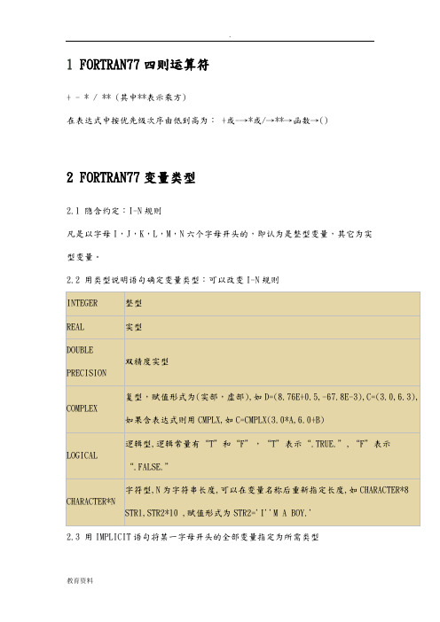
1 FORTRAN77四则运算符+ - * / ** (其中**表示乘方)在表达式中按优先级次序由低到高为： +或-→*或/→**→函数→()2 FORTRAN77变量类型2.1 隐含约定：I-N规则凡是以字母I，J，K，L，M，N六个字母开头的，即认为是整型变量，其它为实型变量。

2.2 用类型说明语句确定变量类型：可以改变I-N规则2.3 用IMPLICIT语句将某一字母开头的全部变量指定为所需类型如 IMPLICIT REAL (I,J)三种定义的优先级别由低到高顺序为：I-N规则→IMPLICIT语句→类型说明语句，因此，在程序中IMPLICIT语句应放在类型说明语句之前。

2.4 数组的说明与使用使用I-N规则时用DIMENSION说明数组，也可在定义变量类型同时说明数组，说明格式为：数组名(下标下界,下标上界），也可省略下标下界，此时默认为1，例：DIMENSION IA(0:9),ND(80:99),W(3,2),NUM(-1:0),A(0:2,0:1,0:3)REAL IA(10),ND(80:99)使用隐含DO循环进行数组输入输出操作：例如WRITE(*,10) ('I=',I,'A=',A(I),I=1,10,2)10FORMAT(1X,5(A2,I2,1X,A2,I4))2.5 使用DATA语句给数组赋初值变量表中可出现变量名,数组名,数组元素名,隐含DO循环，但不许出现任何形式的表达式：例如DATA A,B,C/-1.0,-1.0,-1.0/DATA A/-1.0/,B/-1.0/,C/-1.0/DATA A,B,C/3*-1.0/CHARACTER*6 CHN(10)DATA CHN/10*' '/INTEGER NUM(1000)DATA (NUM(I),I=1,500)/500*0/,(NUM(I),I=501,1000)/500*1/3 FORTRAN77程序书写规则程序中的变量名，不分大小写；变量名称是以字母开头再加上1到5位字母或数字构成，即变更名字串中只有前6位有效；一行只能写一个语句；程序的第一个语句固定为PROGRAM 程序名称字符串某行的第１个字符至第５个字符位为标号区，只能书写语句标号或空着或注释内容；某行的第１个字符为Ｃ或＊号时，则表示该行为注释行，其后面的内容为注释内容；某行的第６个字符位为非空格和非０字符时，则该行为上一行的续行，一个语句最多可有19个续行；某行的第７至７２字符位为语句区，语句区内可以任加空格以求美观；某行的第７３至８０字符位为注释区，８０字符位以后不能有内容。

Simufact Additive 是一款专为金属3D打印工艺设计的仿真软件，它可以帮助用户模拟和优化整个3D打印过程。

该软件包含了丰富的功能和工具，使用户能够更加准确地预测零件的变形、残余应力以及其他关键的制造过程参数。

本文将从以下几个方面介绍Simufact Additive 的手册，帮助读者更好地了解和使用这款软件。

一、Simufact Additive 手册的结构Simufact Additive 手册按照基本操作、高级建模、工作流程等方面对软件进行了系统的介绍和说明。

在基本操作部分，手册详细介绍了软件的安装、启动、基本界面、操作步骤等内容，为用户提供了一系列详细的操作指南和截图示例。

在高级建模部分，手册着重介绍了软件中的一些高级建模功能和技巧，如建立模型、设置材料属性、定义工艺参数等内容。

手册还对软件的工作流程进行了详细的介绍，帮助用户更好地掌握软件的整体使用方法。

二、Simufact Additive 手册的特点和优势Simufact Additive 手册在内容和结构上均具有一些明显的特点和优势。

手册内容全面、系统，覆盖了软件的各个方面，内容详实、易懂，为读者提供了一站式的学习和使用指南。

手册中的众多示例和实例，使得读者能够更加直观地理解软件的操作方法和技巧，提高了手册的可读性和实用性。

手册还设置了丰富的案例分析和实际应用，帮助用户将理论知识与实际工程应用相结合，提高了手册的实用性和指导性。

三、Simufact Additive 手册的使用方法和建议在阅读Simufact Additive 手册时，建议读者根据自己的实际情况和需求，有序地查阅手册内容，先从基本操作部分开始，逐步深入高级建模和工作流程等部分。

建议读者在阅读中积极参与实践操作，结合手册中的示例和案例，实际操作软件，加深对软件功能和操作方法的理解。

建议读者在阅读过程中及时记录问题和疑惑，积极向同行、专家或冠方交流，以便及时解决遇到的困难和问题。

fortran 简明教程Fortran是世界上最早的高级程序设计语言之一，广泛应用于科学计算、工程和数值分析等领域。

以下是Fortran的简明教程：1. 程序结构：一个Fortran程序由不同的程序单元组成，包括主程序、子程序和模块等。

每个程序单元都以END结束。

主程序是程序的入口点，可以包含变量声明、执行语句和控制语句等。

子程序可以包含函数和子例程，用于执行特定的任务。

模块用于提供程序中的公共代码和数据。

2. 变量声明：在Fortran中，变量必须先声明后使用。

变量类型包括整数型、实数型、字符型等。

例如，声明一个整数型变量可以这样写：INTEGER :: x3. 执行语句：执行语句用于控制程序的流程和执行顺序。

Fortran提供了多种控制语句，如IF语句、DO循环、WHILE循环等。

例如，使用IF语句进行条件判断：IF (x > 0) THEN y = x x ELSE y = -x x END IF4. 输入输出：Fortran提供了基本的输入输出功能。

可以使用READ语句从标准输入读取数据，使用WRITE语句将数据输出到标准输出。

例如，读取一个实数并输出到屏幕：READ(,) x WRITE(,) x5. 数组和矩阵：Fortran支持一维和多维数组，以及矩阵运算。

例如，声明一个二维实数数组并赋值：REAL :: A(3,3) A =RESHAPE((/1,2,3,4,5,6,7,8,9/), (/3,3/))6. 子程序和模块：子程序可以用于封装特定的功能或算法，并在主程序中调用。

模块可以包含公共的函数、子例程和变量等，用于提供可重用的代码和数据。

7. 调试和优化：Fortran提供了多种调试工具和技术，如断点、单步执行、变量监视等。

还可以使用性能分析工具来检查程序的性能瓶颈并进行优化。

以上是Fortran的简明教程，希望能帮助您快速入门Fortran编程。