推荐-Broyden方法求解非线性方程组的Matlab实现 精品

broyden 法-回复关于Broyden法的原理和应用。

Broyden法是一种迭代法，用于求解非线性方程组的数值解。

它是通过近似逆Jacobi矩阵的方法，在每一次迭代中更新Jacobi矩阵的逆矩阵，从而更新模型中的解向量。

该方法被广泛应用于各个领域，包括数学建模、物理学、工程学等。

Broyden法的原理是基于牛顿法和拟牛顿法的思想。

在牛顿法中，我们通过不断迭代求解线性化的方程组来逼近方程的解。

拟牛顿法则是通过近似Hessian矩阵的逆矩阵来更新解向量。

Broyden法则是基于拟牛顿法，但使用Jacobi矩阵的逆矩阵（即Broyden矩阵）来更新解向量。

假设我们要求解的非线性方程组为F(x) = 0，其中x为未知量向量，F(x)为方程组的函数向量。

初始解向量x0可以通过任意方法选择。

使用Broyden法求解该方程组的过程如下：1. 初始化：选择初始解向量x0和对应的函数向量F(x0)，并计算初始Jacobi矩阵的逆矩阵B0。

2. 迭代计算：对于每一次迭代k，假设我们已经有了解向量xk和对应的函数向量F(xk)。

我们首先计算增量向量dk，使得F(xk+dk) = 0。

具体计算方法为：dk = -Bk * F(xk)。

其中Bk为Jacobi矩阵的逆矩阵。

3. 更新解向量：通过计算得到的增量向量dk更新解向量xk+1 = xk + dk。

4. 更新Jacobi矩阵的逆矩阵：通过计算得到的解向量增量dk和函数向量增量dF = F(xk+1) - F(xk)来更新Jacobi矩阵的逆矩阵Bk+1 = Bk + (dF - Bk * dk) * dk' / (dk' * dk)。

5. 判断停止条件：如果满足停止条件（如收敛到某个精度要求或达到最大迭代次数），则停止迭代。

否则，回到步骤2。

Broyden法的优点在于它的收敛速度相对较快，同时也不需要计算Hessian矩阵的逆矩阵。

这使得Broyden法在求解大型非线性方程组时非常适用。

MATLAB中的非线性优化算法详解在计算机科学和工程领域，非线性优化是一个非常重要的问题。

它涉及到在给定一些约束条件下，寻找使得目标函数取得最优值的变量取值。

MATLAB作为一种强大的数值计算工具，提供了多种非线性优化算法来解决这个问题。

本文将详细介绍一些常用的非线性优化算法，并探讨它们的特点和适用场景。

1. 数学背景在介绍非线性优化算法之前，我们先来了解一下非线性优化的基本数学背景。

一个非线性优化问题可以表示为以下形式：minimize f(x)subject to g(x) ≤ 0h(x) = 0其中，f(x)是目标函数，g(x)是不等式约束条件，h(x)是等式约束条件。

x是优化变量。

目标是找到x使得f(x)取得最小值，并且满足约束条件。

2. 黄金分割法黄金分割法是一种经典的非线性优化算法。

它基于一个简单的原则：将搜索区间按照黄金分割比例分为两段，并选择一个更优的区间进行下一次迭代。

该算法的思想简单明了，但是它的收敛速度比较慢，特别是对于高维问题。

因此，该算法在实际应用中较少使用。

3. 拟牛顿法拟牛顿法是一类比较常用的非线性优化算法。

它通过近似目标函数的梯度信息来进行迭代优化。

拟牛顿法的核心思想是构造一个Hessian矩阵的近似矩阵，来更新搜索方向和步长。

其中，DFP算法和BFGS算法是拟牛顿法的两种典型实现。

DFP算法是由Davidon、Fletcher和Powell于1959年提出的，它通过不断迭代来逼近最优解。

该算法的优点是收敛性比较好，但是它需要存储中间结果，占用了较多的内存。

BFGS算法是由Broyden、Fletcher、Goldfarb和Shanno于1970年提出的。

它是一种变种的拟牛顿法，通过逼近Hessian矩阵的逆矩阵来求解最优解。

BFGS算法在存储方面比DFP算法更加高效，但是它的计算复杂度相对较高。

4. 信赖域法信赖域法是一种迭代优化算法，用于解决非线性优化问题。

它将非线性优化问题转化为一个二次规划问题，并通过求解这个二次规划问题来逼近最优解。

1.fsolve求解非线性方程组方程：F(x)=0x是一个向量，F(x)是该向量的函数向量，返回向量值2.语法x = fsolve(fun,x0)x = fsolve(fun,x0,options)[x,fval] = fsolve(fun,x0)[x,fval,exitflag] = fsolve(...)[x,fval,exitflag,output] = fsolve(...)[x,fval,exitflag,output,jacobian] = fsolve(...)3.描述fsolve 用于寻找非线性系统方程组的零点。

x = fsolve(fun,xO)以x0为初始值，努力寻找在fun中描述的方程组。

x = fsolve(fun,xO,options)以x0为初始值，按照指定的优化设置“options努力寻找在fun 中描述的方程组。

使用optimset 设置这些选项。

[x,fval] = fsolve(fun,xO)返回在解x处的目标函数fun的值[x,fval,exitflag] = fsolve(...)返回exitflag 表示退出条件。

[x,fval,exitflag,output] = fsolve(...)返回output 结构，该结构包含了优化信息。

[x,fval,exitflag,output,jacobian]二fsolve(…)返回在解x 处的Jacobian 函数。

4.输入参数4.1."fun非线性系统方程。

它是一个函数，以x作为输入，返回向量F。

函数fun可以被指定为一个M 文件函数的函数句柄。

x = fsolve(@myfun,x0)这里的myfun 是一个matlab 函数，形如：function F = myfun(x)F = ...% Compute function values at xfun 也可以是一个异步函数的函数句柄：x = fsolve(@(x)sin(x.*x),x0);若用户定义的值为矩阵，则会被自动转换为向量。

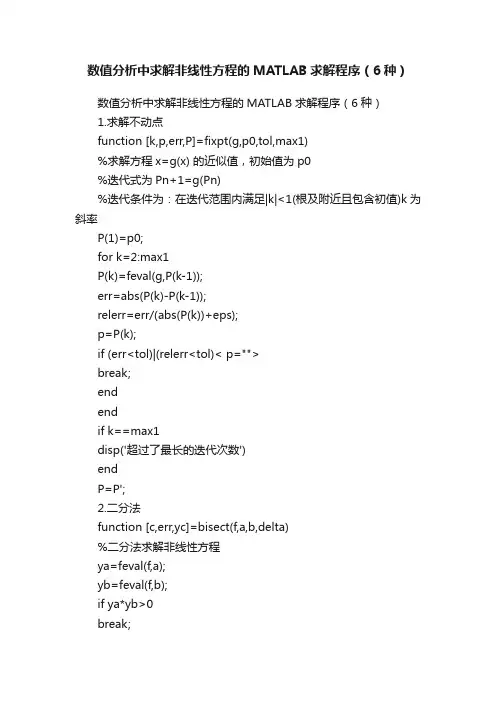
数值分析中求解非线性方程的MATLAB求解程序（6种）数值分析中求解非线性方程的MATLAB求解程序（6种）1.求解不动点function [k,p,err,P]=fixpt(g,p0,tol,max1)%求解方程x=g(x) 的近似值，初始值为p0%迭代式为Pn+1=g(Pn)%迭代条件为：在迭代范围内满足|k|<1(根及附近且包含初值)k为斜率P(1)=p0;for k=2:max1P(k)=feval(g,P(k-1));err=abs(P(k)-P(k-1));relerr=err/(abs(P(k))+eps);p=P(k);if (err<tol)|(relerr<tol)< p="">break;endendif k==max1disp('超过了最长的迭代次数')endP=P';2.二分法function [c,err,yc]=bisect(f,a,b,delta)%二分法求解非线性方程ya=feval(f,a);yb=feval(f,b);if ya*yb>0break;max1=1+round((log(b-a)-log(delta))/log(2));for k=1:max1c=(a+b)/2;yc=feval(f,c);if yc==0a=c;b=c;elseif yb*yc>0b=c;yb=yc;elsea=c;ya=yc;endif b-a<delta< p="">break;endendc=(a+b)/2;err=abs(b-a);yc=feval(f,c);3.试值法function [c,err,yc]=regula(f,a,b,delta,epsilon,max1) %试值法求解非线性方程%f(a)和飞(b)异号ya=feval(f,a);yb=feval(f,b);if ya*yb>0disp('Note:f(a)*f(b)>0');for k=1:max1dx=yb*(b-a)/(yb-ya);c=b-dx;ac=c-a;yc=feval(f,c);if yc==0break;elseif yb*yc>0b=c;yb=yc;elsea=c;ya=yc;enddx=min(abs(dx),ac);if abs(dx)<delta|abs(yc)<epsilon< p="">break;endendc;err=abs(b-a)/2;yc=feval(f,c);4.求解非线性方程根的近似位置function R=approot(X,epsilon)%求解根近似位置%为了粗估算方程f(x)=0在区间[a,b]的根的位置，%使用等间隔采样点(xk,f(xk))和如下的评定准则：%f(xk-1)与f(xk)符号相反，%或者|f(xk)|足够小且曲线y=f(x)的斜率在%(xk,f(xk))附近改变符号。

B r o y d e n方法求解非线性方程组的M a t l a b实现-CAL-FENGHAI.-(YICAI)-Company One1Broyden方法求解非线性方程组的Matlab实现注：matlab代码来自网络，仅供学习参考。

1.把以下代码复制在一个.m文件上function [sol, it_hist, ierr] = brsola(x,f,tol, parms)% Broyden's Method solver, globally convergent% solver for f(x) = 0, Armijo rule, one vector storage%% This code comes with no guarantee or warranty of any kind.%% function [sol, it_hist, ierr] = brsola(x,f,tol,parms)%% inputs:% initial iterate = x% function = f% tol = [atol, rtol] relative/absolute% error tolerances for the nonlinear iteration% parms = [maxit, maxdim]% maxit = maxmium number of nonlinear iterations% default = 40% maxdim = maximum number of Broyden iterations% before restart, so maxdim-1 vectors are% stored% default = 40%% output:% sol = solution% it_hist(maxit,3) = scaled l2 norms of nonlinear residuals% for the iteration, number function evaluations,% and number of steplength reductions% ierr = 0 upon successful termination% ierr = 1 if after maxit iterations% the termination criterion is not satsified.% ierr = 2 failure in the line search. The iteration% is terminated if too many steplength reductions% are taken.%%% internal parameter:% debug = turns on/off iteration statistics display as% the iteration progresses%% alpha = , parameter to measure sufficient decrease%% maxarm = 10, maximum number of steplength reductions before % failure is reported%% set the debug parameter, 1 turns display on, otherwise off%debug=1;%% initialize it_hist, ierr, and set the iteration parameters%ierr = 0; maxit=40; maxdim=39;it_histx=zeros(maxit,3);maxarm=10;%if nargin == 4maxit=parms(1); maxdim=parms(2)-1;endrtol=tol(2); atol=tol(1); n = length(x); fnrm=1; itc=0; nbroy=0;%% evaluate f at the initial iterate% compute the stop tolerance%f0=feval(f,x);fc=f0;fnrm=norm(f0)/sqrt(n);it_hist(itc+1)=fnrm;it_histx(itc+1,1)=fnrm; it_histx(itc+1,2)=0; it_histx(itc+1,3)=0;fnrmo=1;stop_tol=atol + rtol*fnrm;outstat(itc+1, :) = [itc fnrm 0 0];%% terminate on entry%if fnrm < stop_tolsol=x;returnend%% initialize the iteration history storage matrices%stp=zeros(n,maxdim);stp_nrm=zeros(maxdim,1);lam_rec=ones(maxdim,1);%% Set the initial step to -F, compute the step norm%lambda=1;stp(:,1) = -fc;stp_nrm(1)=stp(:,1)'*stp(:,1);%% main iteration loop%while(itc < maxit)%nbroy=nbroy+1;%% keep track of successive residual norms and% the iteration counter (itc)%fnrmo=fnrm; itc=itc+1;%% compute the new point, test for termination before% adding to iteration history%xold=x; lambda=1; iarm=0; lrat=.5; alpha=;x = x + stp(:,nbroy);fc=feval(f,x);fnrm=norm(fc)/sqrt(n);ff0=fnrmo*fnrmo; ffc=fnrm*fnrm; lamc=lambda;%%% Line search, we assume that the Broyden direction is an% ineact Newton direction. If the line search fails to% find sufficient decrease after maxarm steplength reductions % brsola returns with failure.%% Three-point parabolic line search%while fnrm >= (1 - lambda*alpha)*fnrmo && iarm < maxarm % lambda=lambda*lrat;if iarm==0lambda=lambda*lrat;elselambda=parab3p(lamc, lamm, ff0, ffc, ffm);endlamm=lamc; ffm=ffc; lamc=lambda;x = xold + lambda*stp(:,nbroy);fc=feval(f,x);fnrm=norm(fc)/sqrt(n);ffc=fnrm*fnrm;iarm=iarm+1;end%% set error flag and return on failure of the line search%if iarm == maxarmdisp('Line search failure in brsola ')ierr=2;it_hist=it_histx(1:itc+1,:);sol=xold;return;end%% How many function evaluations did this iteration require %it_histx(itc+1,1)=fnrm;it_histx(itc+1,2)=it_histx(itc,2)+iarm+1;if(itc == 1) it_histx(itc+1,2) = it_histx(itc+1,2)+1; end;it_histx(itc+1,3)=iarm;%% terminate%if fnrm < stop_tolsol=x;rat=fnrm/fnrmo;outstat(itc+1, :) = [itc fnrm iarm rat];it_hist=it_histx(1:itc+1,:);% it_hist(itc+1)=fnrm;if debug==1disp(outstat(itc+1,:))endreturnend%%% modify the step and step norm if needed to reflect the line % search%lam_rec(nbroy)=lambda;if lambda ~= 1stp(:,nbroy)=lambda*stp(:,nbroy);stp_nrm(nbroy)=lambda*lambda*stp_nrm(nbroy);end%%% it_hist(itc+1)=fnrm;rat=fnrm/fnrmo;outstat(itc+1, :) = [itc fnrm iarm rat];if debug==1disp(outstat(itc+1,:))end%%% if there's room, compute the next search direction and step norm and % add to the iteration history%if nbroy < maxdim+1z=-fc;if nbroy > 1for kbr = 1:nbroy-1ztmp=stp(:,kbr+1)/lam_rec(kbr+1);ztmp=ztmp+(1 - 1/lam_rec(kbr))*stp(:,kbr);ztmp=ztmp*lam_rec(kbr);z=z+ztmp*((stp(:,kbr)'*z)/stp_nrm(kbr));endend%% store the new search direction and its norm%a2=-lam_rec(nbroy)/stp_nrm(nbroy);a1=1 - lam_rec(nbroy);zz=stp(:,nbroy)'*z;a3=a1*zz/stp_nrm(nbroy);a4=1+a2*zz;stp(:,nbroy+1)=(z-a3*stp(:,nbroy))/a4;stp_nrm(nbroy+1)=stp(:,nbroy+1)'*stp(:,nbroy+1);%%%else%% out of room, time to restart%stp(:,1)=-fc;stp_nrm(1)=stp(:,1)'*stp(:,1);nbroy=0;%%%end%% end whileend%% We're not supposed to be here, we've taken the maximum% number of iterations and not terminated.%sol=x;it_hist=it_histx(1:itc+1,:);ierr=1;if debug==1disp(' outstat')endfunction lambdap = parab3p(lambdac, lambdam, ff0, ffc, ffm)% Apply three-point safeguarded parabolic model for a line search. %% This code comes with no guarantee or warranty of any kind.%% function lambdap = parab3p(lambdac, lambdam, ff0, ffc, ffm)%% input:% lambdac = current steplength% lambdam = previous steplength% ff0 = value of \| F(x_c) \|^2% ffc = value of \| F(x_c + \lambdac d) \|^2% ffm = value of \| F(x_c + \lambdam d) \|^2%% output:% lambdap = new value of lambda given parabolic model%% internal parameters:% sigma0 = .1, sigma1=.5, safeguarding bounds for the linesearch %%% set internal parameters%sigma0=.1; sigma1=.5;%% compute coefficients of interpolation polynomial%% p(lambda) = ff0 + (c1 lambda + c2 lambda^2)/d1%% d1 = (lambdac - lambdam)*lambdac*lambdam < 0% so if c2 > 0 we have negative curvature and default to% lambdap = sigam1 * lambda%c2 = lambdam*(ffc-ff0)-lambdac*(ffm-ff0);if c2 >= 0lambdap = sigma1*lambdac; returnendc1=lambdac*lambdac*(ffm-ff0)-lambdam*lambdam*(ffc-ff0);lambdap=-c1*.5/c2;if (lambdap < sigma0*lambdac) lambdap=sigma0*lambdac; endif (lambdap > sigma1*lambdac) lambdap=sigma1*lambdac; end2.应用举例把以下代码复制在command 窗口中x=[1 2 3]’;f=@(x)[3*x(1)-cos(x(2)*x(3))-1/2;x(1)^2-81*(x(2)+^2+sin(x(3))+;exp(-x(1)*x(2))+20*x(3)+(10*pi-3)/3;];tol=[3,-5];[sol, it_hist, ierr] = brsola(x,f,tol)说明：以上应用举例只是给出了上文中代码的一个应用实例，具体能否得到方程的满意数值解还需要进一步调节初始给的x和tol的值。

matlab 求解不等方程组求解不等方程组是数学中一个常见的问题，而Matlab作为一种功能强大的计算软件，可以方便地解决这类问题。

本文将介绍如何使用Matlab来求解不等方程组的方法和步骤。

我们需要明确什么是不等方程组。

不等方程组是指方程组中包含不等式的一种形式。

例如：```x + y >= 52x - y <= 10```这是一个简单的不等方程组，其中包含了两个不等式。

求解不等方程组的目标是找到满足所有不等式的变量取值。

在Matlab中，可以使用线性规划工具箱来求解不等方程组。

线性规划是一种优化问题，目标是找到一组变量的取值，使得目标函数的值最大或最小，同时满足一组线性不等式和等式约束。

我们需要定义不等方程组。

在Matlab中，可以使用矩阵和向量的形式来表示不等方程组。

例如，上述的不等方程组可以表示为：```A = [1 1; 2 -1];b = [5; 10];```其中，矩阵A表示不等式的系数，向量b表示不等式的右边常数。

接下来，我们需要定义目标函数和变量的取值范围。

在Matlab中，可以使用linprog函数来求解线性规划问题。

该函数的语法如下：```x = linprog(f, A, b, Aeq, beq, lb, ub)```其中，f是目标函数的系数向量，A和b是不等式约束的矩阵和向量，Aeq和beq是等式约束的矩阵和向量，lb和ub是变量的下界和上界。

对于不等方程组，我们可以将目标函数设置为一个常数向量，表示我们只关心满足不等式的变量取值。

同时，我们需要设置变量的上下界，表示变量的取值范围。

假设我们要求解的不等方程组为：```x + y >= 52x - y <= 10```我们可以将目标函数设置为 f = [0; 0]，表示我们只关心满足不等式的变量取值，不关心变量的具体取值。

同时，我们可以设置变量的上下界为lb = [-inf; -inf]，ub = [inf; inf]，表示变量的取值范围为无穷大。

第7章 求解非线性方程7.1 多项式运算在MATLAB 中的实现一、多项式的表达n 次多项式表达为：n a +⋯⋯++=x a x a x a p(x)1-n 1-n 1n 0，是n+1项之和 在MATLAB 中，n 次多项式可以用n 次多项式系数构成的长度为n+1的行向量表示[a0, a1,……an-1,an]二、多项式的加减运算 设有两个多项式na +⋯⋯++=x a x a x a p1(x)1-n 1-n 1n 0和m b +⋯⋯++=x b x b x b p2(x)1-m 1-m 1m 0。

它们的加减运算实际上就是它们的对应系数的加减运算。

当它们的次数相同时，可以直接对多项式的系数向量进行加减运算。

当它们的次数不同时，应该把次数低的多项式无高次项部分用0系数表示。

例2 计算()()1635223-+++-x x x xa=[1, -2, 5, 3]; b=[0, 0, 6, -1]; c=a+b例 3 设()6572532345++-+-=x x x x x x f ，()3532-+=x x x g ，求f(x)+g(x)f=[3, -5, 2, -7, 5, 6]; g=[3, 5, -3]; g1=[0, 0, 0, g];%为了和f 的次数找齐f+g1, f-g1三、多项式的乘法运算conv(p1,p2)例4 在上例中，求f(x)*g(x)f=[3, -5, 2, -7, 5, 6]; g=[3, 5, -3]; conv(f, g)四、多项式的除法运算[Q, r]=deconv(p1, p2)表示p1除以p2，给出商式Q(x)，余式r(x)。

Q,和r 仍为多项式系数向量 例4 在上例中，求f(x)/g(x)f=[3, -5, 2, -7, 5, 6]; g=[3, 5, -3]; [Q, r]=deconv(f, g) 五、多项式的导函数p=polyder(P)：求多项式P 的导函数 p=polyder(P,Q)：求P ·Q 的导函数[p,q]=polyder(P,Q)：求P/Q 的导函数，导函数的分子存入p ，分母存入q 。

broyden 法-回复什么是Broyden法？Broyden法是一种求解非线性方程组的数值方法，由英国数学家Charles George Broyden在1965年提出。

该方法通过使用一种迭代算法来逐步逼近方程组的解，而不需要计算每个迭代步骤的雅可比矩阵，从而提高计算效率。

Broyden法在科学和工程领域中被广泛应用，特别是在求解非线性优化问题和微分方程组中。

Broyden法的基本思想是使用迭代来改进解的逼近值。

假设我们有一个非线性方程组F(x) = 0，其中x是未知向量，F是向量函数。

初始迭代步骤中，我们需要给定一个初始逼近值x0，并计算对应的函数值F0 = F(x0)。

然后，我们需要计算一个初始的雅可比矩阵J0，它可以用任何一种方法计算得到，如有限差分法或解析方法。

迭代的过程中，我们需要更新逼近值x和函数值F，并计算一个近似的雅可比矩阵。

具体的步骤如下：步骤1：给定初始逼近值x0和函数值F0。

步骤2：计算初始雅可比矩阵J0。

步骤3：对于迭代步k，计算方程组的残差v：v = F(xk)。

步骤4：更新逼近值：xk+1 = xk - Jk^(-1) v。

步骤5：计算函数值的变化量：ΔF = F(xk+1) - F(xk)。

步骤6：通过更新逼近值的变化量和残差的变化量来计算新的雅可比矩阵：Jk+1 = Jk + (∆xk ⊗∆Fk) / (∆Fk^T ∆Fk) 。

步骤7：重复步骤3-6，直到满足收敛准则（例如，残差的绝对值小于给定阈值）。

Broyden法的核心是在每个迭代步骤中，通过使用上一步的雅可比矩阵和逼近值的变化量和函数值的变化量来计算新的雅可比矩阵。

这避免了在每个迭代步骤中重新计算雅可比矩阵，从而节省了计算时间和资源。

与其他求解非线性方程组的方法相比，Broyden法具有许多优点。

首先，它不需要计算雅可比矩阵的全局近似，而是通过迭代来逐步改进它。

这也意味着它不需要存储和更新完整的雅可比矩阵，从而减少了内存要求。