Stability, Accuracy, and Efficiency of Sequential Methods for Coupled Flow and Geomechanics
- 格式:pdf
- 大小:652.74 KB
- 文档页数:14

摘要定位是自动驾驶车辆自主导航技术的关键问题之一。
保持稳定、精确、实时的定位能够保证自动驾驶车辆行驶的安全。
自动驾驶车辆的定位方式主要有:基于全球卫星导航系统(Global Navigation Satellite System, GNSS)的定位方式,基于激光雷达点云地图匹配的定位方式等。
目前在自动驾驶领域,全球卫星导航系统是使用最广泛、应用最成熟的定位技术,自动驾驶车辆依靠GNSS定位技术能够在大多数场景下完成精确定位与导航,但仍然存在卫星信号被周边环境的建筑物和树木等障碍物遮挡导致定位失效或者偏移等状况。
目前为了提高定位精度,利用GNSS中的实时差分定位技术(Real-time Kinematic, RTK)结合惯性导航系统(Inertial Navigation System, INS)进行多传感器融合定位,以满足自动驾驶车辆高精度定位的需求。
但是,在复杂地形环境下对定位的干扰依然不可避免,因此在自动驾驶领域基于全球卫星导航系统的定位方式在地形环境复杂的场景下仍受到很大的限制。
车载激光雷达采集的点云地图不仅能够提供全方位的道路特征信息,同时,能够为自动驾驶车辆实现厘米级定位提供数据基础。
基于点云地图匹配的定位技术能够不受天气、地形等环境因素的影响,在定位测算中保持相互独立,在复杂环境下替代GNSS定位,为自动驾驶车辆的安全行驶提供保障。
为此,本文对基于点云地图匹配的定位技术进行研究,并对经典的点云匹配算法进行改进,对比不同算法在复杂环境下的定位精度和效率,验证基于点云地图匹配的定位技术的可行性。
本文的研究数据选取于目前国际上最大的自动驾驶场景数据集(KITTI)中的城市环境点云数据。
首先,对点云数据进行预处理,利用LOAM算法预先构建出点云地图,作为匹配定位实验的基础数据,利用PCL库中的滤波算法对点云数据中存在的噪声点进行过滤优化,增强匹配定位的稳定性;然后,分别利用迭代最近点(Iterative Closest Points,ICP)算法和正态分布变换(Normal Distribution Transform,NDT)算法进行单帧点云与点云地图的匹配定位实验,分析两种算法的稳定性、精度以及效率;最后,在当前完成匹配定位的基础上进行研究和算法改进,利用Gauss-Newton 法改进ICP算法,同时利用K-D树加速查找对应点,并且和NDT算法进行集成,定义为NDT-ICP算法,进行匹配定位实验。
Robust ControlRobust control is a critical aspect of engineering that deals with designing systems that can perform effectively in the presence of uncertainties and variations. It is essential for ensuring the stability and performance of complex systems in various industries, including aerospace, automotive, and manufacturing. Robust control techniques aim to account for uncertainties in the system dynamics, external disturbances, and variations in operating conditions to ensure reliable and predictable system behavior. One of the key challenges in robust control is dealing with uncertainties in system parameters. These uncertainties can arise due to variations in component properties, environmental conditions, or modeling errors. Robust control techniques, such as H-infinity control and mu-synthesis, provide a systematic framework for designing controllers that can guarantee stability and performance in the presence of these uncertainties. By considering the worst-case scenarios and optimizing the system performance under these conditions, robust control techniques can enhance the reliability and robustness of the system. Another important aspect of robust control is handling external disturbances that can affect the system's performance. External disturbances, such as wind gusts in aerospace systems or road irregularities in automotive systems, can introduce uncertainties that can destabilize the system if not properly addressed. Robust control techniques, such as disturbance rejection control and adaptive control, enable the system to mitigate the effects of external disturbances and maintain stable performance under varying operating conditions. In addition to uncertainties and disturbances, robust control also plays a crucial role in ensuring the safety and reliability of systems in critical applications. For example, in automotive systems, robust control techniques are essential for designing controllers that can prevent accidents and ensure passenger safety under extreme driving conditions. In aerospace systems, robust control is vital for maintaining the stability of aircraft during flight and landing, even in the presence of uncertainties and disturbances. Moreover, robust control techniques are also essential for enhancing the performance of systems in terms of speed, accuracy, and efficiency. By optimizing the control strategies to account for uncertainties and disturbances, robust control can improve the overall systemperformance and achieve better control objectives. This is particularly importantin high-performance applications, such as robotic systems, where precise controlis essential for accomplishing complex tasks with accuracy and reliability. Overall, robust control is a critical aspect of engineering that addresses the challenges of uncertainties, disturbances, and variations in system dynamics. By applying robust control techniques, engineers can design systems that are reliable, stable, and efficient under varying operating conditions. From aerospace and automotive systems to manufacturing and robotics, robust control plays a vitalrole in ensuring the safety, reliability, and performance of complex engineering systems.。
先张法预应力混凝土构件的生产流程1.混凝土搅拌车将混凝土原材料运送至混凝土搅拌站。
The concrete mixer truck transports the raw materials of concrete to the concrete mixing station.2.在搅拌站,混凝土材料被充分搅拌成均匀的混凝土浆料。
At the mixing station, the concrete materials are thoroughly mixed into a uniform concrete slurry.3.通过混凝土泵,混凝土浆料被送入预应力构件的模具中。
The concrete slurry is pumped into the mold of the pre-stressed component.4.模具中的混凝土浆料在模具中进行振实和养护。
The concrete slurry in the mold is compacted and cured in the mold.5.完成振实和养护后,模具中的混凝土构件被取出并进行表面修整。
After compaction and curing, the concrete component in the mold is taken out and the surface is finished.6.随后的预应力加工,包括预应力筋的预埋和张拉。
The subsequent pre-stressing process includes the embedding and tensioning of pre-stressed tendons.7.预应力筋通过张拉设备进行张拉,并进行锚固。
The pre-stressed tendons are tensioned by the tensioning equipment and anchored.8.进行预应力筋张拉后,混凝土构件的预应力效应得以形成。
矩阵逆学习资料woodbury公式关于矩阵逆的补充学习资料:Woodbury matrix identity本⽂来⾃维基百科。
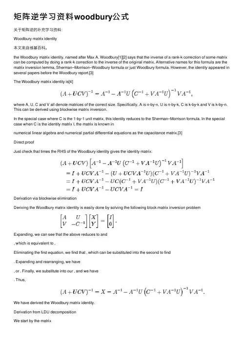
the Woodbury matrix identity, named after Max A. Woodbury[1][2] says that the inverse of a rank-k correction of some matrix can be computed by doing a rank-k correction to the inverse of the original matrix. Alternative names for this formula are the matrix inversion lemma, Sherman–Morrison–Woodbury formula or just Woodbury formula. However, the identity appeared in several papers before the Woodbury report.[3]The Woodbury matrix identity is[4]where A, U, C and V all denote matrices of the correct size. Specifically, A is n-by-n, U is n-by-k, C is k-by-k and V is k-by-n. This can be derived using blockwise matrix inversion.In the special case where C is the 1-by-1 unit matrix, this identity reduces to the Sherman–Morrison formula. In the special case when C is the identity matrix I, the matrix is known innumerical linear algebra and numerical partial differential equations as the capacitance matrix.[3]Direct proofJust check that times the RHS of the Woodbury identity gives the identity matrix:Derivation via blockwise eliminationDeriving the Woodbury matrix identity is easily done by solving the following block matrix inversion problemExpanding, we can see that the above reduces to and, which is equivalent to .Eliminating the first equation, we find that , which can be substituted into the second to find. Expanding and rearranging, we have, or . Finally, we substitute into our , and we have. Thus,We have derived the Woodbury matrix identity.Derivation from LDU decompositionWe start by the matrixBy eliminating the entry under the A (given that A is invertible) we getLikewise, eliminating the entry above C givesNow combining the above two, we getMoving to the right side giveswhich is the LDU decomposition of the block matrix into an upper triangular, diagonal, and lower triangular matrices.Now inverting both sides givesWe could equally well have done it the other way (provided that C is invertible) i.e.Now again inverting both sides,Now comparing elements (1,1) of the RHS of (1) and (2) above gives the Woodbury formulaApplicationsThis identity is useful in certain numerical computations where A?1has already been computed and it is desired to compute (A+ UCV)?1. With the inverse of A available, it is only necessary tofind the inverse of C?1+ VA?1U in order to obtain the result using the right-hand side of the identity. If C has a much smaller dimension than A, this is more efficient than inverting A+ UCV directly. A common case is finding the inverse of a low-rank update A+ UCV of A (where U only has a few columns and V only a few rows), or finding an approximation of the inverse of the matrix A+ B where the matrix can be approximated by a low-rank matrix UCV, for example using the singular value decomposition.This is applied, e.g., in the Kalman filter and recursive least squares methods, to replace the parametric solution, requiring inversion of a state vector sized matrix, with a condition equations based solution. In case of the Kalman filter this matrix has the dimensions of the vector of observations, i.e., as small as 1 in case only one new observation is processed at a time. This significantly speeds up the often real time calculations of the filter.See also:Sherman–Morrison formulaInvertible matrixSchur complementMatrix determinant lemma, formula for a rank-k update to a determinantBinomial inverse theorem; slightly more general identity. Notes:1.Jump up ^ Max A. Woodbury, Inverting modified matrices, MemorandumRept. 42, Statistical Research Group, Princeton University,Princeton, NJ, 1950, 4pp MR381362.Jump up ^ Max A. Woodbury, The Stability of Out-Input Matrices.Chicago, Ill., 1949. 5 pp. MR325643.^ Jump up to: a b Hager, William W. (1989). "Updating the inverse of amatrix". SIAM Review31 (2): 221–239. doi:10.1137/1031049.JSTOR2030425. MR997457.4.Jump up ^Higham, Nicholas (2002). Accuracy and Stability ofNumerical Algorithms (2nd ed.). SIAM. p. 258. ISBN978-0-89871-521-7. MR1927606.Press, WH; Teukolsky, SA; Vetterling, WT; Flannery, BP (2007), "Section 2.7.3. Woodbury Formula", Numerical Recipes: The Artof Scientific Computing (3rd ed.), New York: CambridgeUniversity Press, ISBN978-0-521-88068-8External links:Some matrix identitiesWeisstein, Eric W., "Woodbury formula", MathWorld.src="///doc/2742834010661ed9ad51f3e6.html /wiki/Special:CentralAutoLogin/start?type=1x1" alt="" title="" width="1" height="1" style="border: none; position: absolute;" />Retrieved from"/doc/2742834010661ed9ad51f3e6.html /w/index.php?title=Woodbury_matrix_identity&oldid=627695139"Categories:Linear algebraLemmasSherman–Morrison formula(来⾃维基百科。
内径8外径15厚度5的轴承型号及规格1.这款轴承的型号是6808,规格为内径8mm,外径15mm,厚度5mm。
This bearing model is 6808, with specifications of inner diameter 8mm, outer diameter 15mm, and thickness 5mm.2.轴承是由内圈、外圈、滚动体和保持架组成的。
The bearing is composed of inner ring, outer ring, rolling elements, and cage.3. 6808型轴承适用于高速旋转和高精度传动装置。
The 6808 bearing is suitable for high-speed rotation and high-precision transmission devices.4.轴承的材质通常为铬钢,具有良好的耐磨性和耐腐蚀性。
The material of the bearing is usually chrome steel, which has good wear resistance and corrosion resistance.5.这款轴承能够承受较大的径向和轴向载荷。
This bearing can withstand large radial and axial loads.6.装配时应注意保持轴承清洁,并且使用适量的润滑脂。
When assembling, care should be taken to keep the bearing clean and use the appropriate amount of grease.7.轴承在运转过程中应避免受到冲击和震动,以免影响其使用寿命。
Bearings should avoid impact and vibration duringoperation to avoid affecting their service life.8. 6808型轴承广泛应用于摩托车、电机、汽车和其他机械设备中。

HPLC ASSAY with DETERMINATION OF META-FLUOXETINE HCl.ANALYTICAL METHOD VALIDATION10 and 20mg Fluoxetine Capsules HPLC DeterminationFLUOXETINE HClC17H18F3NO•HClM.W. = 345.79CAS — 59333-67-4STABILITY INDICATINGA S S A Y V A L I D A T I O NMethod is suitable for:ýIn-process controlþProduct ReleaseþStability indicating analysis (Suitability - US/EU Product) CAUTIONFLUOXETINE HYDROCHLORIDE IS A HAZARDOUS CHEMICAL AND SHOULD BE HANDLED ONLY UNDER CONDITIONS SUITABLE FOR HAZARDOUS WORK.IT IS HIGHLY PRESSURE SENSITIVE AND ADEQUATE PRECAUTIONS SHOULD BE TAKEN TO AVOID ANY MECHANICAL FORCE (SUCH AS GRINDING, CRUSHING, ETC.) ON THE POWDER.ED. N0: 04Effective Date:APPROVED::HPLC ASSAY with DETERMINATION OF META-FLUOXETINE HCl.ANALYTICAL METHOD VALIDATION10 and 20mg Fluoxetine Capsules HPLC DeterminationTABLE OF CONTENTS INTRODUCTION........................................................................................................................ PRECISION............................................................................................................................... System Repeatability ................................................................................................................ Method Repeatability................................................................................................................. Intermediate Precision .............................................................................................................. LINEARITY................................................................................................................................ RANGE...................................................................................................................................... ACCURACY............................................................................................................................... Accuracy of Standard Injections................................................................................................ Accuracy of the Drug Product.................................................................................................... VALIDATION OF FLUOXETINE HCl AT LOW CONCENTRATION........................................... Linearity at Low Concentrations................................................................................................. Accuracy of Fluoxetine HCl at Low Concentration..................................................................... System Repeatability................................................................................................................. Quantitation Limit....................................................................................................................... Detection Limit........................................................................................................................... VALIDATION FOR META-FLUOXETINE HCl (POSSIBLE IMPURITIES).................................. Meta-Fluoxetine HCl linearity at 0.05% - 1.0%........................................................................... Detection Limit for Fluoxetine HCl.............................................................................................. Quantitation Limit for Meta Fluoxetine HCl................................................................................ Accuracy for Meta-Fluoxetine HCl ............................................................................................ Method Repeatability for Meta-Fluoxetine HCl........................................................................... Intermediate Precision for Meta-Fluoxetine HCl......................................................................... SPECIFICITY - STABILITY INDICATING EVALUATION OF THE METHOD............................. FORCED DEGRADATION OF FINISHED PRODUCT AND STANDARD..................................1. Unstressed analysis...............................................................................................................2. Acid Hydrolysis stressed analysis..........................................................................................3. Base hydrolysis stressed analysis.........................................................................................4. Oxidation stressed analysis...................................................................................................5. Sunlight stressed analysis.....................................................................................................6. Heat of solution stressed analysis.........................................................................................7. Heat of powder stressed analysis.......................................................................................... System Suitability stressed analysis.......................................................................................... Placebo...................................................................................................................................... STABILITY OF STANDARD AND SAMPLE SOLUTIONS......................................................... Standard Solution...................................................................................................................... Sample Solutions....................................................................................................................... ROBUSTNESS.......................................................................................................................... Extraction................................................................................................................................... Factorial Design......................................................................................................................... CONCLUSION...........................................................................................................................ED. N0: 04Effective Date:APPROVED::HPLC ASSAY with DETERMINATION OF META-FLUOXETINE HCl.ANALYTICAL METHOD VALIDATION10 and 20mg Fluoxetine Capsules HPLC DeterminationBACKGROUNDTherapeutically, Fluoxetine hydrochloride is a classified as a selective serotonin-reuptake inhibitor. Effectively used for the treatment of various depressions. Fluoxetine hydrochloride has been shown to have comparable efficacy to tricyclic antidepressants but with fewer anticholinergic side effects. The patent expiry becomes effective in 2001 (US). INTRODUCTIONFluoxetine capsules were prepared in two dosage strengths: 10mg and 20mg dosage strengths with the same capsule weight. The formulas are essentially similar and geometrically equivalent with the same ingredients and proportions. Minor changes in non-active proportions account for the change in active ingredient amounts from the 10 and 20 mg strength.The following validation, for the method SI-IAG-206-02 , includes assay and determination of Meta-Fluoxetine by HPLC, is based on the analytical method validation SI-IAG-209-06. Currently the method is the in-house method performed for Stability Studies. The Validation was performed on the 20mg dosage samples, IAG-21-001 and IAG-21-002.In the forced degradation studies, the two placebo samples were also used. PRECISIONSYSTEM REPEATABILITYFive replicate injections of the standard solution at the concentration of 0.4242mg/mL as described in method SI-IAG-206-02 were made and the relative standard deviation (RSD) of the peak areas was calculated.SAMPLE PEAK AREA#15390#25406#35405#45405#55406Average5402.7SD 6.1% RSD0.1ED. N0: 04Effective Date:APPROVED::HPLC ASSAY with DETERMINATION OF META-FLUOXETINE HCl.ANALYTICAL METHOD VALIDATION10 and 20mg Fluoxetine Capsules HPLC DeterminationED. N0: 04Effective Date:APPROVED::PRECISION - Method RepeatabilityThe full HPLC method as described in SI-IAG-206-02 was carried-out on the finished product IAG-21-001 for the 20mg dosage form. The method repeated six times and the relative standard deviation (RSD) was calculated.SAMPLENumber%ASSAYof labeled amountI 96.9II 97.8III 98.2IV 97.4V 97.7VI 98.5(%) Average97.7SD 0.6(%) RSD0.6PRECISION - Intermediate PrecisionThe full method as described in SI-IAG-206-02 was carried-out on the finished product IAG-21-001 for the 20mg dosage form. The method was repeated six times by a second analyst on a different day using a different HPLC instrument. The average assay and the relative standard deviation (RSD) were calculated.SAMPLENumber% ASSAYof labeled amountI 98.3II 96.3III 94.6IV 96.3V 97.8VI 93.3Average (%)96.1SD 2.0RSD (%)2.1The difference between the average results of method repeatability and the intermediate precision is 1.7%.HPLC ASSAY with DETERMINATION OF META-FLUOXETINE HCl.ANALYTICAL METHOD VALIDATION10 and 20mg Fluoxetine Capsules HPLC DeterminationLINEARITYStandard solutions were prepared at 50% to 200% of the nominal concentration required by the assay procedure. Linear regression analysis demonstrated acceptability of the method for quantitative analysis over the concentration range required. Y-Intercept was found to be insignificant.RANGEDifferent concentrations of the sample (IAG-21-001) for the 20mg dosage form were prepared, covering between 50% - 200% of the nominal weight of the sample.Conc. (%)Conc. (mg/mL)Peak Area% Assayof labeled amount500.20116235096.7700.27935334099.21000.39734463296.61500.64480757797.52000.79448939497.9(%) Average97.6SD 1.0(%) RSD 1.0ED. N0: 04Effective Date:APPROVED::HPLC ASSAY with DETERMINATION OF META-FLUOXETINE HCl.ANALYTICAL METHOD VALIDATION10 and 20mg Fluoxetine Capsules HPLC DeterminationED. N0: 04Effective Date:APPROVED::RANGE (cont.)The results demonstrate linearity as well over the specified range.Correlation coefficient (RSQ)0.99981 Slope11808.3Y -Interceptresponse at 100%* 100 (%) 0.3%ACCURACYACCURACY OF STANDARD INJECTIONSFive (5) replicate injections of the working standard solution at concentration of 0.4242mg/mL, as described in method SI-IAG-206-02 were made.INJECTIONNO.PEAK AREA%ACCURACYI 539299.7II 540599.9III 540499.9IV 5406100.0V 5407100.0Average 5402.899.9%SD 6.10.1RSD, (%)0.10.1The percent deviation from the true value wasdetermined from the linear regression lineHPLC ASSAY with DETERMINATION OF META-FLUOXETINE HCl.ANALYTICAL METHOD VALIDATION10 and 20mg Fluoxetine Capsules HPLC DeterminationED. N0: 04Effective Date:APPROVED::ACCURACY OF THE DRUG PRODUCTAdmixtures of non-actives (placebo, batch IAG-21-001 ) with Fluoxetine HCl were prepared at the same proportion as in a capsule (70%-180% of the nominal concentration).Three preparations were made for each concentration and the recovery was calculated.Conc.(%)Placebo Wt.(mg)Fluoxetine HCl Wt.(mg)Peak Area%Accuracy Average (%)70%7079.477.843465102.27079.687.873427100.77079.618.013465100.0101.0100%10079.6211.25476397.910080.8011.42491799.610079.6011.42485498.398.6130%13079.7214.90640599.413080.3114.75632899.213081.3314.766402100.399.618079.9920.10863699.318079.3820.45879499.418080.0820.32874899.599.4Placebo, Batch Lot IAG-21-001HPLC ASSAY with DETERMINATION OF META-FLUOXETINE HCl.ANALYTICAL METHOD VALIDATION10 and 20mg Fluoxetine Capsules HPLC DeterminationED. N0: 04Effective Date:APPROVED::VALIDATION OF FLUOXETINE HClAT LOW CONCENTRATIONLINEARITY AT LOW CONCENTRATIONSStandard solution of Fluoxetine were prepared at approximately 0.02%-1.0% of the working concentration required by the method SI-IAG-206-02. Linear regression analysis demonstrated acceptability of the method for quantitative analysis over this range.ACCURACY OF FLUOXETINE HCl AT LOW CONCENTRATIONThe peak areas of the standard solution at the working concentration were measured and the percent deviation from the true value, as determined from the linear regression was calculated.SAMPLECONC.µg/100mLAREA FOUND%ACCURACYI 470.56258499.7II 470.56359098.1III 470.561585101.3IV 470.561940100.7V 470.56252599.8VI 470.56271599.5(%) AverageSlope = 132.7395299.9SD Y-Intercept = -65.872371.1(%) RSD1.1HPLC ASSAY with DETERMINATION OF META-FLUOXETINE HCl.ANALYTICAL METHOD VALIDATION10 and 20mg Fluoxetine Capsules HPLC DeterminationSystem RepeatabilitySix replicate injections of standard solution at 0.02% and 0.05% of working concentration as described in method SI-IAG-206-02 were made and the relative standard deviation was calculated.SAMPLE FLUOXETINE HCl AREA0.02%0.05%I10173623II11503731III10103475IV10623390V10393315VI10953235Average10623462RSD, (%) 5.0 5.4Quantitation Limit - QLThe quantitation limit ( QL) was established by determining the minimum level at which the analyte was quantified. The quantitation limit for Fluoxetine HCl is 0.02% of the working standard concentration with resulting RSD (for six injections) of 5.0%. Detection Limit - DLThe detection limit (DL) was established by determining the minimum level at which the analyte was reliably detected. The detection limit of Fluoxetine HCl is about 0.01% of the working standard concentration.ED. N0: 04Effective Date:APPROVED::HPLC ASSAY with DETERMINATION OF META-FLUOXETINE HCl.ANALYTICAL METHOD VALIDATION10 and 20mg Fluoxetine Capsules HPLC DeterminationED. N0: 04Effective Date:APPROVED::VALIDATION FOR META-FLUOXETINE HCl(EVALUATING POSSIBLE IMPURITIES)Meta-Fluoxetine HCl linearity at 0.05% - 1.0%Relative Response Factor (F)Relative response factor for Meta-Fluoxetine HCl was determined as slope of Fluoxetine HCl divided by the slope of Meta-Fluoxetine HCl from the linearity graphs (analysed at the same time).F =132.7395274.859534= 1.8Detection Limit (DL) for Fluoxetine HClThe detection limit (DL) was established by determining the minimum level at which the analyte was reliably detected.Detection limit for Meta Fluoxetine HCl is about 0.02%.Quantitation Limit (QL) for Meta-Fluoxetine HClThe QL is determined by the analysis of samples with known concentration of Meta-Fluoxetine HCl and by establishing the minimum level at which the Meta-Fluoxetine HCl can be quantified with acceptable accuracy and precision.Six individual preparations of standard and placebo spiked with Meta-Fluoxetine HCl solution to give solution with 0.05% of Meta Fluoxetine HCl, were injected into the HPLC and the recovery was calculated.HPLC ASSAY with DETERMINATION OF META-FLUOXETINE HCl.ANALYTICAL METHOD VALIDATION10 and 20mg Fluoxetine Capsules HPLC DeterminationED. N0: 04Effective Date:APPROVED::META-FLUOXETINE HCl[RECOVERY IN SPIKED SAMPLES].Approx.Conc.(%)Known Conc.(µg/100ml)Area in SpikedSampleFound Conc.(µg/100mL)Recovery (%)0.0521.783326125.735118.10.0521.783326825.821118.50.0521.783292021.55799.00.0521.783324125.490117.00.0521.783287220.96996.30.0521.783328526.030119.5(%) AVERAGE111.4SD The recovery result of 6 samples is between 80%-120%.10.7(%) RSDQL for Meta Fluoxetine HCl is 0.05%.9.6Accuracy for Meta Fluoxetine HClDetermination of Accuracy for Meta-Fluoxetine HCl impurity was assessed using triplicate samples (of the drug product) spiked with known quantities of Meta Fluoxetine HCl impurity at three concentrations levels (namely 80%, 100% and 120% of the specified limit - 0.05%).The results are within specifications:For 0.4% and 0.5% recovery of 85% -115%For 0.6% recovery of 90%-110%HPLC ASSAY with DETERMINATION OF META-FLUOXETINE HCl.ANALYTICAL METHOD VALIDATION10 and 20mg Fluoxetine Capsules HPLC DeterminationED. N0: 04Effective Date:APPROVED::META-FLUOXETINE HCl[RECOVERY IN SPIKED SAMPLES]Approx.Conc.(%)Known Conc.(µg/100mL)Area in spikedSample Found Conc.(µg/100mL)Recovery (%)[0.4%]0.4174.2614283182.66104.820.4174.2614606187.11107.370.4174.2614351183.59105.36[0.5%]0.5217.8317344224.85103.220.5217.8316713216.1599.230.5217.8317341224.81103.20[0.6%]0.6261.3918367238.9591.420.6261.3920606269.81103.220.6261.3920237264.73101.28RECOVERY DATA DETERMINED IN SPIKED SAMPLESHPLC ASSAY with DETERMINATION OF META-FLUOXETINE HCl.ANALYTICAL METHOD VALIDATION10 and 20mg Fluoxetine Capsules HPLC DeterminationED. N0: 04Effective Date:APPROVED::REPEATABILITYMethod Repeatability - Meta Fluoxetine HClThe full method (as described in SI-IAG-206-02) was carried out on the finished drug product representing lot number IAG-21-001-(1). The HPLC method repeated serially, six times and the relative standard deviation (RSD) was calculated.IAG-21-001 20mg CAPSULES - FLUOXETINESample% Meta Fluoxetine % Meta-Fluoxetine 1 in Spiked Solution10.0260.09520.0270.08630.0320.07740.0300.07450.0240.09060.0280.063AVERAGE (%)0.0280.081SD 0.0030.012RSD, (%)10.314.51NOTE :All results are less than QL (0.05%) therefore spiked samples with 0.05% Meta Fluoxetine HCl were injected.HPLC ASSAY with DETERMINATION OF META-FLUOXETINE HCl.ANALYTICAL METHOD VALIDATION10 and 20mg Fluoxetine Capsules HPLC DeterminationED. N0: 04Effective Date:APPROVED::Intermediate Precision - Meta-Fluoxetine HClThe full method as described in SI-IAG-206-02 was applied on the finished product IAG-21-001-(1) .It was repeated six times, with a different analyst on a different day using a different HPLC instrument.The difference between the average results obtained by the method repeatability and the intermediate precision was less than 30.0%, (11.4% for Meta-Fluoxetine HCl as is and 28.5% for spiked solution).IAG-21-001 20mg - CAPSULES FLUOXETINESample N o:Percentage Meta-fluoxetine% Meta-fluoxetine 1 in spiked solution10.0260.06920.0270.05730.0120.06140.0210.05850.0360.05560.0270.079(%) AVERAGE0.0250.063SD 0.0080.009(%) RSD31.514.51NOTE:All results obtained were well below the QL (0.05%) thus spiked samples slightly greater than 0.05% Meta-Fluoxetine HCl were injected. The RSD at the QL of the spiked solution was 14.5%HPLC ASSAY with DETERMINATION OF META-FLUOXETINE HCl.ANALYTICAL METHOD VALIDATION10 and 20mg Fluoxetine Capsules HPLC DeterminationSPECIFICITY - STABILITY INDICATING EVALUATIONDemonstration of the Stability Indicating parameters of the HPLC assay method [SI-IAG-206-02] for Fluoxetine 10 & 20mg capsules, a suitable photo-diode array detector was incorporated utilizing a commercial chromatography software managing system2, and applied to analyze a range of stressed samples of the finished drug product.GLOSSARY of PEAK PURITY RESULT NOTATION (as reported2):Purity Angle-is a measure of spectral non-homogeneity across a peak, i.e. the weighed average of all spectral contrast angles calculated by comparing all spectra in the integrated peak against the peak apex spectrum.Purity Threshold-is the sum of noise angle3 and solvent angle4. It is the limit of detection of shape differences between two spectra.Match Angle-is a comparison of the spectrum at the peak apex against a library spectrum.Match Threshold-is the sum of the match noise angle3 and match solvent angle4.3Noise Angle-is a measure of spectral non-homogeneity caused by system noise.4Solvent Angle-is a measure of spectral non-homogeneity caused by solvent composition.OVERVIEWT he assay of the main peak in each stressed solution is calculated according to the assay method SI-IAG-206-02, against the Standard Solution, injected on the same day.I f the Purity Angle is smaller than the Purity Threshold and the Match Angle is smaller than the Match Threshold, no significant differences between spectra can be detected. As a result no spectroscopic evidence for co-elution is evident and the peak is considered to be pure.T he stressed condition study indicated that the Fluoxetine peak is free from any appreciable degradation interference under the stressed conditions tested. Observed degradation products peaks were well separated from the main peak.1® PDA-996 Waters™ ; 2[Millennium 2010]ED. N0: 04Effective Date:APPROVED::HPLC ASSAY with DETERMINATION OF META-FLUOXETINE HCl.ANALYTICAL METHOD VALIDATION10 and 20mg Fluoxetine Capsules HPLC DeterminationFORCED DEGRADATION OF FINISHED PRODUCT & STANDARD 1.UNSTRESSED SAMPLE1.1.Sample IAG-21-001 (2) (20mg/capsule) was prepared as stated in SI-IAG-206-02 and injected into the HPLC system. The calculated assay is 98.5%.SAMPLE - UNSTRESSEDFluoxetine:Purity Angle:0.075Match Angle:0.407Purity Threshold:0.142Match Threshold:0.4251.2.Standard solution was prepared as stated in method SI-IAG-206-02 and injected into the HPLC system. The calculated assay is 100.0%.Fluoxetine:Purity Angle:0.078Match Angle:0.379Purity Threshold:0.146Match Threshold:0.4272.ACID HYDROLYSIS2.1.Sample solution of IAG-21-001 (2) (20mg/capsule) was prepared as in method SI-IAG-206-02 : An amount equivalent to 20mg Fluoxetine was weighed into a 50mL volumetric flask. 20mL Diluent was added and the solution sonicated for 10 minutes. 1mL of conc. HCl was added to this solution The solution was allowed to stand for 18 hours, then adjusted to about pH = 5.5 with NaOH 10N, made up to volume with Diluent and injected into the HPLC system after filtration.Fluoxetine peak intensity did NOT decrease. Assay result obtained - 98.8%.SAMPLE- ACID HYDROLYSISFluoxetine peak:Purity Angle:0.055Match Angle:0.143Purity Threshold:0.096Match Threshold:0.3712.2.Standard solution was prepared as in method SI-IAG-206-02 : about 22mg Fluoxetine HCl were weighed into a 50mL volumetric flask. 20mL Diluent were added. 2mL of conc. HCl were added to this solution. The solution was allowed to stand for 18 hours, then adjusted to about pH = 5.5 with NaOH 10N, made up to volume with Diluent and injected into the HPLC system.Fluoxetine peak intensity did NOT decrease. Assay result obtained - 97.2%.ED. N0: 04Effective Date:APPROVED::HPLC ASSAY with DETERMINATION OF META-FLUOXETINE HCl.ANALYTICAL METHOD VALIDATION10 and 20mg Fluoxetine Capsules HPLC DeterminationSTANDARD - ACID HYDROLYSISFluoxetine peak:Purity Angle:0.060Match Angle:0.060Purity Threshold:0.099Match Threshold:0.3713.BASE HYDROLYSIS3.1.Sample solution of IAG-21-001 (2) (20mg/capsule) was prepared as per method SI-IAG-206-02 : An amount equivalent to 20mg Fluoxetine was weight into a 50mL volumetric flask. 20mL Diluent was added and the solution sonicated for 10 minutes. 1mL of 5N NaOH was added to this solution. The solution was allowed to stand for 18 hours, then adjusted to about pH = 5.5 with 5N HCl, made up to volume with Diluent and injected into the HPLC system.Fluoxetine peak intensity did NOT decrease. Assay result obtained - 99.3%.SAMPLE - BASE HYDROLYSISFluoxetine peak:Purity Angle:0.063Match Angle:0.065Purity Threshold:0.099Match Threshold:0.3623.2.Standard stock solution was prepared as per method SI-IAG-206-02 : About 22mg Fluoxetine HCl was weighed into a 50mL volumetric flask. 20mL Diluent was added. 2mL of 5N NaOH was added to this solution. The solution was allowed to stand for 18 hours, then adjusted to about pH=5.5 with 5N HCl, made up to volume with Diluent and injected into the HPLC system.Fluoxetine peak intensity did NOT decrease - 99.5%.STANDARD - BASE HYDROLYSISFluoxetine peak:Purity Angle:0.081Match Angle:0.096Purity Threshold:0.103Match Threshold:0.3634.OXIDATION4.1.Sample solution of IAG-21-001 (2) (20mg/capsule) was prepared as per method SI-IAG-206-02. An equivalent to 20mg Fluoxetine was weighed into a 50mL volumetric flask. 20mL Diluent added and the solution sonicated for 10 minutes.1.0mL of 30% H2O2 was added to the solution and allowed to stand for 5 hours, then made up to volume with Diluent, filtered and injected into HPLC system.Fluoxetine peak intensity decreased to 95.2%.ED. N0: 04Effective Date:APPROVED::HPLC ASSAY with DETERMINATION OF META-FLUOXETINE HCl.ANALYTICAL METHOD VALIDATION10 and 20mg Fluoxetine Capsules HPLC DeterminationSAMPLE - OXIDATIONFluoxetine peak:Purity Angle:0.090Match Angle:0.400Purity Threshold:0.154Match Threshold:0.4294.2.Standard solution was prepared as in method SI-IAG-206-02 : about 22mg Fluoxetine HCl were weighed into a 50mL volumetric flask and 25mL Diluent were added. 2mL of 30% H2O2 were added to this solution which was standing for 5 hours, made up to volume with Diluent and injected into the HPLC system.Fluoxetine peak intensity decreased to 95.8%.STANDARD - OXIDATIONFluoxetine peak:Purity Angle:0.083Match Angle:0.416Purity Threshold:0.153Match Threshold:0.4295.SUNLIGHT5.1.Sample solution of IAG-21-001 (2) (20mg/capsule) was prepared as in method SI-IAG-206-02 . The solution was exposed to 500w/hr. cell sunlight for 1hour. The BST was set to 35°C and the ACT was 45°C. The vials were placed in a horizontal position (4mm vials, National + Septum were used). A Dark control solution was tested. A 2%w/v quinine solution was used as the reference absorbance solution.Fluoxetine peak decreased to 91.2% and the dark control solution showed assay of 97.0%. The difference in the absorbance in the quinine solution is 0.4227AU.Additional peak was observed at RRT of 1.5 (2.7%).The total percent of Fluoxetine peak with the degradation peak is about 93.9%.SAMPLE - SUNLIGHTFluoxetine peak:Purity Angle:0.093Match Angle:0.583Purity Threshold:0.148Match Threshold:0.825 ED. N0: 04Effective Date:APPROVED::HPLC ASSAY with DETERMINATION OF META-FLUOXETINE HCl.ANALYTICAL METHOD VALIDATION10 and 20mg Fluoxetine Capsules HPLC DeterminationSUNLIGHT (Cont.)5.2.Working standard solution was prepared as in method SI-IAG-206-02 . The solution was exposed to 500w/hr. cell sunlight for 1.5 hour. The BST was set to 35°C and the ACT was 42°C. The vials were placed in a horizontal position (4mm vials, National + Septum were used). A Dark control solution was tested. A 2%w/v quinine solution was used as the reference absorbance solution.Fluoxetine peak was decreased to 95.2% and the dark control solution showed assay of 99.5%.The difference in the absorbance in the quinine solution is 0.4227AU.Additional peak were observed at RRT of 1.5 (2.3).The total percent of Fluoxetine peak with the degradation peak is about 97.5%. STANDARD - SUNLIGHTFluoxetine peak:Purity Angle:0.067Match Angle:0.389Purity Threshold:0.134Match Threshold:0.8196.HEAT OF SOLUTION6.1.Sample solution of IAG-21-001-(2) (20 mg/capsule) was prepared as in method SI-IAG-206-02 . Equivalent to 20mg Fluoxetine was weighed into a 50mL volumetric flask. 20mL Diluent was added and the solution was sonicated for 10 minutes and made up to volume with Diluent. 4mL solution was transferred into a suitable crucible, heated at 105°C in an oven for 2 hours. The sample was cooled to ambient temperature, filtered and injected into the HPLC system.Fluoxetine peak was decreased to 93.3%.SAMPLE - HEAT OF SOLUTION [105o C]Fluoxetine peak:Purity Angle:0.062Match Angle:0.460Purity Threshold:0.131Match Threshold:0.8186.2.Standard Working Solution (WS) was prepared under method SI-IAG-206-02 . 4mL of the working solution was transferred into a suitable crucible, placed in an oven at 105°C for 2 hours, cooled to ambient temperature and injected into the HPLC system.Fluoxetine peak intensity did not decrease - 100.5%.ED. N0: 04Effective Date:APPROVED::。
accuracy 翻译基本解释●accuracy:准确性,精确性●/ˈækjərəsi/●n. 准确性,精确性具体用法●n.:o准确性,精确性o同义词:precision, exactness, correctness, fidelity, precisenesso反义词:inaccuracy, imprecision, incorrectness, error, faultiness o例句:●The accuracy of the weather forecast was impressive, as itpredicted the storm's arrival to the exact hour. (天气预报的准确性令人印象深刻,因为它准确预测了风暴到来的时间。
)●In scientific research, the accuracy of data collection is crucialfor drawing valid conclusions. (在科学研究中,数据收集的准确性对于得出有效结论至关重要。
)●The accuracy of the clock was tested by comparing it with theatomic clock. (通过与原子钟比较,测试了时钟的准确性。
)●The accuracy of the translation was questioned due to severalinconsistencies in the text. (由于文本中存在几处不一致,翻译的准确性受到质疑。
)●The accuracy of the shooting competition was determined bythe smallest deviation from the target center. (射击比赛的准确性由与目标中心的最小偏差决定。

PART 2Unit 2A stability and the time responseThe stability of a continuous or discrete-time system is determined by its response to input or disturbance. Intuitively, a stable system is one that remains at rest (or in equilibrium) unless excited by an external source and returns to rest if all excitations are removed. The output will pass through a transient phase and settle down to a steady-state response that will be of the same form as, or bounded by, the input. If we apply the same input to an unstable system, the output will never settle down to a steady-state phase; it will increase in an unbounded manner, usually exponentially or with oscillation of increasing amplitude.连续或离散系统的稳定性由其对输入或者干扰的响应决定。
直观地说,如果一个系统是稳定的,则其停留在稳态(或者平衡点),除非是受到外部激励,且当外部激励去除后,输出又回到稳态点。
输出经过瞬态阶段后将回到与输入有相同形式的稳态或者是在输入的附近。
如果我们将同样的输入作用于不稳定的系统,其输出将不会回到稳态,而是以无界的方式增长,通常其幅值是指数增长或者振荡增长。
瓦尔特精密五轴数控刀片磨床工作原理瓦尔特精密五轴数控刀片磨床利用先进的五轴数控技术,可实现对刀片的多轴精密加工。
Walter precision five-axis CNC tool grinding machine uses advanced five-axis CNC technology to achieve multi-axis precision machining of the blade.刀具固定在旋转的工件夹持器上,通过五轴数控系统控制砂轮实现对刀片的精密磨削。
The tool is fixed on the rotating workpiece holder, and the precision grinding of the blade is achieved bycontrolling the grinding wheel through the five-axis CNC system.五轴数控系统可以同时控制砂轮在X、Y、Z三个直角坐标轴上的移动,以及绕两个旋转轴的旋转,实现对刀片的全方位加工。
The five-axis CNC system can simultaneously control the movement of the grinding wheel on the three orthogonal coordinate axes of X, Y, Z, and the rotation around the two rotation axes, achieving comprehensive processing of the blade.这样可以在保证加工精度的前提下,实现对刀片各种形状的磨削,提高了加工效率和质量。
This can achieve grinding of various shapes of the blade while ensuring processing accuracy, improving processing efficiency and quality.磨床配备的高精度传感器和测量装置可实现实时监测和自动校正,保证磨削加工的精度和稳定性。


lims计量校准流程1.进行仪器校准前,必须保证所有校准标准和物质的纯度和稳定性。
Before performing instrument calibration, it is necessary to ensure the purity and stability of all calibration standards and substances.2.确保校准标准物质的有效期,避免因为失效而导致的误差。
Ensure the validity period of calibration standard substances to avoid errors caused by expiration.3.记录所有使用的校准物质的批号和有效期,并对其进行核对。
Record the batch number and validity period of all calibration substances used and verify them.4.仔细准备所需的校准设备和仪器,以确保校准过程的准确性。
Carefully prepare the required calibration equipment and instruments to ensure the accuracy of the calibration process.5.根据仪器使用说明书的要求,将仪器调零并进行初始化设置。
Zero and initialize the instrument according to the requirements of the instrument manual.6.进行空白校准,使用纯水或零点校准气体进行校准,以确保仪器的零点准确。
Perform blank calibration using pure water or zero-point calibration gas to ensure the accuracy of the instrument'szero point.7.记录空白校准的结果并进行核对,确保校准的准确性和完整性。
台区负荷准确率英文English:The accuracy of the load forecast in a power distribution system is crucial for ensuring the stability and efficiency of the grid. The load forecast accuracy is typically measured by comparing the predicted load with the actual load at different time intervals. A high accuracy in load forecasting enables utilities to better plan for the distribution of electricity, optimize resource allocation, and prevent potential grid overloads or blackouts. Various factors can affect the accuracy of load forecasts, including weather conditions, customer behavior, and unforeseen events. To improve the accuracy of load forecasts, utilities can implement advanced forecasting models, use data analytics techniques, and incorporate real-time data monitoring. By continuously improving the accuracy of load forecasts, utilities can enhance grid reliability, reduce operational costs, and ultimately deliver better service to customers.中文翻译:电力配电系统中负荷预测的准确性对于确保电网的稳定性和效率至关重要。
EnglishStepper motorStepper motor is the electric pulse signals into angular displacement or linear displacement of the open-loop stepper motor control element pieces. In the case of non-overloaded, the motor speed, stop position depends only on the pulse frequency and pulse number, regardless of load changes, when the driver receives a step pulse signal, it will drive a stepper motor to Set the direction of rotation of a fixed angle, called the "step angle", which the angle of rotation is fixed step by step operation. Number of pulses can be controlled by controlling the angular displacement, so as to achieve accurate positioning purposes; the same time by controlling the pulse frequency to control the motor rotation speed and acceleration, to achieve speed control purposes.WorkInduction motor is a stepper motor, does it work is the use of electronic circuits, the DC power supply into a time-sharing, multi-phase timing control current, this current stepper motor power supply, the stepper motor to work properly , The drive is sharing power supply for the stepper motor, the polyphase timing controllerAlthough the stepper motor has been widely used, but the stepper motor does not like a normal DC motor, AC motor in the conventional use. It must be double-ring pulse signal, power driver circuit composed of the control system can be used. Therefore, it is not easy with a good stepping motor, which involves mechanical, electrical, electronics and computers, and many other specialized knowledge.As the stepper motor actuators, electromechanical integration, one of the key products, widely used in a variety of automatic control systems. With the development of microelectronics and computer technology, increasing demand for stepper motor, has applications in all areas of the national economy.CategoriesNow more commonly used include the reaction of step motor stepper motor (VR), permanent magnet stepper motor (PM), hybrid stepper motors (HB) and single-phase stepper motor.Permanent magnet stepper motorPermanent magnet stepper motor is generally two-phase, torque, and smaller, usually 7.5 degree step angle or 15 degrees;Permanent magnet stepper motor output torque, dynamic performance, but a large step angle.Reaction Stepper MotorReaction is generally three-phase stepping motor can achieve high torque output, step angle of 1.5 degrees is generally, but the noise and vibration are large. Reaction by the stepper motor rotor magnetic circuit made of soft magnetic materials, a number of the stator phase excitation winding, the use of permeability changes in torque. Step Motor simple structure, low production costs, step angle is small; but the dynamic performance is poor.Hybrid Stepping MotorHybrid Step Motor combines reactive, permanent magnet stepper motors of both, it's a small step angle, contribute a large, dynamic performance, is currently the highest performance stepper motor. It is also sometimes referred to as Permanent Magnet Induction Stepping Motor. It consists of two phases and the five-phase: the general two-phase step angle of 1.8 degrees and the general five-phase step angle 0.72 degrees. The most widely used Stepper Motor.Stepper motor drive for energy savingThree-phase stepper motor drive special features:■ 180% low torque output, low frequency characteristics of a good run■ Maximum output frequency 600Hz, high-speed motor control■full range of detection of protection (over voltage, under voltage, overload) instantaneous power failure restart■ acceleration, deceleration, such as dynamic change in the stall protection function to prevent■ Electrical dynamic parameters of automatic recognition function to ensure stability and accuracy of the system■ quick response and high-speed shutdown■ abundant and flexible input and output interface and control, versatility■use of SMT production and three full-mount anti-paint treatment process, product stability and high■full range of Siemens IGBT power devices using the latest, to ensure the quality of high-qualityBasic principlesUsually for the permanent magnet rotor motor, when current flows through the statorwindings, the stator windings produce a magnetic field vector. The magnetic field will lead to a rotor angle of the magnetic field makes the direction of a rotor and the stator's magnetic field direction. When the stator magnetic field vector rotating at an angle. As the rotor magnetic field is also transferred from another perspective. An electrical pulse for each input, the motor turning a point forward. It is the angular displacement of the output and input the number of pulses proportional to speed and pulse frequency is proportional to. Power to change the order of winding, the motor will reverse. Therefore, the number of available control pulse, frequency and power the motor windings of each phase in order to control the stepper motor rotation. Reaction Stepper MotorAs the response to stepping motor works is relatively simple. The following describes the first principle of three-phase stepping motor response.1, the structure: uniformly distributed rotor with many small teeth, the stator excitation windings of three teeth, the geometric axis of the rotor tooth axis in order were staggered. 0,1 / 3 て, 2 / 3 て, (adjacent to the two axes of the rotor tooth pitch distance between the てsaid), that is, with the teeth a relatively homogeneous A, B and staggered tooth 2 to the right 1 / 3 て, C and the right to stagger tooth 3 2 / 3 て, A 'and the tooth 5 is relatively homogeneous, (A' is A, is the gear teeth 5 1) The following is the rotor's expansion plan:2, rotation: If the A-phase power, B, C phase is not energized, the magnetic field, alignment of teeth 1 and A, (without any power of the rotor are the same the following). Such as the B-phase power, A, C phase is not energized, gear 2, and B should be aligned, when the rotor over to the right 1 / 3 て, this time offset teeth 3 and C 1 / 3 て, teeth 4 and A shift (て-1 / 3 te) = 2 / 3 て. Such as the C-phase power, A, B phase is not energized, gear 3, and C should be aligned, this time right off the rotor Y ouxiang 1 / 3 て, 4 and A gear shift time is 1 / 3 てalignment. Such as the A-phase power, B, C phase is not energized, 4 and A-aligned teeth, the rotor Y ouxiang right over 1 / 3 てso after A, B, C, A are energized, gear 4 (ie, the previous tooth 1 teeth) to the A-phase, rotor to the right around a pitch, if you continue to press the A, B, C, A ... ... power, the motor for each step (per pulse) 1 / 3 て, Rotate Right. Such as by A, C, B, A ... ... power, the motor to reverse. This shows that: the location and speed of motor conduction times by the (number of pulses) and frequency into one relationship. The direction determined by the conductivity of the order. However, out of torque, smooth, noise and reduce the angle considerations. Often with A-AB-B-BC-C-CA-A this conductive state, so that each step the original 1 / 3 てchanged to 1 / 6 て. Even through different combinations of two-phase current, so 1 /3 てinto 1 / 12 て, 1 / 24, te, which is the basic theory of the motor-driven basis for subdivision. Easily introduced: m phase on the stator excitation windings, the axis of the rotor tooth axis were offset 1 / m, 2 / m ... ... (m-1) / m, 1. And conductivity at a certain phase sequence reversing motor can be controlled - this is the rotation of the physical conditions. As long as we meet this condition can theoretically create any phase stepper motor, because of cost, and many other considerations, the market generally two, three, four, five-phase is more.3, the torque: the motor once energized, will produce between the stator and rotor magnetic field (magnetic flux Ф) when the rotor and stator stagger angle to produce force F and (dФ / dθ) is proportional to S the magnetic flux Ф = Br * S Br for the flux density, F and S for the magnetic area of L * D * Br core is proportional to L, effective length, D is rotor diameter Br = N • I / RN • I was excited winding ampere turns (current x turns) R for the magnetic resistance. Torque = force * radius of the torque and the motor turns the effective volume * An * is proportional to the flux density (only consider the linear state), therefore, the greater the effective volume of the motor, the greater the excitation ampere turns, the smaller air gap between stator and rotor, the motor torque, and vice versa.Induction Stepping Motor1, features: Induction, compared with the traditional reactive, structural reinforced with a permanent magnet rotor, in order to provide the working point of soft magnetic materials, and the stator excitation magnetic field changes only need to provide to provide the operating point of the consumption of magnetic materials energy, so the motor efficiency, current, low heat. Due to the presence of permanent magnets, the motor has a strong EMF, the damping effect of its own good, it is relatively stable during operation, low noise, low frequency vibration. Induction can be seen as somewhat low-speed synchronous motor. A four-phase motor can be used for four-phase operation, but also can be used for two-phase operation. (Must be bipolar voltage drive), while the motor is not so reactive. For example: four phase, eight-phase operation (A-AB-B-BC-C-CD-D-DA-A) can use two-phase eight-shot run. Not difficult to find the conditions for C =, D =. a two-phase motor's internal winding consistent with the four-phase motors, small power motors are generally directly connected to the second phase, the power of larger motor, in order to facilitate the use and flexible to change the dynamic characteristics of the motor, its external connections often lead to eight (four-phase), so that when used either as a four-phase motors used, can be used for two-phase motor winding in series or parallel.2, classificationInduction motors can be divided in phases: two-phase motor, three phase motor, four-phase motor, five-phase motor. The frame size (motor diameter) can be divided into: 42BYG (BYG the Induction Stepping motor code), 57BYG, 86BYG, 110BYG, (international standard), and like 70BYG, 90BYG, 130BYG and so are the national standards.3, the stepper motor phase number of static indicators of terms: very differently on the N, S the number of magnetic field excitation coil. Common m said. Beat number: complete the necessary cyclical changes in a magnetic field pulses or conducting state with n said, or that turned a pitch angle of the motor pulses needed to four-phase motor, for example, a four-phase four-shot operation mode that AB -BC-CD-DA-AB, shot eight four-phase operation mode that A-AB-B-BC-C-CD-D-DA-A. Step angle: corresponds to a pulse signal, the angular displacement of the rotor turned with θ said. θ = 360 degrees (the rotor teeth number of J * run shot), the conventional two, four-phase, the rotor teeth 50 tooth motor as an example. Four step run-time step angle θ = 360 ° / (50 * 4) = 1.8 degrees (commonly called the whole step), eight-shot running step angle θ = 360 ° / (50 * 8) = 0.9 degrees (commonly known as half step.) Location torque: the motor is not energized in the state, its locked rotor torque (as well as by the magnetic field profile of harmonics caused by mechanical error) static torque: the motor under the rated static electricity, the motor without rotation, the motor shaft locking torque. The motor torque is a measure of volume (geometry) standards, and drive voltage and drive power, etc. has nothing to do. Although the static torque is proportional to the electromagnetic magnetizing ampere turns, and fixed air gap between the rotor teeth on, but over-use of reduced air gap, increase the excitation ampere-turns to increase the static torque is not desirable, this will cause the motor heating and mechanical noise.4, the dynamic indicators and terminology:1, step angle accuracy: turn a stepper motor step angle for each actual value with the theoretical value of the error. Expressed as a percentage: Error / Step Angle * 100%. Its value is the number of different running different beat, four beat running should be within 5%, eight runs should take less than 15%.2 step: the motor running operation steps, is not equal to the theoretical number of steps. Called the step.3, offset angle: the axis of the rotor tooth offset angle of the axis of the stator teeth, the motor is running there will be misalignment angle, the error caused by themisalignment angle, using division drive can not be solved.4, the maximum no-load starting frequency: a drive motor in the form of voltage and rated current, in the case without load, the maximum frequency can be started directly.5, the maximum operating frequency of load: a drive motor in the form of voltage and rated current, the motor maximum speed with no load frequency.6, running torque-frequency characteristics: the motor under test conditions in a measured frequency of operation between the output torque and running torque curve is called the frequency characteristic curve which is the motor number of the most important dynamic is the fundamental basis for motor selection. As shown below: There used to frequency characteristics of other features, starting frequency characteristics. Electrical Once selected, the motor torque to determine the static and dynamic torque is not the case, the motor torque depends on the dynamics of the average motor current (rather than static current), the average current increases, the greater the output torque of the motor, that motor frequency characteristics of the more hard. As shown below: where the maximum curve 3 current, or voltages; curve a minimum current, or voltage is the lowest curve and the load maximum speed of the intersection point of the load. For the average current, voltage increase as much as possible, so that the use of small inductor high current motor.7, the resonance point of the motor: stepping motor has a fixed resonance region, two, four-phase Induction in the resonance region is generally between 180-250pps (1.8 degree step angle) or about the 400pps (step angle 0.9 degrees), the higher the motor drive voltage, motor current increases, the lighter the load, the smaller the size the motor, the resonance shift upward, and vice versa, the motor output torque is large, yet further, and the whole system noise reduction, the general operating point should be offset more resonance.8, motor reversing control: timing is energized when the motor windings AB-BC-CD-DA or () is a positive turn, power the timing for the DA-CD-BC-AB or () when reversed.Some of the basic parameters of the stepper motorNatural step angle motorIt said each of the control system sends a pulse signal, the motor rotation angle. Motor factory, a step angle is given a value, such as 86BYG250A motors is given in 0.9 ° / 1.8 ° (half-step work that is 0.9 °, when the work of the whole step 1.8 °), the step angle can be called 'natural step angle motor', which is not necessarily true when the actual work the motor step angle, the real step angle and drive on.Stepper motor step angle is usually the general computing β calculated as follows.β = 360 ° / (Z • m • K)Where β-stepper motor step angle;Z-rotor teeth;m-phase stepper motor number;K-control factor, the film is the ratio of the number of coefficients with the phase numberPhase stepper motorRefers to the number of the motor coil group, the commonly used two-phase, three phase, four-phase, five-phase stepper motor. Different number of motor phases, the step angle is different, the general two-phase motor step angle of 0.9 °/ 1.8 °, three-phase for the 0.75 °/ 1.5 °, five-phase for the 0.36 ° / 0.72 °. In the absence of sub-drive, the user select a different number of phases depends mainly on the stepper motor step angle to meet their own requirements. If you use the sub-drive, the 'phases' will become meaningless, the user simply changes in the subdivision number on the drive, you can change the step angle.Holding torque (HOLDING TORQUE)Stepper motor is energized but no rotation, the stator locked rotor torque. It is the stepper motor one of the most important parameters, usually when the stepper motor torque at low speed near the holding torque. As the stepper motor's output torque increases with the speed and continuous attenuation, output power increases with the speed change, so keep the torque stepper motor to become a measure of one of the most important parameters. For example, when people say 2N.m the stepper motor in case of no special note is the holding torque of the stepper motor for the 2N.m. DETENT TORQUE:Stepper motor is not energized, the stator locked rotor torque. DETENT TORQUE translation in the country there is no uniform way, easy to misunderstand us; the reaction is not a permanent magnet stepper motor rotor material, so it does not DETENT TORQUE.Characteristics of the stepper motor1. The general accuracy of the stepper motor step angle of 3-5%, and not cumulative.2. Appearance of the stepper motor to allow the maximum temperature.Stepper motor causes the motor temperature is too high the first magnetic demagnetization, resulting in loss of torque down even further, so the motor surface temperature should be the maximum allowed depending on the motor demagnetization of magnetic material points; Generally speaking, the magneticdemagnetization points are above 130 degrees Celsius, and some even as high as 200 degrees Celsius, so the stepper motor surface temperature of 80-90 degrees Celsius is normal.3. Stepper motor torque will decrease with the increase of speed.When the stepper motor rotates, the motor winding inductance of each phase will form a reverse electromotive force; the higher the frequency the greater the back emf. In its role, the motor with frequency (or speed) increases with the phase current decreases, resulting in decreased torque.4. Low-speed stepper motor can operate normally, but if not higher than a certain speed to start, accompanied by howling.Stepper motor has a technical parameters: no-load starting frequency, ie the stepper motor with no load to start the normal pulse frequency, pulse frequency is higher than the value if the motor does not start, you may lose steps or stall occurs. In the case of a load, start frequency should be lower. If you want the motor to achieve high-speed rotation, the pulse frequency should speed up the process, which started lower frequency, and then rise by a certain acceleratio n of the desired frequency (motor speed from low rise to high-speed).Stepper motor with its significant features, in the era of digital manufacturing play an important purpose. Along with the different development of digital technology and the stepper motor itself, improvements in technology, the stepper motor will be applied in more fields.中文步进电机步进电机是将电脉冲信号转变为角位移或线位移的开环控制元步进电机件。
aps系统排程算法评价指标APS系统(Advanced Planning and Scheduling)是一种用于排程和调度的算法,可以帮助企业优化生产计划、提高生产效率和降低成本。
在评价APS系统排程算法时,我们可以从以下几个方面进行考量。
一、准确性(Accuracy)准确性是衡量APS系统排程算法的重要指标之一。
一个好的算法应能够准确地预测生产资源的使用情况、工作站的负载情况以及生产任务的完成时间。
通过与实际生产情况的比对,可以评估算法的准确性。
排程算法的准确性直接影响到生产计划的可行性和可靠性。
二、效率(Efficiency)效率是另一个重要的指标。
一个高效的APS系统排程算法应能够在较短的时间内生成最优的生产计划。
该算法应能够快速响应需求变化,根据实时数据进行动态调整,以提高生产效率。
此外,算法的计算复杂度也是考量效率的重要因素之一。
三、稳定性(Stability)稳定性是评价APS系统排程算法的另一个关键指标。
一个稳定的算法应能够在不同的生产环境中保持一致的性能表现。
无论是面对小规模的生产任务还是大规模的复杂排程问题,该算法都应能够稳定地生成合理的生产计划。
四、可扩展性(Scalability)可扩展性是评价APS系统排程算法的重要考量因素之一。
一个具有良好可扩展性的算法应能够处理不同规模的生产任务,并且能够适应生产规模的扩大。
此外,算法还应能够支持多个生产资源和多个工作站之间的协同调度,以满足复杂生产环境的需求。
五、灵活性(Flexibility)灵活性是评价APS系统排程算法的另一个重要指标。
一个灵活的算法应能够适应不同的生产约束和需求。
该算法应能够处理多种类型的生产任务,如单件加工、批量生产和流水线生产等。
此外,算法还应能够支持优先级调整和紧急任务插入等特殊需求。
六、可视化(Visualization)可视化是评价APS系统排程算法的另一个关键指标。
一个好的算法应能够以直观的方式展示生产计划和排程结果,以便生产管理人员能够清晰地了解生产情况。
压力变送器内部结构及原理Pressure transmitters are used to measure and transmit the pressure of a medium in various industrial applications. These devices play a crucial role in ensuring the safety and efficiency of processes in industries such as oil and gas, chemical processing, and manufacturing. 压力变送器被用于测量和传输各种工业应用中介质的压力。
这些设备在石油和天然气、化工加工和制造等行业中发挥着关键作用,确保工艺的安全和效率。
The internal structure of a pressure transmitter typically consists of a sensing element, a signal conditioning circuit, and a transmitter circuit. The sensing element, often a diaphragm or a strain gauge, detects the pressure of the medium and converts it into a mechanical displacement or electrical signal. 压力变送器的内部结构通常包括传感元件、信号调理电路和变送电路。
传感元件通常是一个膜片或应变片,用于检测介质的压力并将其转换为机械位移或电信号。
The signal conditioning circuit then processes the electrical signal from the sensing element to ensure accuracy and stability. This circuit may include components such as amplifiers, filters, andanalog-to-digital converters to adjust the signal and eliminate any unwanted noise or interference. 信号调理电路然后处理传感元件的电信号,确保准确性和稳定性。
驱动桥传动效率测试方法与流程1.首先,确定测试使用的驱动桥的型号和规格。
First, determine the model and specifications of the drive axle to be tested.2.准备测试台架,确保其符合测试标准和要求。
Prepare the test bench and ensure that it complies with testing standards and requirements.3.对驱动桥进行预热,以确保其处于正常工作温度。
Preheat the drive axle to ensure it is at normal operating temperature.4.安装传感器和数据采集设备,以便对传动效率进行实时监测。
Install sensors and data acquisition equipment to monitor the transmission efficiency in real time.5.进行空载转速测试,记录下驱动桥在不施加任何外部负荷情况下的转速。
Conduct unloaded speed tests and record the speed of the drive axle without any external load applied.6.施加标准负载至驱动桥,并记录下相应的转速和扭矩数据。
Apply standard load to the drive axle and record the corresponding speed and torque data.7.分析测试数据,计算出驱动桥的传动效率。
Analyze the test data and calculate the transmission efficiency of the drive axle.8.进行多次重复测试,以确保测试结果的准确性和可靠性。
医学影像信息管理的方法与流程医学影像信息管理是将患者的X光、CT、MRI等医学影像资料进行数字化管理和存储的过程。
Medical image information management is the process of digitizing and storing patients' medical images such as X-rays, CT scans, and MRIs.首先,影像信息需要在设备上进行拍摄或扫描,然后由专业人员上传至医学影像信息管理系统。
First, the image information needs to be captured or scanned on the equipment, and then uploaded to the medical image information management system by professionals.医学影像信息管理系统可以对影像进行分类、整理和存储,以便医生随时查阅。
The medical image information management system can classify, organize, and store images for doctors to access at any time.同时,系统还能够对影像进行备份和恢复,以防止数据丢失。
At the same time, the system can also backup and restore images to prevent data loss.医学影像信息管理系统还可以实现不同医疗机构之间的影像共享,提高医疗资源的利用率。
The medical image information management system can also share images between different medical institutions,improving the utilization of medical resources.医学影像信息管理的流程中,需要保证信息的安全性和隐私保护。
Stability, Accuracy, and Efficiency of Sequential Methods for Coupled Flowand GeomechanicsJ. Kim, SPE, and H.A. Tchelepi, SPE, Stanford University, and R. Juanes, SPE, Massachusetts Institute of Technology Copyright © 2011 Society of Petroleum EngineersThis paper (SPE 119084) was accepted for presentation at the SPE Reservoir Simulation Symposium, The Woodlands, Texas, USA, 2–4 February 2009, and revised for publication. Original manuscript received for review 14 November 2008. Revised manuscript received for review 24 June 2010. Paper peer approved 19 July 2010.SummaryWe perform detailed stability and convergence analyses of sequen-tial-implicit solution methods for coupled fluid flow and reservoir geomechanics. We analyze four different sequential-implicit solu-tion strategies, where each subproblem (flow and mechanics) is solved implicitly: two schemes in which the mechanical problem is solved first—namely, the drained and undrained splits—and two schemes in which the flow problem is solved first—namely, the fixed-strain and fixed-stress splits. The von Neumann method is used to obtain the linear-stability criteria of the four sequential schemes, and numerical simulations are used to test the validity and sharpness of these criteria for representative problems. The analysis indicates that the drained and fixed-strain splits, which are commonly used, are conditionally stable and that the stability limits depend only on the strength of coupling between flow and mechanics and are independent of the timestep size. Therefore, the drained and fixed-strain schemes cannot be used when the cou-pling between flow and mechanics is strong. Moreover, numerical solutions obtained using the drained and fixed-strain sequential schemes suffer from oscillations, even when the stability limit is honored. For problems where the deformation may be plastic (non-linear) in nature, the drained and fixed-strain sequential schemes become unstable when the system enters the plastic regime. On the other hand, the undrained and fixed-stress sequential schemes are unconditionally stable regardless of the coupling strength, and they do not suffer from oscillations. While both the undrained and fixed-stress schemes are unconditionally stable, for the cases investigated we found that the fixed-stress split converges more rapidly than the undrained split. On the basis of these findings, we strongly recommend the fixed-stress sequential-implicit method for modeling coupled flow and geomechanics in reservoirs.IntroductionReservoir geomechanics is concerned with the study of fluid flow and the mechanical response of the reservoir. Reservoir geomechani-cal behavior plays a critical role in compaction drive, subsidence, well failure, and stress-dependent permeability, as well as tar-sand and heavy-oil production [see, for example, Lewis and Sukirman (1993), Settari and Mourits (1998), Settari and Walters (2001), Thomas et al. (2003), Li and Chalaturnyk (2005), Dean et al. (2006), and Jha and Juanes (2007)]. The reservoir-simulation community has traditionally emphasized flow modeling and oversimplified the mechanical response of the formation through the use of the rock compressibility, taken as a constant coefficient or a simple function of porosity. In order to quantify the deformation and stress fields because of changes in the fluid pressure field and to account for stress-dependent permeability effects, rigorous and efficient model-ing of the coupling between flow and geomechanics is required.In recent years, the interactions between flow and geomechanics have been modeled using various coupling schemes (Settari and Mourits 1998; Settari and Walters 2001; Mainguy and Longuemare2002; Minkoff et al. 2003; Thomas et al. 2003; Tran et al. 2004, 2005; Dean et al. 2006; Jha and Juanes 2007). Coupling methods are classified into four types: fully coupled, iteratively coupled, explicitly coupled, and loosely coupled (Settari and Walters 2001; Dean et al. 2006). The characteristics of the coupling methods are 1. Fully coupled. The coupled governing equations of flow and geomechanics are solved simultaneously at every timestep (Lewis and Sukirman 1993; Wan et al. 2003; G ai 2004; Phillips and Wheeler 2007a, 2007b; Jeannin et al. 2006). For nonlinear problems, an iterative (e.g., Newton-Raphson) scheme is usually employed to compute the numerical solution. The fully coupled method is unconditionally stable, but it is computationally very expensive. Development of a fully coupled flow/mechanics reser-voir simulator, which is needed for this approach, is quite costly. 2. Iteratively coupled. These are sequential (staggered) solution schemes. Either the flow or the mechanical problem is solved first, then the other problem is solved using the intermediate solution information (Prevost 1997; Settari and Mourits 1998; Settari and Walters 2001; Mainguy and Longuemare 2002; Thomas et al. 2003; Tran et al. 2004; G ai 2004; Tran et al. 2005; Wheeler and G ai 2007; Jha and Juanes 2007; Jeannin et al. 2006). For each timestep, several iterations are performed, each involving sequential updating of the flow and mechanics problems until the solution converges to within an acceptable tolerance. For a given timestep, at convergence, the fully coupled and sequential solutions are expected to be the same if they both employ the same spatial discretization schemes of the flow and mechanics problems. In principle, a sequential scheme offers several advantages (Mainguy and Longuemare 2002), including working with separate modules for flow and mechanics, each with its own advanced numerics and engineering functionality. Sequential treatment also facilitates the use of different computational domains for the flow and mechani-cal problems. In practice, the domain of the mechanical problem is usually larger than that for flow because the details of the stress and strain fields at reservoir boundaries can be an important part of the problem (Settari and Walters 2001; Thomas et al. 2003). 3. Explicitly coupled. This is also called the noniterative (sin-gle-pass) sequential method. This is a special case of the iteratively coupled method, where only one iteration is taken (Park 1983; Zienkiewicz et al. 1988; Armero and Simo 1992; Armero 1999). 4. Loosely coupled. The coupling between the two problems is resolved only after a certain number of flow timesteps (Bevillon and Masson 2000; Gai et al. 2005; Dean et al. 2006; Samier and Gennaro 2007). This method can be less costly compared with the other strategies. However, reliable estimates of when to update the mechanical response are required.Given the enormous software development and computational cost of a fully coupled flow/mechanics approach, it is desirable to develop sequential-implicit coupling methods that can be competi-tive with the fully implicit method (i.e., simultaneous solution of the flow and mechanics problems), in terms of numerical stability and computational efficiency. Sequential or staggered coupling schemes offer wide flexibility from a software-engineering per-spective, and they facilitate the use of specialized numerical methods for dealing with mechanics and flow problems (Felippa and Park 1980; Settari and Mourits 1998). As opposed to the fully coupled approach, with sequential-implicit schemes, one can use separate software modules for the mechanics and flow problems, whereby the two modules communicate through a well-defined interface (Felippa and Park 1980; Samier and G ennaro 2007). Then, the robustness and efficiency of each module—flow and geomechanics—are available for the coupled flow/mechanics problem. In order for a sequential-implicit simulation framework to succeed, it should possess stability and convergence properties that are competitive with the corresponding fully coupled strategy.We analyze the stability and convergence behaviors of sequen-tial (staggered) -implicit schemes for coupled mechanics and flow in oil reservoirs. In addition to building on the developments in the reservoir-simulation community, we take advantage of the sig-nificant efforts in the geotechnical and computational-mechanics communities in pursuit of stable and efficient sequential-implicit schemes for coupled poromechanics (or the analogous thermome-chanics) problems (Park 1983; Zienkiewicz et al. 1988; Huang and Zienkiewicz 1998; Farhat et al. 1991; Armero and Simo 1992; Armero 1999).Most of the sequential methods developed in the geotechnical community assume that the mechanical problem is solved first. In this context, two different schemes have been used. One method is called the drained split [the isothermal split in the thermoelastic problem (Armero and Simo 1992)], and the other is the undrained split (Zienkiewicz et al. 1988; Armero 1999; Jha and Juanes 2007) [the adiabatic split in the thermoelastic problem (Armero and Simo 1992)]. The drained-split scheme freezes the pressure when solving the mechanical-deformation problem. This scheme is only conditionally stable, even though each of the subproblems is solved implicitly (Armero 1999). The undrained-split strategy, on the other hand, freezes the fluid mass content when solving the mechanics problem. Armero (1999) showed that the undrained split honors the dissipative character of the continuum problem of coupled mechanics and flow in porous media and that it is uncon-ditionally stable with respect to time evolution, independently of the schemes used for spatial discretization. Of course, numerical solution strategies must employ appropriate spatial discretization schemes for the flow (pressure) and mechanics (displacement vec-tor). The undrained-split scheme has been applied successfully to solve coupled linear (Zienkiewicz et al. 1988; Huang and Zienkie-wicz 1998) and nonlinear (Armero 1999) problems.In the reservoir-engineering community, the focus has largely been on extending general-purpose (robust behavior with wide engineering functionality) reservoir-flow simulators to account for geomechanical deformation effects. As a result, sequential coupling schemes are popular. However, not all sequential cou-pling schemes are created equal. An obvious split corresponds to freezing the displacements during the solution of the flow problem and then solving the mechanics problem with the updated pressure field. Unfortunately, this “fixed-strain” scheme is conditionally stable. Here, we show that the fixed-strain split has stability char-acteristics that are quite similar to those of the “drained” split.Settari and Mourits (1998) described a sequential-implicit coupling strategy, in which the flow and mechanics problems com-municate through a porosity correction. Since then, published sim-ulation results and engineering experience have shown that their method has good stability and convergence properties, especially for linear poroelasticity problems. However, no formal stability analysis of the Settari and Mourits scheme was available. Here, we perform such a stability analysis. Specifically, we show that their scheme is a special case of the “fixed-stress” split, which we prove to be unconditionally stable. Moreover, we demonstrate that the fixed-stress split is also quite effective for nonlinear deformation problems. Wheeler and Gai (2007) employed advanced numerical methods for the spatial discretization of coupled poroelasticity and single-phase flow. Specifically, they used a finite-element method for flow and a continuous G alerkin scheme for the displace-ment-vector field. They used a sequential scheme to couple the flow and mechanics problems, in which they first solve the flow problem by lagging the stress field and then solve the mechanics problem. Their coupling scheme is quite similar to that used by Settari and Mourits (1998) and enjoys good stability properties. Wheeler and G ai (2007) provide a priori convergence-rate esti-mates of this fixed-stress coupling scheme for single-phase flow and poroelasticity.Mainguy and Longuemare (2002) described three different strat-egies to sequentially couple compressible fluid flow in the presence of poroelastic deformation in oil reservoirs. For each sequential strategy, they showed the corresponding porosity-correction term that must be used to account for geomechanical effects. Specifi-cally, they derived the porosity correction in terms of (1) volumetric strain, (2) pore volume, and (3) total mean stress. While no stabil-ity analysis of the various sequential schemes was provided, they demonstrated that the pore-compressibility factor can be used as a relaxation parameter to speed up the convergence rate of sequential-implicit schemes (Mainguy and Longuemare 2002).There is a growing recognition that different sequential-implicit solution strategies for coupling fluid flow and geomechanical deformation in reservoirs often lead to vastly different behaviors in terms of stability, accuracy, and efficiency. Here, we perform detailed analysis of both the stability and convergence properties of sequential schemes for coupling flow and geomechanical deforma-tion. Moreover, detailed analysis of the applicability of sequential schemes to coupled nonlinear deformation (e.g., plasticity) and flow is also performed. Specifically, we analyze the stability and convergence behaviors of four sequential coupling schemes: drained, undrained, fixed strain, and fixed stress. Both poroelastic and poroelastoplastic mechanics are analyzed in the presence of a slightly compressible, single-phase fluid.Our stability analysis shows that the drained and fixed-strain split methods are conditionally stable; moreover, their stability limit is independent of timestep size and depends only on the cou-pling strength. Therefore, problems with strong coupling cannot be solved by the drained or fixed-strain schemes, regardless of the timestep size. On the other hand, we show that the undrained and fixed-stress split methods are unconditionally stable and that they are free of oscillations with respect to time. We also show that the undrained and fixed-stress sequential-implicit methods are conver-gent and monotonic for nonlinear elastoplastic problems. Mathematical ModelWe adopt a classical continuum representation where the fluid and solid are viewed as overlapping continua. The physical model is based on poroelasticity and poroelastoplasticity theories (Coussy 1995). We assume isothermal single-phase flow of a slightly compressible fluid, small deformation (i.e., infinitesimal trans-formation), isotropic geomaterial, and no stress dependence of flow properties, such as porosity or permeability. The governing equations for coupled flow and reservoir geomechanics come from the conservation of mass and linear momentum. Under the quasistatic assumption for earth displacements, the governing equation for mechanical deformation of the solid/fluid system can be expressed asDiv+bg=0, . . . . . . . . . . . . . . . . . . . . . . . . . . . . . . . . . .(1) where Div(·) is the divergence operator, is the Cauchy totalstress tensor, g is the gravity vector, b= f+(1−)sis the bulk density, fis fluid density, sis the density of the solid phase, and is the true porosity. The true porosity is defined as the ratio of the pore volume to the bulk volume in the deformed configuration.A stress/strain relation must be specified for the mechanical behav-ior of the porous medium. Changes in total stress and fluid pressure are related to changes in strain and fluid content by Biot’s theory (Biot 1941; G eertsma 1957; Coussy 1995; Lewis and Schrefler 1998; Borja 2006). Following Coussy (1995), the poroelasticity equations can be written as−−−()00=:C1drb p pε . . . . . . . . . . . . . . . . . . . . . . .(2)1=1,000fvm m bMp p−()+−()ε, . . . . . . . . . . . . . . . . . . . .(3)where subscript 0 refers to the reference state, Cdris the rank-4 drained elasticity tensor, 1 is the rank-2 identity tensor, p is fluidpressure, m is fluid mass per unit bulk volume, M is the Biot modulus, and b is the Biot coefficient. Note that we use the conven-tion that tensile stress is positive. Assuming that the infinitesimal transformation assumption is applicable, the linearized strain ten-sor ε can be expressed asε==12Grad u Grad u Grad u s t +(). . . . . . . . . . . . . . . . . . .(4)Note that (Coussy 1995)1=00M c b K f s+− . . . . . . . . . . . . . . . . . . . . . . . . . . . . . . . .(5)b K K drs=1−, . . . . . . . . . . . . . . . . . . . . . . . . . . . . . . . . . . . . .(6)where c f is the fluid compressibility (1/K f ), K f is the bulk modulusof the fluid, K s is the bulk modulus of the solid grain, and K dr is thedrained bulk modulus. The strain and stress tensors, respectively,can be expressed in terms of their volumetric and deviatoric parts as follows:ε=13εv 1e + . . . . . . . . . . . . . . . . . . . . . . . . . . . . . . . . . . . . .(7)σ=v 1s +, . . . . . . . . . . . . . . . . . . . . . . . . . . . . . . . . . . . . .(8)where εv = tr(ε) is the volumetric strain (trace of the strain ten-sor), e is the deviatoric part of the strain tensor, v =13tr σ() is the volumetric (mean) total stress, and s is the deviatoric total stress tensor.Under the assumption of small deformation, the fluid mass-conservation equation is∂∂+mt f f Div q =,0, . . . . . . . . . . . . . . . . . . . . . . . . . . . . . . .(9)where q is the fluid mass flux and f is a volumetric source term.The fluid volume flux (velocity), v = q /f,0, relative to the deform-ing skeleton, is given by Darcy’s law (Coussy 1995):v kGrad g =1−−()B p f f , . . . . . . . . . . . . . . . . . . . . . . . . .(10)where k is the absolute-permeability tensor, is fluid viscosity,and B f = f,0/f is the formation volume factor of the fluid (Azizand Settari 1979).Using Eq. 3, we write Eq. 9 in terms of pressure and volumetric strain:1=,0M p t b t f vf ∂+∂+εDivq . . . . . . . . . . . . . . . . . . . . . . . .(11)By noting the relation between volumetric stress and strain, v v dr v b p p K −()+−(),00=ε, . . . . . . . . . . . . . . . . . . . . .(12)we write Eq. 11 in terms of pressure and the total (mean) stress:1=2,0M b K p t b K tf dr dr v f +⎛⎝⎜⎞⎠⎟∂+∂+Div q. . . . . . . . . . . . . .(13)Eqs. 11 and 13 are two equivalent expressions of mass con-servation (i.e., flow problem) in a deforming porous medium. Substitution of Darcy’s law in Eqs. 11 and 13 leads, respectively,to pressure/strain and pressure/stress forms of the flow equation. These two forms of mass conservation are equivalent. However, using one form vs. the other in a sequential-implicit scheme to couple flow with mechanics leads to very different stability and convergence behaviors. Later, we use these expressions (Eqs. 11 and 13) to show the exact forms of the operator-splitting strategies (solving two subproblems—flow and mechanics—sequentially) studied in this paper.To complete the description of the coupled flow and geome-chanics mathematical problem, we need to specify initial and boundary conditions. For the flow problem, we consider the bound-ary conditions p p = (prescribed pressure) on ⌫p , and v n ⋅=v (prescribed volumetric flux) on ⌫v , where n is the outward unitnormal to the boundary ∂⍀. For well-posedness, we assume that ⌫⌫p v ∩∅= and ⌫⌫⍀p v ∪∂=.The boundary conditions for the mechanical problem are u u = (prescribed displacement) on ⌫u and ⋅n t = (prescribed traction) on ⌫. Again, we assume ⌫⌫u ∩∅=, and ⌫⌫⍀u ∪∂=.Initialization of the geomechanical model is a difficult task in itself (Fredrich et al. 2000). The initial stress field should satisfymechanical equilibrium and be consistent with the history ofthe stress/strain paths. Here, we take the initial condition of thecoupled problem as p p t |==00 and |==00t .DiscretizationThe finite-volume method is widely used in the reservoir-flow-simulation community (Aziz and Settari 1979). On the otherhand, nodal-based finite-element methods are quite popular inthe geotechnical engineering and thermomechanics communities(Zienkiewicz et al. 1988; Lewis and Sukirman 1993; Lewis andSchrefler 1998; Armero and Simo 1992; Armero 1999; Wan et al.2003; White and Borja 2008). In the finite-volume method for the flow problem, the pressure is located at the cell center. In thenodal-based finite-element method for the mechanical problem,the displacement vector is located at vertices (Hughes 1987). Thisspace-discretization strategy has the following characteristics:local mass conservation at the element level; a continuous displace-ment field, which allows for tracking the deformation; and conver-gent approximations with the lowest-order discretization (Jha and Juanes 2007). Because we assume a slightly compressible fluid, the given space discretization provides a stable pressure field (Phillipsand Wheeler 2007a, 2007b). It is well known that, for incompress-ible (solid/fluid) systems, nodal-based finite-element methodsincur spurious pressure oscillations if equal-order approximationsof pressure and displacement (e.g., piecewise continuous interpola-tion) are used (Vermeer and Verruijt 1981; Murad and Loula 1994; White and Borja 2008). Stabilization techniques for such spurious pressure oscillations have been studied by several authors (Muradand Loula 1992, 1994; Wan 2002; Truty and Zimmermann 2006;White and Borja 2008).We partition the domain into nonoverlapping elements (grid-blocks), ⍀⍀==1∪j n j elem , where n elem is the number of elements. LetQ ⊂()L 2⍀ and U ⊂()[]H d1⍀ (where d = 2, 3 is the number of space dimensions) be the functional spaces of the solution for pressure p and displacements u . Let Q 0 and U 0 be the correspond-ing function spaces for the test functions and , for flow and mechanics, respectively (Jha and Juanes 2007); and let Q h , Q h ,0, U h ,and U h ,0 be the corresponding finite-dimensional subspaces. Then,the discrete approximation of the weak form of the governing equa-tions (Eqs. 1 and 9) becomes: Find u h h h h p ,()∈×U Q such that ⍀⍀⌫⍀⍀⌫∫∫∫⋅+⋅∀∈Grad g t shh h b h h h :=,d d d ,U 0. . . . . . . . . . . . . . . . . . . . . . .(14)1=,,0f hhh h h h h m tf ⍀⍀⍀⍀⍀⍀∫∫∫∂∂+∀∈d Div d d v Q ,0. . . . . . . . . . . . . . . . . . . .(15)The pressure and displacement fields are approximated as fol-lows:p P h j n j j ==1elem∑ . . . . . . . . . . . . . . . . . . . . . . . . . . . . . . . . . . . .(16)u U h b n bb==1node∑, . . . . . . . . . . . . . . . . . . . . . . . . . . . . . . . . . . .(17)where n node is the number of nodes, P j are the element pressures, and U b are the displacement vectors at the element nodes (vertices).We restrict our analysis to pressure shape functions that arepiecewise constant, so that j takes a constant value of unity over Element j and 0 at all other elements. Therefore, Eq. 15 can beinterpreted as a mass-conservation statement element by element. The second term can be integrated by parts to arrive at the sum of integral fluxes V h,ij between Element i and its adjacent Elements j : ⍀⍀⌫⍀⌫∫∫∑∫−⋅−⋅∂i h i h i j n ijh Div d d face v v n v n ===1i j n h ij V d face⌫==1,−∑. . . . . . . . . . . . . . . . . . . . . . .(18)The interelement flux can be evaluated using a two-point or a multipoint flux approximation (Aavatsmark 2002).The displacement interpolation functions are the usual C 0-con-tinuous isoparametric functions, such that b takes a value of unity at Node b and zero at all other nodes. Inserting the interpolationfrom Eqs. 16 and 17 and testing Eqs. 14 and 15 against each individual shape function, the semidiscrete finite-element/finite-volume equations can be written as⍀⍀⌫⍀⍀⌫∫∫∫+∀B g t a T h a b aa n d d d node ==1,,,… . . . . . . . . . . . . . . . . . . . . . . . .19)⍀⍀⍀⍀⍀i ii v j nh ijiM P t b t V ∫∫∑∫∂∂+∂∂−1==1,d d faceεf i n d elem ⍀,=1,,∀…, . . . . . . . . . . . . . . . . .(20)where Eq. 20 is obtained from Eqs. 3, 15, and 18.The matrix B a is the linearized strain operator, which, in two dimensions, takes the formB a x a y a y a x a =00∂∂∂∂⎡⎣⎢⎢⎢⎤⎦⎥⎥⎥. . . . . . . . . . . . . . . . . . . . . . . . . . . . . . .(21)The stress and strain tensors are expressed in compact engineering notation (Hughes 1987). For example, in two dimensions, h h xx h yy h xy h h xx h yy =,=2,,,,,⎡⎣⎢⎢⎢⎤⎦⎥⎥⎥εεεεh xy ,⎡⎣⎢⎢⎢⎤⎦⎥⎥⎥. . . . . . . . . . . . . . . . . . . . . . . . . . . . . . . . . . .(22)The stress/strain relation for linear poroelasticity takes the form h h h h h bp =,=′−′1D ␦␦ε, . . . . . . . . . . . . . . . . . . . . . . . . . . . . . . . . . . . .(23)where Ј is the effective stress tensor and D is the elasticity matrix, which, for 2D plane-strain conditions, readsD =111211111111E −()+()−()−−−−−−⎡⎣⎢⎢⎢⎢⎢⎢⎤⎦⎥⎥⎥⎥⎥⎥1, . . . . . . . . . . . . .(24)where E is Young’s modulus, and is Poisson’s ratio.The coupled equations of quasistatic poromechanics form an elliptic/parabolic system of equations. A fully discrete system ofequations can be obtained by discretizing the mass accumulation term in Eqs. 19 and 20 with respect to time. Throughout this paper,the backward Euler method is used for time discretization.Solution StrategiesA primary objective of this work is to analyze the stability ofsequential-implicit solution schemes for coupled flow and mechan-ics in porous media, where the two problems of flow and mechan-ics are solved in sequence such that each problem is solved using implicit time discretization. We analyze four sequential-implicit solution strategies—namely, drained, undrained, fixed-strain, andfixed-stress. Because we use the fully coupled scheme as reference, we also summarize its stability property.The drained and undrained splits solve the mechanical problem first, and then they solve the fluid-flow problem (Fig. 1a). In contrast,the fixed-strain and fixed-stress splits solve for the fluid-flow problem first and then they solve the mechanical problem (Fig. 1b).(a) (b)Fig. 1—Iteratively coupled methods for flow and geomechanics. (a) Drained and undrained split methods. (b) Fixed-strain and fixed-stress split methods. The symbol (˙) denotes time derivative, ∂( )/ ∂t .Fully Coupled Method. Let us denote by A the operator of the original problem (Eqs. 1 and 9). The discrete approximation of this operator corresponding to the fully coupled method can be represented asu p u p n n fc n n fc ⎡⎣⎢⎢⎤⎦⎥⎥→⎡⎣⎢⎢⎤⎦⎥⎥++A A 11,where :==,0Div Div ++⎧⎨⎩⎪b f m g 0q f . . . . . . . . .(25)where (˙) denotes time derivative. Using a backward Euler timediscretization in Eqs. 19 and 20, the residual form of the fully discrete coupled equations isR B g t a u a T h n a b n a n =111⍀⍀⌫⍀⍀⌫∫∫∫+++−−∀d d d ,a n =1,,…node . . . . . . . . . . . . . . . . . . .(26)R MP P b t i p i i n i n i v n v n =111⍀⍀⍀⍀⌬∫∫++−()+−()−d d εεj n h ij n i n V t f i n =1,11=1,,face elem d ∑∫++−∀⌬⍀⍀,…, . . . . . . . . .(27)where R a u and R i pare the residuals for mechanics (Node a ) and flow(Element i ), respectively. The superscript n indicates the time level. The set of Eqs. 26 and 27 is to be solved for the nodal displace-ments u U n b n++{}11= and element pressures p n j n P ++{}11= (a total of d×n node +n elem unknowns). Given an approximation of the solution [u n+1(k ), p n+1(k )], where (k ) denotes the iteration level, Newton’s method leads to the following system of equations for the corrections: K L L F Ju p R R −⎡⎣⎢⎤⎦⎥⎡⎣⎢⎤⎦⎥−⎡⎣+()Tn k up ␦␦1,=⎢⎢⎤⎦⎥⎥+()n k 1,, . . . . . . . . . . . . . . . . .(28)where J is the Jacobian matrix, K is the stiffness matrix, L is thecoupling poromechanics matrix, and F = Q +⌬t T is the flow matrix (Q is the compressibility matrix, and T is the transmissibilitymatrix). The entries of the different matrices areK B DB ab a T b=⍀⍀∫d , . . . . . . . . . . . . . . . . . . . . . . . . . . . . . .(29)L Grad ib i b Tb =⍀⍀∫()d , . . . . . . . . . . . . . . . . . . . . . . . .(30)andQ ij i j M =1⍀⍀∫−d , . . . . . . . . . . . . . . . . . . . . . . . . . . . . . .(31)and T ij is the transmissibility between Gridblocks i and j . The fullycoupled method computes the Jacobian matrix J and determines ␦u and ␦p simultaneously, iterating until convergence.Drained Split. In this scheme, the solution is obtained sequentially by fi rst solving the mechanics problem and then the fl ow prob-lem. The pressure fi eld is frozen when the mechanical problem is solved. The drained-split approximation of the operator A can be written asu p u p u p n n dr u n n dr p n n ⎡⎣⎢⎢⎤⎦⎥⎥→⎡⎣⎢⎢⎤⎦⎥⎥→+++A A 111,:=,=0⎡⎣⎢⎢⎤⎦⎥⎥+where Div A A dr u b dr p p ␦g 0:=,:,0 m f f +⎧⎨⎪⎩⎪Div determined q ε. . . . . . . . . . .(32)One solves the mechanical problem with no pressure change, then the fluid-flow problem is solved with a frozen displacement field.We write the drained split asK L L F u p K 0L F u p −⎡⎣⎢⎤⎦⎥⎡⎣⎢⎤⎦⎥⎡⎣⎢⎤⎦⎥⎡⎣⎢⎤⎦⎥T ␦␦␦␦=−⎡⎣⎢⎤⎦⎥⎡⎣⎢⎤⎦⎥0L 00u p T ␦␦, . . . . . .(33)where we have dropped the explicit reference to the timestep n +1 and iteration (k ). In the drained split (␦p = 0), we solve the mechanics problem first: K ␦u = −R u . Then, the flow problem is solved: F ␦p = −R p −L ␦u . In this scheme, the fluid is allowed to flow when the mechanical problem is solved.Undrained Split. In contrast to the drained method, the undrainedsplit uses a different pressure predictor for the mechanical prob-lem, which is computed by imposing that the fl uid mass in eachgridblock remains constant during the mechanical step (␦m = 0). The original operator A is split as follows: u p u p un n ud u n n ud p n ⎡⎣⎢⎢⎤⎦⎥⎥→⎡⎣⎢⎢⎤⎦⎥⎥→+++A A 1121p g 0n ud ub u m +⎡⎣⎢⎢⎤⎦⎥⎥+1,:=,=0where Div A A ␦d p f m :=,:,0 +⎧⎨⎪⎩⎪Div determined q f ε. . . . . . . . . . .(34)The undrained strategy allows the pressure to change locally when the mechanical problem is solved. From Eq. 3, the undrained con-dition (␦m = 0) yields 0=1b Mp v ␦␦ε+, . . . . . . . . . . . . . . . . . . . . . . . . . . . . . . . .(35)and the pressure is updated locally in each element using pp bM n n v n vn ++−−()1212=εε. . . . . . . . . . . . . . . . . . . . . . . . . .(36)For the mechanical problem, Eq. 2 is discretized as follows:n dr n n b p p +++−−−()12012120=:C 1ε. . . . . . . . . . . . . . . .(37)After substituting Eq. 36 into Eq. 37, the mechanical problem can be expressed in terms of displacements using the undrained bulk modulus, C C 11ud dr b M =2+⊗. We write the undrained split as follows:K L LF u p K +L Q L 0L F u −⎡⎣⎢⎤⎦⎥⎡⎣⎢⎤⎦⎥⎡⎣⎢⎤⎦⎥−T T ␦␦␦␦=1p L Q L L 00u p ⎡⎣⎢⎤⎦⎥−⎡⎣⎢⎤⎦⎥⎡⎣⎢⎤⎦⎥−T T 1␦␦. . . . . . . .(38)Note that the undrained condition is written as Q ␦p +L ␦u = 0.This implies (K +L T Q −1L )␦u = −R u during the mechanical step. The matrix multiplication for calculating L T Q −1L is not requiredbecause this calculation simply entails using the undrained moduli. Then, the fluid-flow problem is solved with F ␦p = −R p −L ␦u . The additional computational cost is negligible because the calculation of p n +1/2 is explicit.Fixed-Strain Split. In this scheme, the fl ow problem is solvedfi rst. The original operator A is approximated and split in the following manner:u p u p u n n sn p n n sn u n ⎡⎣⎢⎢⎤⎦⎥⎥→⎡⎣⎢⎢⎤⎦⎥⎥→+++A A 1211p q n sn pf mf +⎡⎣⎢⎢⎤⎦⎥⎥+1,0,:=,where Div A ␦εv sn u b p =0:=,:A Div determined +⎧⎨⎪⎩⎪g 0. . . . . . . . . . . .(39)。