NUMECA帮助文档(六)

navicat numeric 展示成科学计数法在科学计数法中，数字可以用科学记数法表示为 [mantissa] ×10^[exponent] 的形式，其中 [mantissa] 是一个在 1 和 10 之间的数字，[exponent] 是整数。

Navicat是一款广泛使用的数据库管理工具，可以用于连接和管理各种类型的数据库。

在Navicat中，可以设置数字字段的显示格式，包括科学计数法。

通过以下步骤，我们可以在Navicat中将数字字段展示成科学计数法的形式：1. 打开Navicat数据库管理工具，并连接到目标数据库。

2. 在导航栏中选择你想要更改数字字段显示格式的数据表。

3. 在数据表中选择需要进行更改的数字字段。

4. 在字段属性窗口中，找到“格式”或“显示格式”选项。

5. 根据Navicat的版本和界面设计的不同，可能会有不同的选项来设置数字字段的显示格式。

在某些版本中，你可以直接在“格式”选项中选择“科学计数法”或“Scientific Notation”。

6. 针对某些版本可能没有预设的科学计数法选项的情况，你可以选择“自定义”、“高级”或“格式字符串”等选项，并输入特定的格式字符串来将数字字段显示为科学计数法。

例如，你可以输入“0.00E+00”作为自定义格式字符串，这将以科学计数法的形式显示数字字段。

7. 完成设置后，保存并关闭字段属性窗口。

8. 在Navicat的数据表中，你应该能够看到更新后的数字字段以科学计数法的形式显示。

请注意，以上步骤中具体的选项或界面可能因Navicat的版本和设置而有所不同。

如果你在使用Navicat时遇到任何困难或疑惑，建议参考Navicat的官方文档或向Navicat的支持团队寻求帮助。

总结起来，Navicat是一款功能强大的数据库管理工具，可以轻松设置数字字段的显示格式。

通过适当配置，在Navicat中可以展示数字字段成科学计数法的形式，这对于处理大型数据和科学计算等场景非常有用。

项目1 UG CAM(NX 11.0)辅助数控加工基本过程知识要点●UG CAM基本加工流程原理。

●UG CAM各加工操作的含义及步骤。

技能目标●可以熟练操作数控编程功能模块(CAM)基本软件界面。

●可以实施UG CAM基本加工流程操作。

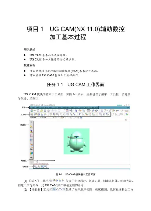
任务1.1 UG CAM工作界面UG CAM模块的基本工作界面，如图1-1所示，主要包含了菜单、工具栏、资源条、导航器、绘图区。

图1-1 UG CAM模块基本工作界面(1) 【插入】工具栏包含了创建程序、创建刀具、创建几何体、创建方法、创建工序等命令，是UG CAM操作中最基础的命令。

(2) 【导航器】工具栏包括了程序顺序视图、机床视图、几何视图和加工方数控加工软件应用(UG NX)法视图命令。

该工具栏通常与【工序导航器】按钮配合使用。

单击【程序顺序视图】按钮，再单击【工序导航器】按钮，该视图用于显示每个工序所属的程序组和每个工序在机床上的执行顺序，如图1-2所示。

图1-2 程序视图下的【工序导航器】窗格单击【导航器】工具栏中的【机床视图】按钮，再单击【工序导航器】按钮，该视图用于显示数控加工中所使用的各种刀具，如图1-3所示。

图1-3 机床视图下的【工序导航器】窗格单击【几何视图】按钮，再单击【工序导航器】按钮，该视图用于显示加工中所存在的几何体和坐标系，以及隶属于几何体下的加工工序，如图1-4所示。

图1-4 几何视图下的【工序导航器】窗格项目1 UG CAM(NX 11.0)辅助数控加工基本过程任务1.2 UG CAM(NX 11.0)基本加工流程UG CAM是UG软件的辅助制造模块，可以实现对复杂零件的自动编程数控加工，主要具备数控车、数控铣、数控钻、线切割等加工功能。

UG CAM和UG CAD紧密集成，UG CAM可以提供全面的、易于使用的功能，以解决数控刀具加工轨迹的生成、加工仿真和加工验证等问题。

本次任务以图1-5所示零件为例，简要说1.2 基本加工流程.mp4 明UG CAM模块的基本加工流程和操作方法。

CTTREE树型控件使用帮助CTTREE是个层次树型控件。

该控件是一种能够以分层格式显示项目的特殊列表框类型。

CTTREE控件典型应用于显示文档标题、索引条目、文件目录结构或其它任何益于分层格式的数据。

CTTREE控件由一系列节点对象组成。

每个节点都可以含有自已的文本（或标签）、位图、检查框与选项按钮。

在列表中的每个节点项都能拥有下级子项。

这些子项以缩进的层级表示。

当一个父项展开时，它的最近的子项变为可见。

当父项收缩时，它的所有子项变为隐藏。

文件名：控件文件: CTTREE.OCX许可文件: ctTree.lic类名：CCtTreeCtrl一.控件的不同部分不同项目的变化用于构建树的节点。

包括：•文本: 每个节点的实际文本。

•+/-图片: 这些图片指示子项是可见还是隐藏。

加号图片指示子项可见，减号图片指示子项隐藏。

•打开/关闭/树叶图片: 这些图片也能指示子项是可见还是隐藏。

树叶图片指示节点无子项。

•图形图像: 每个节点可以包含一个独立的位图。

•树线: 用于链接父项和子项的垂直与水平线。

二.添加控件节点有五种方法用于添加一个节点至控件，它们是：AddNode, AddFontNode, AddPictureNode, AddPictureFontNode与InsertNode方法。

前四个方法间的不同之处是方法所接收的参数不同。

然而，对每个方法来说前三个参数是共有的，它们是：•1 –文本: 将放置于节点的文本•2 –插入类型: 指定节点如何插入•3 –级次: 指定节点要放置的级次插入类型：有三种不同的插入类型。

这些类型的有效值包括：0 –插入一个新的节点至控件尾。

1 –插入一个新的节点至当前选定节点之前2 –插入一个新的节点至当前选定节点之后如果你使用1或2的值来插入节点, 在插入节点之后, 新增的节点将成为选定节点。

0 值不会引起原有选定节点值发生改变。

这么做的目的是更易于插入节点序列而不用经常重定位你所选属性。

关于numpy 使用手册：NumPy（Numerical Python的简称）是Python语言的一个扩展程序库，支持大量的维度数组与矩阵运算，此外也针对数组运算提供大量的数学函数库。

对于Python 程序员来说，NumPy 是进行科学计算的核心库，提供了简单易用的数组对象和丰富的函数来处理多维数组对象。

以下是一些使用NumPy 的建议和要点：1. 安装与导入：首先，您需要安装NumPy 库。

可以使用pip（Python 的包管理器）来安装。

在命令行中输入以下命令即可完成安装：`pip install numpy`。

安装完成后，您可以在Python 脚本或交互式会话中导入NumPy 并使用其功能：`import numpy as np`。

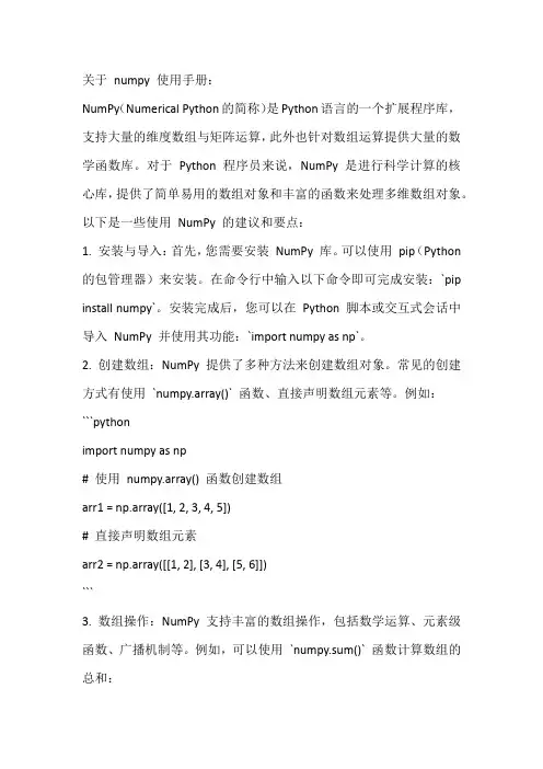
2. 创建数组：NumPy 提供了多种方法来创建数组对象。

常见的创建方式有使用`numpy.array()` 函数、直接声明数组元素等。

例如：```pythonimport numpy as np# 使用numpy.array() 函数创建数组arr1 = np.array([1, 2, 3, 4, 5])# 直接声明数组元素arr2 = np.array([[1, 2], [3, 4], [5, 6]])```3. 数组操作：NumPy 支持丰富的数组操作，包括数学运算、元素级函数、广播机制等。

例如，可以使用`numpy.sum()` 函数计算数组的总和：```pythonimport numpy as nparr = np.array([1, 2, 3, 4, 5])total = np.sum(arr) # 输出结果为15```4. 多维数组：NumPy 支持多维数组对象，这对于处理复杂的数据结构非常有用。

例如，二维数组可以用于表示矩阵运算：```pythonimport numpy as np# 创建一个3x3 的二维数组（矩阵）arr_2d = np.array([[1, 2, 3], [4, 5, 6], [7, 8, 9]])```5. 函数库：NumPy 提供了大量的数学函数来处理数组对象。

NXOpenC++程序员帮助文档006NXOPEN C +++ 10.0简明教程Project，并编译、执行、调试该程序。

第二章应用程序的界面设计第一节MenuScript MenuScript 是用户修改，增加和创建新的用户菜单的工具，用它可以对标准的UG_GATEWAY_MAIN_MENUBAR和UG_GATEWAY_VIEW_POPUP菜单进行修改和编辑。

下面是一些常用的语句。

CREATE ：创建一个新的菜单EDIT ：编辑一个菜单BUTTON ：按钮CASCADE BUTTON：下拉式按钮SEPERATION ：分隔符TOGGLE BUTTON：复选按钮BEFORE 和AFTER：指明菜单的位置MODIFY ：修改一个菜单ACTIONS它可以跟以下内内容STANDARD----它指向标准的UG应用User-Defined Callback----它指向用户定义的回调函数UIStyler dialog ---- 它指向一个UIStyler 对话框GRIP Program File ----- 它指向一具GRIP 程序EXAMPLE1: VERSION 120 EDIT UG_GATEWAY_MAIN_MENUBAR BEFORE UG_HELP CASCADE_BUTTON LAUNCH_CASCADE LABEL Dialog Launcher END_OF_BEFORE MENU LAUNCH_CASCADE BUTTON DEMO_BTN LABEL Display demo dialog ACTIONS demo END_OF_MENU MENUSCRIPT_FILE_ID PVFKENPPAC EXAMPLE2: VERSION 120 EDITUG_GATEWAY_MAIN_MENUBAR MODIFY APPLICATION_BUTTON UG_APP_MODELING LIBRARIES ufx_menuscript_ufsta.sl MENU_FILES/APPEND ufx_menuscript_modeling.menEND_OF_MODIFY MENUSCRIPT_FILE_ID PPDMERMPAG 第二节UIstyler 1. UIstyler对话框设计工具有关对话框设计工具的使用请参考用户手册。

NUKE_5.0和6.0中英对照翻译NUKE 5 节点中英文对照lmage(图像）lmage英文菜单中文翻译Read 读取Write输出Constant常量CheckerBoard棋盘格Draw（绘制）Draw英文菜单中文翻译Bezier贝塞尔曲线Dither抖色DustBust重塑Grain晶粒ScannedGrain扫描晶粒Glint闪光Grid网格Flare耀斑Lightwrap光线包裹Time(时间）Time英文菜单中文翻译Add 3:2pulldown添加3:2下拉Remove3:2pulldown移除3:2下拉AppendClip添加素材FrameBlend帧融合FrameHold帧保持FrameRange帧范围oFlow0流Shannel(通道）Shannel英文菜单中文翻译Shuffle调动ShuffleCopy调动复制Copy复制lmage英文菜单中文翻译ColorBars彩条ColorWheel色轮CurveTool曲线工具Viewer视图Draw英文菜单中文翻译MarkerRemoval标志移除Paint画笔Noise噪波Radial放射Ramp渐变Rectangle矩形Sparkles闪光Text文本Time英文菜单中文翻译Retime重设时间TemporalMedian时间中间点TimeBlur时间模糊NotimeBlur无时间模糊TimeEcho时间延迟timeOffset时间偏移TimeWarp时间扭曲Channel英文菜单中文翻译ChannelMerge通道合并Add添加Remove去除Color(色彩）Color英文菜单中文翻译Match匹配Add加Multiply乘i Gamma伽马ClipTest素材测试ColorMatrix色彩矩阵Expression表达式3D LUT三维LUTCMSTestPattern CMS测试模式GenerateLUT创建LUTVectorfield矢量场Clamp压制ColorLookup色彩查找Colorspace色彩空间ColorTransfer色彩变化Colorcorrect色彩校正Crosstalk色度亮度干扰Filter(滤镜）Filter英文菜单中文翻译Blur模糊Bilateral双面`BumpBoss凹凸Convolve卷积Defocus散焦DegrainBlue去除蓝色DegrainSimple单一去除DirBlur方向模糊EdgeBlur边缘模糊EdgeDetect边缘检测Emboss浮雕Erode(fast)快速侵蚀Erode(filter)过滤侵蚀Erode(blur)模糊侵蚀Color英文菜单中文翻译Exposure 曝光Grade等级Histogram直方图HistEQ平整直方图HueCorrect色相校正HueShift色相转移HSVTool HSV工具Invert反转Log2Lin Log和Lin转换MinColor Min色彩Posterize多色调分色显示RolloffContrast滚边差别Saturation饱和度Sampler采样SoftClip软素材Truelight真实光照Filter英文菜单中文翻译Glow发光GodRays上帝之光Laplacian拉普拉斯算子LevelSet级别设置Matrix矩阵Median重心MotionBlur2D二维运动模糊MOtionBlur3D三维运动模糊Sharpen锐化Soften柔化VectorBlur矢量模糊VolumeRays体积光Zblur深度模糊Zslice深度剪切Keyer(抠像）keyer英文菜单中文翻译Difference差异抠像HueKeyer色调抠像IBKGizmo IBKGizmo抠像IBKColour IBK色彩Keyer抠像器Primatte Primatte抠像Merge(合并）Merge英文菜单中文翻译Addmix添加混合Keymix抠像混合ContactSheet联络表CopyBBox复制界限盒CopyRectangle复制矩形Dissolve叠化LayerContactSheet层联络表Merge合并Merges合并Plus加Matte遮片Multiply乘In里Out外Screen屏幕Max最大Min最小Absminus差异MergeExpression合并表达式Switch切换TimeDissolve时间叠化Premult预乘Unpremult解除预乘Blend 融合Zmerge深度合并Transform(变换）Transform英文菜单中文翻译Transform变换TransformMasked 变换遮罩Card3D三维卡片AdjustBBox调整界限盒BlackOutside黑边CameraShake摄像机颤动Crop剪切CornerPin角钉SphericalTransform球形化变换Idistort I扭曲LensDistrotion镜头畸变Mirror镜像Position位置Reformat重设格式Reconcile3D调整三维PointsTo3D点到三维Tracker跟踪TVlscale TVI缩放GridWarp网格变形SplineWarp样条线变形Stabilize稳定STMap ST映射。

FINE/Turbo V9.1-1新功能郭然NUMECA China目录§1. IGG/AutoGrid (4)§1.1.Flexlm based security ID updated to v14 (4)§1.2.General upgrades in package (4)§1.3.Introduce clustering around control lines (5)§1.4.Parasolid Library v19.1Introduce clustering relaxation for partial gap (6)§1.5.Define partial gap by penny rotation cylinder (7)§1.6.Introduce blade-to-blade full multigrid smoother (8)§1.7.Introduce ZR meridional effect rotating parts definition (9)§1.8.Identify blade pressure & suction sides (11)§1.9.Enforce cell width at blade wall (12)§1.10.Improvements in CEDRE export (13)§1.11.Introduce meridional and blade-to-blade mesh export (14)§1.12.Added python commands (15)§2. FINE/Turbo (16)§unch Harmo2Time in CFView (16)§2.2.Unlimited access to FINE GUI (16)§2.3.Improved Suspend/Kill buttons (16)§e NUMECA logo instead of Tk icon (17)§2.5.Improved automatic block/patch qrouping of zr effects (17)§2.6.Improved management of fluid properties (18)§2.7.Ability to output Static Energy (18)§2.8.Ability to use Non reflecting 2D RS with condensable fluids (18)§2.9.Ability to use CPU Booster with condensable fluids (19)§2.10.Ability to use Laplacian smoothing with rotation periodic BC (19)§2.11.Improved interpolation method of 2D profile (19)§2.12.Introduce generalized transition model with EARSM (20)§2.13.Advanced control for NLH computations (20)§2.14.Introduced NLH frequency crossing terms (21)§2.15.Increased number of boundary nodes for RBF (21)§2.16.Added forced motion with modal coupling (22)§2.17.Ability to run modal coupling with NLH (22)§2.18.Improved finebatch (23)§2.19.Improved finebatch Ability to run NLH with SST turbulence model (23)§2.20.Improved finebatch Ability to use k-epsilon Yang-Shih, SST and EARSM turbulence models with CPU Booster (23)§3. CFView (24)§3.1.Ability to post process in parallel (24)§3.2.Ability to match ranges (24)§3.3.Ability to compute Lambda 2 and Q Invariant quantities (24)§3.4.Ability to compute Isentropic Mach Number (25)§3.5.Ability to compute derived quantities using thermodynamic tables (26)§3.6.Improvements for Harmo2Time (27)§3.7.Ability to launch Harmo2Time in batch (28)§3.8.Ability to compare two computations (29)§3.9.Ability to compute volume integral of a quantity (29)§3.10.Added shortcuts (30)§3.11.Ability to compute meridional average for unstructured projects (30)§3.12.Ability to import unstructured meshes (31)§3.13.Free light CFView version (32)§4. AutoBlade (33)§4.1.New throat-based model for axial blades (33)§4.2.Extend support for target channel curves in geomTurbo format (34)§4.3.Introduce solid model of the blade (34)§4.4.Ability to use multiple geometry analysis windows (35)§4.5.Ability to compute surface curvature (36)§4.6.Ability to compute draft angle for casting process (36)§4.7.Automatic curve attraction for the distance tool (37)§4.8.Apply a scaling to multiple parameters (37)§4.9.Ability to quickly switch between single/multiple view mode (38)§4.10.Ability to build solid body (38)§4.11.Extended range of MLE and MTE (39)§5. Design3D (40)§5.1.Specific license keys for Design3D jobs (40)§5.2.Ability to manage multi-stage database generation / optimization (40)§5.3.Ability to restart a database generation computation (41)§5.4.Enhanced management of invalid samples for ANN (41)§5.5.Ability to restart a database generation computation (41)§5.6.Improved managements of external CFD package mode (42)§5.7.Ability to perform multidisciplinary optimization (43)§5.8.Ability to perform multi-objective optimization (44)§1.IGG/AutoGrid§1.1. Flexlm based security ID updated to v14FINE™/Turbo requiresFlexLM based license keys forexecution. In FINE™/Turbo v9.1, the security ID hasbeen upgraded from v11(starting v9.0)to v14, thusrequiring the delivery of new license keys forexecution.Customer BenefitsNoneKnown LimitationsNone§1.2. General upgrades in packageStarting FINE™/Turbo v9.1,general upgrades are madein package:∙use ofParasolid™ v26.0.∙use of CATIA V5R23Customer BenefitsSupport up to Parasolid™v26.0 and CATIA V5 23.§1.3. Introduce clustering around control linesThe clustering can be relaxedalong a control line by auserdefined factor (RelaxationFactor in the controlline Properties menu) on hub,shroud or mid-span (RelaxationLocation in the controlline Properties menu).Customer BenefitsAvoid clustering wall in channel(along control lines) whenmatching connection betweenchannel and zr effect.Known LimitationsThe option is not available forinlet/outlet of a row, control linesinvolved in bulb, in nozzle and in afan on fin definition.§1.4. Introduce clustering relaxation for partial gapIn configuration with partial gap,the ClusteringRelaxation parameter in the PartialGap Properties dialog box controls therelaxation of the partial gap streamwiseclustering on layers not involved in thepartial gap definition.Customer BenefitsAvoid clustering on layers notinvolved in the partial gap definition.Known LimitationsThe cell width expansion may lead tobad mesh quality if there is not enoughspace on blade to expand the partial gapcell width with the given expansionfactor. Reasonable expansion factor withrespect to the geometry shouldtherefore be defined.§1.5. Define partial gap by penny rotation cylinderThe streamwise bounds (% from leading/trailing edge) of the partial gap can be defined by a cylinder through a diameter, origin and axis. In the whole gap the location of the cylinder will be respected to define the local % from leading/trailing edge on each layer.Customer BenefitsMore controls to define partial gap geometry.Known Limitations∙Solid part of the gap won’t be cylindrical.∙If the option is deactivated, then the partial gap is notrespecting the cylinderdefinition and is generatedusing the classical algorithm: thesame chord length percentagesfor all layers.∙The partial chord lengths in the graphic are updated each time acylinder parameter is modified.In some cases, this may takesome time since the flow pathshave to be generated for thisoperation.§1.6. Introduce blade-to-blade full multigrid smootherhe full multigrid smoother (Full Multigrid OptimizationSteps in Optimization Properties dialog box) allows to accelerate theblade-to-blade smoothingby performing optimization steps on all coarse grids to optimize each coarser grid before performing optimization steps on finest grid level (Optimization Steps on Fine Grid) with orwithout Multigrid Acceleration.As full multigrid smoother produces already a quite good mesh, therefore a reduced number of iteration steps on fine grid is needed after.Customer BenefitsThe full multigrid smoother allows to accelerate the blade-to-blade smoothing process especially when dealing with fine mesh or mesh requesting high amount of iteration steps on fine grid to reach a good mesh quality (initial mesh far from final mesh, e.g. configuration with large skin block).Known Limitations∙This option is notrecommended for coarsemeshes having few multigridlevels for which fine gridsmoothing is already quite fast.∙The full multigrid smoother is not applied in gaps andif Skewness Control is setto Medium or Full.∙The full multigrid smootheras the fine grid smoothermay lead to angulardeviation problems if themesh is includingnon-matching and/ornon-matching periodicconnections.∙The full multigrid smootheris not recommended whendealing with roundedleading/trailing edge bladeand H&I topology withoutskin block.§1.7. Introduce ZR meridional effect rotating parts definitionTheblock and patch in the ZRmeridional effects can be set as rotating:∙the block rotation speed in the ZR effect derivesautomatically from the rowto which the ZR effect isconnected. This informationis propagated to connectedblocks till a rotor/stator isencountered.∙the boundary (patch)rotation speed in the ZReffect is imposedunder Properties in the ZReffect edit mode (QuickAccess Pad) and is applied ifthe patch belongs to arotating geometry. Thegeometry curve isconsidered as rotating ifcreated as Solid PolylineRotating in the ZR effectedit mode or if importedand definedas rotating basic curve. Customer BenefitsAutomate block and patch settings of the ZR meridional effects.Known Limitations∙ A basic curve name cannot contain the keyword"rotating" if its propertiesare set to non rotating,because correspondingpatch name will finallycontain the keyword"rotating".∙Block rotation speed iscomputed automatically butare not interfaced per block.Therefore if some blocks of aZR effect are modified after3D generation (blocksplitting, transformation,...)the rotation speed may belost.∙If the mesh is loaded inIGG™. and resaved, it willstill be correct becauseblock rotation speed comesfrom the configuration whichhas been reread. However ifthe mesh is loaded inAutoGrid5™ and resaved,block rotation speed stillcomes fromconfiguration but which isrecomputed, and thereforeblock rotation speed will benull.§1.8. Identify blade pressure & suction sidesThe Swap Blade PatchesName option is introducedas a 3D mesh control toallow the user to swap thepressure side and thesuction side definition (usedin the patch names) of eachrow to respect the physics.In addition a newpreference Family NameControl/Bladepressure/suctionsides is availablefor CEDRE/CGNS export tosplit the blade family nameinto a pressure side "_PS"and a suction side "_SS"family names.Customer BenefitsControl on thepressure/suction side torespect the physics.Known LimitationsStarting AutoGrid5™v9.1-1, to respect sameconvention for all types ofconfiguration, thepressure/suction sides willbe reversed for double bluntconfiguration.§1.9. Enforce cell width at blade wallStarting AutoGrid5™ v9.1, the option Enforce Cell Width at Blade Wall in 3D Mesh Control dialog box is by default active to minimize the difference between the imposed cell width and the measured one.Customer BenefitsCell width specified by the users at the blade wall can be ensured. Known Limitations∙This development is available for O4H (default) and H&Itopologies only.∙The 3D post-process assumes that the cell width variescontinuously around theblade. Therefore, if there arediscontinuities in the cellwidth of the blade, thepost-process tends to producekinks.∙The 3D post-process is notapplied in gap blocks and thusmay lead to an increase of theinter-block expansion ratiobetween skin block and gapblocks.∙When Cell Width at WallInterpolation option isactivated in theblade-to-blade mesh controls,this post-treatment will bedeactivated automatically.§1.10. I mprovements in CEDRE exportWhen exporting mesh in CEDRE format (File/Export/CEDRE), new options are available in a new dialog box:∙block group(s), block list, all blocks or blocks perrow (if AutoGrid5™) canbe exported.∙all selected blocks can be exported in a singleunstructured block(BlocksMerging option).∙In case of merging, theuser is able to select thename of the merged block(by default setto “DOMAIN_1”). Customer BenefitsMore controls when performing CEDRE export. Known Limitations∙Non matching connection type is not allowed forexport because CEDREdoes not support suchconnection.∙If the block selectioncontains CON or PERpatches and theconnected block is notcontained in the list, theexport cannot beperformed.∙When exporting Rowby Row, only rowmeshes are saved andnot the zr effectmeshes. A zr effect meshcan be only exportedwhen using other blockselection options.§1.11. I ntroduce meridional and blade-to-blade mesh exportAfter selecting the rows, the meridionaland blade-to-blade mesh (on the activelayer (Active Layer (% span))) can beexported in CGNS respectively withthe File/Export/MeridionalMesh and B2B Mesh menu. Theexported CGNS file will only contain theblock points coordinates of the mesh.Customer BenefitsAbility to export meridional andblade-to-blade mesh in CGNSformat.Known Limitations∙The blade-to-blade mesh doesnot include 3D mesh controls asnon-axi treatment, hub/shroudinterpolation, etc.∙When exporting blade-to-blademesh, the spanwise layer iscomputed for each rowaccording to the spanpercentage, whereas in theblade-to-blade view inAutoGrid5™. It is onlycomputed based on the first rowselected, then the closest flowpath is chosen for the otherrows. The method used whenexporting blade-to-blade meshallows in bypass case to obtainthe desired layer on whateverrow.§1.12. A dded python commandsExisting python commands are adapted while new ones are introduced.Customer BenefitsMore python commands available for§2.FINE/Turbo§2.1. Launch Harmo2Time in CFViewThe executable Harmo2Time hasbeen integratedinto CFView™.When the user selects themenu Modules/Harmo2Time, theHarmo2Time in CFView™ will becalled to reconstruct the currentNLH computation in time/space.Customer BenefitsReconstruct NLH computationsin CFView§2.2. Unlimited access to FINE GUIThe user is now able to open an unlimitednumber of FINE GUI.Customer BenefitsSet up projects at the same time.§2.3. Improved Suspend/Kill buttonsThe menu Solver/Suspend isrenamed as Solver/Save andStop. The buttons Save andStop/Kill are also updated.Customer BenefitsClearer indication.§2.4. Use NUMECA logo instead of Tk iconThe Tk icon on the graphic user interface isreplaced by the NUMECA logo.Customer BenefitsBetter GUI view.§2.5. Improved automatic block/patch qrouping of zr effectsThe automatic grouping of the zr effects is improved based on the settings in the AutoGrid5 meshes:∙In the BoundaryConditions page under thetab SOLID, the rotation speed ofall the solid patches of the ZReffects will be set based on therotation speed of the ZR effects,which is defined in theturbomachinery section of the .bcsfile with thekeyword BOUNDARIES_ROTATION_SPEED. The patch grouping willalso depend on the rotation speed.∙In the Rotating Machinery page, the block grouping of the zr effectswill depend on the rotation speed.∙In the Fluid Structure pageunder the tab Thermal, ifapplicable, there will be twogroups for zr effects (fluid/solid).§2.6. Improved management of fluid propertiesStartingfrom FINE™/Turbov9.1, the fluid properties willbe defined only in thefluid section insidethe .iec file. Both theGUI and the flow solverwill use the fluidproperties in thissection.§2.7. Ability to output Static EnergyStarting fromFINE™/Turbo v9.1, the usercan output the static energyfor the computations usingcondensable fluid.Customer BenefitsAccurately compute derivedquantities in CFView.§2.8. Ability to use Non reflecting 2D RS with condensable fluidsStartingusertheinterface and condensable fluids.Customer BenefitsUse Non reflecting RS withcondensable fluids.§2.9. Ability to use CPU Booster with condensable fluidsStartingthecombiningcondensable fluids.Customer BenefitsSave CPU time forcomputations with condensablefluids.§2.10. A bility to use Laplacian smoothing with rotation periodic BCStarting from FINE™/Turbo v9.1,the user can simulate rigid motionwith rotation periodic boundaryconditions.Customer BenefitsFlexibility to generate thecomputational domains.§2.11. I mproved interpolation method of 2D profileWhen a 2D profile is applied to aboundary condition and the 2Dprofile has a low resolution, theinterpolated distribution at theboundary condition by the linearinterpolation may be bad. A newinterpolation method, barycentricinterpolation, is applied in the flowsolver, in order to generate asmoother distribution. Thenew barycentric interpolation can beactivated by setting the expertparameter BC2DIN to 1.Customer BenefitsHigher accuracy using 2D profile.§2.12. I ntroduce generalized transition model with EARSMFINE™/Turbov9.1-1 extends thegeneralized transition model to supportthe EARSM turbulence model. Inaddition to the existing EARSM modelproposed by Menter, the EARSM modelproposed by Hellsten is also added.Customer BenefitsSimulate transition with the EARSMturbulence model.§2.13. A dvanced control for NLH computationsFINE™/Turbo v9.1-1 introduces severalexpert parameters to improve therobustness of NLH computations in case ofpreconditioning:PPRINI: Initializes the real and imaginaryparts of the harmonic pressure (by default100Pa). It is suggested to set the value to(0,0) for low speed flow computations incase that convergence problem appears orthe solution near the Rotor/Stator interfacesis not normal.HAVMOD: introduce new pressure sensor(value -1). This new pressure sensor shouldbe activated in case of shock waveoscillations or low Mach number flows withstrong unsteady motion.VUNS2: coefficient controlling the unsteadypreconditioning velocity in order to be able torun harmonic method for low speed flowapplications.Customer BenefitsImproved robustness for NLH.§2.14. I ntroduced NLH frequency crossing termsBy default, the transportequations for theunsteadyperturbations are obtained byretaining the first-order terms in the basicunsteady flow equations. Thus the influenceof harmonic crossing is omitted. Theharmonic crossing terms can be included bysetting the expert parameter ICROSH to 1.Note, when using ICROSH=1, the CPU timewill be higher than ICROSH=0.Customer BenefitsImproved accuracy for NLH.Known Limitations∙Limited to perfect gas∙Limited to 1 perturbation∙Not compatible withpreconditioning∙Not compatible with IVELSY = 0∙Not compatible with IDECOU = 1∙Not compatible with FSI§2.15. I ncreased number of boundary nodes for RBFThe limited number of boundary nodes inthe mesh deformation using Radial BasisFunctions (RBF) has been increasedCustomer BenefitsPerform larger simulation with meshdeformation.§2.16. A dded forced motion with modal couplingA forced motionmethod isadded in the modalcoupling module, whichallow the user to impose thedeformation of thestructure through its eigenmodes.Customer BenefitsImpose meshdeformation of thestructure.§2.17. A bility to run modal coupling with NLHThe modal coupling has been extended tosupport the harmonic method. With thiscombination, the user is able to perform aflutter analysis with only one blade channelat a low CPU time. For the moment, only theforced motion is supported. The user needsto define the generalized displacement inthe frequency domain. Then, the simulationwill be run by the harmonic method for boththe flow and the structure.Customer BenefitsReduced CPU time for aeroelasticanalysis .Known Limitations∙Not compatible with ITURRC = 2∙Only compatible with modalforced motion.∙Only compatible with Radial BasisFunctions for mesh deformation∙Restricted to 1 perturbation (theforced vibration)∙.globalforce_harmonic file is notcompatible with IFRCTO = 1/2/3§2.18. I mproved finebatchThe finebatch command is improved, whichallows the user to give the arguments inarbitrary order. Two new arguments -nbintand -nbreal are introduced, allowing theuser to define the required integer and realmemory, respectively.Customer BenefitsFlexibility to run finebatch.§2.19. I mproved finebatch Ability to run NLH with SST turbulence modelThis feature is included in the package but itmay require additional calibration. Thecorresponding Technology Readiness Levelis set to 3 and no explanation is availableyet in the official documentationpackage. Contact NUMECA local sales orsupport office for more information.§2.20. I mproved finebatch Ability to use k-epsilon Yang-Shih, SST and EARSM turbulence models with CPU BoosterThis feature is included in the package but itmay require additional calibration. Thecorresponding Technology Readiness Levelis set to 3 and no explanation is availableyet in the official documentationpackage. Contact NUMECA local sales orsupport office for more information.§3. CFView§3.1. Ability to post process in parallelCFView ™ can be started in parallel byusing two new arguments, i.e. -np and -openmp. These arguments allow the user to perform the post processing with the number of threads specified.Customer BenefitsSpeed up the post processing time.§3.2. Ability to match rangesItis possibleto match the colormap ranges for two projects in CFView ™.Customer BenefitsImproved user-friendliness.§3.3. Ability to compute Lambda 2 and Q Invariant quantitiesIt is possible to compute Lambda 2 and Q invariant quantities that are used for vortex detection for any vector fields in CFView ™.Customer BenefitsAdded possibility to compute Lambda 2 and Q invariant quantities.§3.4. Ability to compute Isentropic Mach NumberIt is possible to compute Isentropic Mach Number quantity for computations with Perfect Gas, Real Gas or Condensable fluid in CFView™.Customer BenefitsAdded possibility to compute Isentropic Mach Number.§3.5. Ability to compute derived quantities using thermodynamic tablesIt is possible to compute thederived quantities usingthermodynamic tables in CFView™as it is done in the FINE™/Turbo solver.Customer BenefitsAdded possibility to computethermodynamic quantities.Known Limitations∙The quantities like Density,Static Energy, Static Enthalpy,Static Pressure, StaticTemperature, relative and/orabsolute velocities andturbulent kinetic energy whenapplicable must be outputtedfrom the solver in order toproperly re-compute thedependent variables andimprove the consistencybetween the derived quantitiesin CFView™ and the computedquantities by the solver.∙It should be noted that thetables dedicated to storecomplex non-linear relationsbetween the variables and thesolver outputs often consists ina simple interpolation at cellvertices from values computedin the cell centers. An exactequality cannot be expectedbetween the derived quantitiesin CFView™ and the onescomputed by the solver. Thedifference can reach more than1% in high gradient zones.§3.6. Improvements for Harmo2TimeSomecapabilities are addedfor CFView™/Harmo2Time:∙possibility to reconstructsolution for harmoniccomputation with FSI.∙creation of additional files during the reconstruction. I.e. plot3dand .mf files.∙reconstruction of solution at the control points defined.∙selection of harmonics used in the reconstruction.Customer BenefitsImprove reconstruction of results with CFView™/Harmo2Time.Known Limitations∙The .mf files are not created ifsome blocks have been deselectedby the user. For rank-2 projects,the .mf files are only created if thesolution is reconstructed in time.∙If a block is unselected in the Partial Loader dialog box, thecontrol points in that block arediscarded. The maximumnumber of control points is 200.∙The harmonic selection forreconstruction is not possiblefor rank-2 projects.∙Only the reconstruction in timeis possible for harmonic computation with FSI.§3.7. Ability to launch Harmo2Time in batchCFView™/Harmo2Time canbelaunched in batch by using the commands below with the two new arguments, i.e. -h2t_gui and -h2t. For examples the commands on LINUX:∙ cfview<version> -h2t_gui project-path/project-name .run -print∙ cfview<version> -h2t project-path/project-name .h2t -printThe -h2t_gui argument opens the Partial Loader dialog box for the user to set and save the options of the reconstruction whereas the -h2t argument allows the reconstruction with the parameters given in the .h2t file. 。

CFD网格的分类，如果按照构成形式分，可以分为结构化和非结构化结构化：只能有六面体一种网格单元，六面体顾名思义，也就是有六个面，但这里要区分一下六面体和长方体。

长方体(也就是所有边都是两两正交的六面体)是最理想完美的六面体网格。

但如果边边不是正交，一般就说网格单元有扭曲(skewed). 但绝大多数情况下，是不可能得到完全没有扭曲的六面体网格的。

一般用skewness来评估网格的质量，sknewness=V/(a*b*c). 这里V是网格的体积，a，b，c是六面体长，宽和斜边。

sknewness越接近1，网格质量就越好。

很明显对于长方体，sknewness=1. 那些扭曲很厉害的网格，sknewness很小。

一般说如果所有网格sknewness>0.1也就可以了。

结构化网格是有分区的。

简单说就是每一个六面体单元是有它的坐标的，这些坐标用,分区号码(B),I,J,K四个数字代表的。

区和区之间有数据交换。

比如一个单元，它的属性是B=1, I=2,J=3,K=4。

其实整个结构化单元的概念就是CFD计算从物理空间到计算空间mapping的概念。

I,J,K可以认为是空间x,y,z在结构化网格结构中的变量。

非机构化：可以是多种形状，四面体（也就三角的形状），六面体，棱形。

对任何网格，都是希望网格单元越规则越好，比如六面体希望是长方形，对于四面体，高质量的四面体网格就是正四面体。

sknewness的概念这里同样适用，sknewness越小，网格形状相比正方形或者正四面体就越扭曲。

越接近1就越好。

很明显非结构化网格也可以是六面体，但非结构化六面体网格没有什么B,IJK的概念，他们就是充满整个空间。

对于复杂形状，结构化网格比较难以生成。

主要是生成时候要建立拓扑，拓扑是个外来词，英语是topology，所以不要试图从字面上来理解它的意思。

其实拓扑就是指一种有点和线组成的结构。

工人建房子，需要先搭房粱，立房柱子，然后再砌砖头。

第1章 DPM的装配过程模拟简介通过本课程的学习，了解DELMIA数字化装配过程模拟。

1．创建DELMIA V5使用环境。

(1)根据将使用的工作台（workbench）选择定制启动（Start-Up）。

(2)学习如何识别，创造新的工具栏（Toolbars）并将其应用在各自的工作台（workbench）上，同时推广到所有可用的命令上。

(3)在所使用的配置中设置选项（Options）。

可以设置通用选项（General Options），标明驱动路径以及所需的特殊数据，核实许可（Licensing）和性能设置（Performance settings）。

设置细节层次（Level of Detail），偏好的可视化（Visualization Preferences）等显示选项（Display Options）。

通过参数（Parameters），定义的产品结构，生成报告（Report Generation），并设置使用单元（the Units）。

2．设定偏好的运作环境，现在将创建必要的工具来生成模拟。

(1)创建一个工具项目录（Project Catalog）和用于组装产品的资源。

此目录将存放资源文档。

在这一点上他们是一些表。

目录还包括了装配产品所必需的工具清单。

(2)编辑目录属性（Catalog Properties）。

i.在目录里运行关键字检索（Keyword Search），以便在目录中大量的清单里找到要查找的项目。

ii.详细说明执行装配的活动（Activities），并定义活动的属性（Attributes）以便进一步定义过程。

iii.然后进行观察，并在一个大的预先存在的目录进行练习，以证明保持目录的好处。

(3)创建一个进程库（Process Library）。

这是一个特殊进程的库。

它是为保存运行特殊进程时的数据记录。

(4)编辑一个过程库属性（Process Library Attribute）。

这些属性提供在库里扩充信息的方法，代表能进一步解释特殊活动特点的任何附加活动信息。

Navicat使用手册1概述Navicat是一个强大的数据库管理和开发工具。

Navicat为专业开发者提供了一套强大的足够尖端的工具，但它对新用户易学、易用。

Navicat使用了极好的图形用户界面(GUI)，可以让你用一种安全和更为容易的方式快速和容易地创建、组织、存取和共享信息。

本文介绍Navicat的常见操作和典型用法，以及对MySQL、SQLServer、Oracle 三种数据库的连接和连接过程中常出现的一些错误问题进行阐述。

2预期读者数通畅联软件新进技术人员数通畅联合作伙伴的技术人员外部IT从业者3使用说明3.1安装说明可参见如下地址下载:#path=%252FMySQL%25E5%258F%258ANavicat解压安装Navicat:本例使用MySQL数据库来进行样例说明，MySQL安装介质以及Navicat客户端下载地址，可参见如下URL: #path=%252FMySQL%25E5%258F%258ANavicat安装过程略，配置向导中字符集设置选择第三项“自定义”，同时将字符集Character Set设置为UTF-8，如下图所示:3.2数据库操作3.2.1连接数据库Connection名称，比如Mysql，localhost 是本机地址，数据库名称添加root，然后建立这个Connection用户名密码是在MySQL安装时指定的。

连接测试:点击’OK’，完成。

在窗口的左侧显示当前所有数据，灰色表示没有打开。

3.2.2创建数据库右击连接名字(localhost)或其他数据库的名字、选择创建数据库在打开的对话框中输入:数据库名、设置字符，确定。

左侧出现新建立的数据库。

3.2.3删除数据库右击数据库，删除数据库3.2.4数据库备份/还原双击打开数据库，找到backups点击 New Backup备份成功以后还原数据库，请点击Restore Backup按钮3.2.5数据库的导出导入导出数据库:打开Navicat ，在我们要到处的数据上面右击鼠标，然后弹出的快捷菜单上点击“Dump SQL File…”，在再次弹出的子菜单项中选择第一个“Structure And data”。

mathmatic使用说明Mathematica教程第1章Mathematica概述 1.运行和启动介绍如何启动Mathematica软件，如何输入并运行命令 2.表达式的输入介绍如何使用表达式3.帮助的使用如何在mathematica中寻求帮助。

第2章Mathematica的基本量 1.数据类型和常量 mathematica中的数据类型和基本常量2.变量变量的定义，变量的替换，变量的清除等3.函数函数的概念，系统函数，自定义函数的方法4.表表的创建，表元素的操作，表的应用5.表达式表达式的操作6.常用符号经常使用的一些符号的意义第3章Mathematica的基本运算 1.多项式运算多项的四则运算，多项式的化简等2.方程求解求解一般方程，条件方程，方程数值解以及方程组的求解3.求积求和求积与求和第4章函数作图 1.二维函数作图一般函数的作图，参数方程的绘图。

2.二维图形元素点，线等图形元素的使用3.图形样式图形的样式，对图形进行设置4.图形的重绘和组合重新显示所绘图形，将多个图形组合在一起。

5.三维图形的绘制三维图形的绘制，三维参数方程的图形，三维图形的设置。

第5章微积分的基本操作 1.函数的极限如何求函数的极限2.导数与微分如何求函数的导数，微分。

3.定积分与不定积分如何求函数的不定积分和定积分，以及数值积分。

4.多变量函数的微分如何求多元函数的偏导数，微分5.多变量函数的积分如何计算重积分6.无穷级数无穷级数的计算，敛散性的判断第6章微分方程的求解 1.微分方程的解微分方程的求解2.微分方程的数值解如何求微分方程的数值解第7章 Mathematica程序设计 1.模块模块的概念和定义方法2.条件结构条件结构的使用和定义方法3.循环结构循环结构的使用第8章 Mathematica中的常用函数 1.运算符和一些特殊常用的和不常用一些运算符号，和系统定义的一些常量及其意义符号，系统常数2.代数运算表达式相关的一些运算函数3.解方程和方程求解有关的一些操作4.微积分相关函数关于求导，积分，泰勒展开等相关的函数5.多项式函数多项式的相关函数6.随机函数能产生随机数的函数函数7.数值函数和数值处理相关的函数，包括一些常用的数值算法 8.表相关函数创建表，表元素的操作，表的操作函数9.绘图函数二维绘图，三维绘图，绘图设置，密度图，图元，着色，图形显示等函数 10.流程控制函数1.1.1Mathematica的启动和运行Mathematica是美国Wolfram研究公司生产的一种数学分析型的软件，以符号计算见长，也具有高精度的数值计算功能和强大的图形功能。

C#（UG）Create and display a dialogPrivate dialog As nxopen.uistyler.Dialogdialog = UI.GetUI().Styler.CreateStylerDialog("Sample.dlg")显示对话框dialog.Show()Alternatively, the UI Styler uses the following instead of the show function you open the dialog from the menu:或者，UI/Styler用以下代码实现从菜单打开的对话框的显示功能。

Dim isTopDialog As BooleanisTopDialog = falsedialog.RegisterWithUIMenu(isTopDialog)How styler items are declared:Private changeDialog As NXOpen.UIStyler.DialogItemPrivate changeStr0 As NXOpen.UIStyler.StringItemPrivate changeReal6 As NXOpen.UIStyler.RealItemHow styler items are initialized:（初始化）changeDialog = theDialog.GetStylerItem("UF_STYLER_DIALOG_INDEX",NXOpen.UIStyler.Dialog.ItemType.DialogItem)changeStr0=theDialog.GetStylerItem("STR_0",NXOpen.UIStyler.Dialog.ItemType.St ringItem)changeReal6=theDialog.GetStylerItem("REAL_6",NXOpen.UIStyler.Dialog.ItemType .RealItem）Register dialog box item callback functionsIn order to register these callbacks, NX provides an API “Add##Handler”, wh ere ## is replaced with “Activate”, “Construct”, “Apply” as shown in following examples. For more information on callbacks of all the dialog items, see the callback section in Dialog Item Reference.When you exit a Styler dialog box normally, the destructor callback is executed at last. Selecting Cancel or OK will invoke Cancel or OK callback first, followed by the destructor callback.Event Handler representation（事件处理程序代表）In case of .NET (VB/C#) APIs, registration is done through Delegates, and represented as:namespace NXOpen.UIStyler{public class StringItem: UIStyler.StylerItem{public delegate int Activate(UIStyler.StylerEvent eventObject);public unsafe voidAddActivateEvent(UIStyler.PushButton.Activate activateevent)();}}In your C# application, the registration will look like this:changeDialog.AddConstructHandler(AddressOf constructor_cb, False)changeDialog.AddOkayHandler(AddressOf ok_cb, False)changeDialog.AddApplyHandler(AddressOf apply_cb, False)changeStr0.AddActivateHandler(AddressOf bend_radius_cb, False)changeReal6.AddActivateHandler(AddressOf tolerance_cb, False)Get and set dialog item attributesThe NX Open API provides get and set methods for the relevant attributes of each dialog item. You can set and get the visibility for a PushButton using the following code. Once you get the dialog item, you can set the property of the item anywhere in your program. Here “thePushButton0” is an object of PushButton dialog item.C#/*Getting visibility attribute*/Boolean isVisible = thePushButton0.Visibility;/*Setting visibility attribute*/thePushButton0.Visibility = true;Launch a dialog from the event callback of another dialogWhile registering a callback, you must determine whether this event can launch another dialog box, depending upon the value of the toggle for “Creates Dialog” on the resource editor. The last argument in every callback registering function indicates this. It is done by setting this argument to “TRUE” or “FALSE”.C#changeAction0 =(NXOpen.UIStyler.PushButton)theDialog.GetStylerItem("ACTION_0",Dialog.ItemType.PushButton);changeAction0.AddActivateHandler(new NXOpen.UIStyler.PushButton.Activate(action_0_act_cb), true);changeAction1 =(NXOpen.UIStyler.PushButton)theDialog.GetStylerItem("ACTION_1",Dialog.ItemType.PushButton);changeAction1.AddActivateHandler(new NXOpen.UIStyler.PushButton.Activate(action_1_act_cb), false);Run a VB application as a journal script1. Choose Tools→Journal→Play. The Journal Manager dialog box opens.2. Click Browse to navigate to the location of the VB file.3. Click Run.Run a VB application using DLL1. Open Microsoft Visual Studio .Net.2. Create a new project:o Choose File→New→Project.o Select Visual Basic Projects, Console Application and type the name with which you want to save the project (for example, test).o Click OK.3. In the Solution Explorer, select the AssemblyInfo.vb file from the project, right-clickand choose Delete from the shortcut menu. A dialog appears warning you that the file will be permanently removed. Click OK.4. In the Solution Explorer, select theModule1.vb file from the project, right-click andchoose Delete from the shortcut menu. A dialog appears warning you that the file will be permanently removed. Click OK.5. Add references for the following files:o NXOpen.dllo NXOpenUI.dllo NXOpen.Utilities.dllo NXOpen.UF.dllIn the Solution Explorer, right-click References under the project. Choose AddReference→Browse→%UGII_ROOT_DIR%\out\managed. Press the CTRL key and select the dlls.6. In the Solution Explorer, highlight the project name, right-click and choose AddExisting Item. Navigate to the location of the .vb file and add it.7. Choose Project Menu→Properties. If you see "Module1" in Startup Projec t, pushdown list, select Startup Project as the new Module name displayed in the list. Click OK.8. Choose Build Menu→Build Solution, or Ctrl + Shift + B, or go to Solution Explorer,select the project name, right-click and select Build. This creates the required dll.9. To run the VB examples, do the following:o Choose File→Execute→NX Open. The Execute User Function dialog box opens.o Navigate to the location of the .dll file. It will be in the <Project Folder>\bin directory under the directory named for the VB project.o Select the .dll file and click OK.SelectionSelection class contains methods that update the selection structure associated with the active dialog box. Some method declarations for class Selection are:namespace NXOpen{class Selectionvoid SetSelectionMask(NXOpen::SelectionHandle * select /** Selection handle */,NXOpen::Selection::SelectionAction action /** Mask action */,const std::vector<NXOpen::Selection::MaskTriple> & mask_array /** Mask triples */);public: void SetSelectionCallbacks(NXOpen::SelectionHandle * select /** Selection handle */,const NXOpen::Selection::FilterCallback& filterproc /** Filter callback for additional user specificfiltering. */,const NXOpen::Selection::SelectionCallback& selcb /** Selection callback for application specificprocessing. */);C#∙To get the selection handleDim selectH As SelectionHandle = changeDialog.GetSelectionHandle()∙Create selection mask array∙Dim selectionMask_array(0) As NXOpen.Selection.MaskTriple∙With selectionMask_array(0)∙.Type = NXOpen.UF.UFConstants.UF_solid_type∙.Subtype = NXOpen.UF.UFConstants.UF_solid_edge_subtype∙.SolidBodySubtype = NXOpen.UF.UFConstants.UF_UI_SEL_FEATURE_ANY_EDGE End With∙Set the selection mask∙UI.GetUI().SelectionManager.SetSelectionMask(selectH,NXOpen.Selection.SelectionAction.ClearAndEnableSpecific, selectionMask_array)∙Set selection procedures∙UI.GetUI().SelectionManager.SetSelectionCallbacks(selectH, AddressOf filter_cb, AddressOf sel_cb)∙Define the filter_cb and sel_cb procedures as follows in order to register this in set selection procedure in the above step.∙Public Function filter_cb(ByVal selectedObject As NXObject, ByVal∙selectionMask_array As NXOpen.Selection.MaskTriple, ByVal∙selectHandle As SelectionHandle)∙As Integer∙ Try∙∙ // write your code here∙∙ Catch ex As NXException∙ ' ---- Enter your exception handling code here -----∙ MsgBox(ex.Message)∙ End Try∙End Function∙∙Public Function sel_cb(ByVal selectedObjects As NXObject(), ByVal ∙deselectedObjects() As NXObject, ByVal selectHandle As∙SelectionHandle)∙As Integer∙ Try∙∙// write your code here∙∙ Catch ex As NXException∙ ' ---- Enter your exception handling code here -----∙ MsgBox(ex.Message)∙ End Try∙ sel_cb = NXOpen.UIStyler.DialogState.ContinueDialog End FunctionDialog box layoutIntroductionAttachment class is used to set the attachment of the dialog item, for example left item, right item, top item, and so on and also the relative positioning of the item (for example, center, left, right, bottom, top). The following sections explain the corresponding NX Open APIs that manipulate the dialog item’s attachment (layout) structure.Set an attachment to dialog ItemFollowing set of APIs are used to set the attachment for a particular dialog box itemC# Attachment attach = changeAction0.InitializeAttachment();attach.SetCenter(false);attach.SetAttachTypeTop(Attachment.AttachType.Dialog);attach.SetTopDialogItem("INT_1");attach.SetTopOffset(0);attach.SetAttachTypeRight(Attachment.AttachType.Dialog);attach.SetRightDialogItem("UF_STYLER_DIALOG_INDEX");attach.SetRightOffset(50);attach.SetAttachTypeLeft(Attachment.AttachType.Dialog);attach.SetLeftDialogItem("UF_STYLER_DIALOG_INDEX");attach.SetLeftOffset(50);changeAction0.SetAttachment(attach);。