
SYM Description of SFT Hamiltonian in a PP-Wave Background
- 格式:pdf
- 大小:206.29 KB
- 文档页数:17

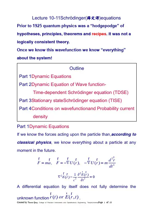
Lecture 10-11Schrödinger(薛定谔)equationsPrior to 1925 quantum physics was a “hodgepodge” of hypotheses, principles, theorems and recipes . It was not a logically consistent theory.Once we know this wavefunction we know “everything” about the system!Part 1Dynamic EquationsIf we know the forces acting upon the particle than,according to classical physics , we know everything about a particle at any moment in the future.22,(),()d r F ma F U r U r m dt ==-∇-∇=r r r r r r r r22221()()0E r E r c t∂∇-=∂r r r r A differential equation by itself does not fully determine theunknown function ()(,)r t or E r t r r r .Part 2Dynamic Equation of Wave function---- Schrödinger equations用21()sin cos 2x kx kx ψ⎡⎤=+⎢⎥⎣⎦描述的粒子,只能有5种动量取值,分别是0,2,2,,k k k k -- ,对应的几率分别是11111,,,,28888,这些几率总和应该为1。
()()1111111()0220,2888811111()128888ki i i k i i p P p p k k k k P p ====⋅+⋅+-⋅+⋅+-⋅==++++=∑∑h h h h 1212(),()1(),()1(),()1k ki i i i i x P x x P x x p x xd x x p x dx x x xd x x d ψψ=======⇒=∑∑⎰⎰⎰⎰¡¡¡¡Do we have the same recipe for calculation of average momentum by using wave function in position representation? Yes, of course, we have!To find the expectation (average) value of p , we first need to represent p in terms of x and t . Consider the derivative of the wave function of a free particle with respect to x:0001(,)exp ()p i x t p x E t ⎡⎤ψ=-⎢⎥⎣⎦h We find that0000000000**000(,)(,)(,)(,)(,)()(,)(,)(,)(0)δ∂ψ=ψ⇒ψ=ψ∂∂==ψ-ψ=ψψ=∂∂-∂⎰⎰p p p p p p p p i x t p x t x t p x t x p p x t i x t dx p x t x t dx i xp x h h h This suggests we define the momentum operator asThe expectation value of the momentum is20022220221()sin cos 2()()()()()=()()()()()ψϕϕϕϕϕ------⎡⎤=+⎢⎥⎣⎦=--++--++k k k k k k k k k k k k x kx kx C x C x C x C x C x x x x x x h h h h h h h h h h h h1()px i p x e ϕ=h ()()111111()022028888===⋅+⋅+-⋅+⋅+-⋅=∑ki i i p P p p k k k k h h h h So,we can not have definite values for the dynamical variables, such as the momentum, when the state of a particle is determined by the wave function with respect to x. We have to find the other way to describe thedynamical variables in Quantum Mechanics.For every dynamical variable or any observable thereis a corresponding Quantum Mechanical OperatorPhysical Quantities →OperatorsOperators are important in quantum mechanics. All observables have corresponding operators.Operators ↔Symbols for mathematical operation✧ The position x is its own operator ˆxx =. Done. Other operators are simpler and just involve multiplication 22x x x x ∧==⋅. ✧ The potential energy operator is just multiplication by V(x).✧ The momentum operator is defined as ˆp i x ∂=-∂h00000002211ˆˆˆˆ1()()[11ˆ(()](())()222ˆ()()())ˆ()()1ˆ()2pp xipp x p xp xix x piix px p pp xix p pp p ppx eipip x i e p eexp x p xx xpT x p p x p p x xpxx eT x T xϕϕϕϕμμμϕϕϕϕϕϕϕμϕ=====⎛⎫∂-=-==⎪∂⎝⎭===hh hhhhh()px xϕ=h000000001(,)exp()1ˆ(,)exp()(,)ˆ(,)(,)pp pp pix t p x E ti iEE x t i p x E t i x ttE x t E x t⎡⎤ψ=-⎢⎥⎣⎦∂⎧⎫⎡⎤⎛⎫ψ=-=ψ-⎬ ⎪⎢⎥∂⎝⎭⎣⎦⎭ψ=ψhh hh h Eigenvalue equation of an operatoreigenvalueDeriving the Schrödinger Equation using operators: This was a plausibility argument, not a derivation. We believe the Schrödinger equation not because of this argument, but because its predictions agree withexperiments.Schrödinger EquationNotes:The Schrödinger Equation is THE fundamental equation of Quantum Mechanics.There are limits to its validity. In this form it applies only to a single, non-relativistic particle (i.e. one withnon-zero rest mass and speed much less than c.)●On the left hand picture 13 velocity vectors of an individual fly are shown; the chain●On the right hand picture the same 13velocity vectors are assigned to 1 fly each todemonstrate that the ensemble average yields the same result, i.e. <v e> = 0,provided that each and every fly does the same thing on average.●i.e. time average = ensemble average. The new subscripts "e" and "r" denote ensemble and space, respectively. This is a simple version of a very far reaching concept in stochastic physics known under the catch word "ergodic hypothesis".●As long as every fly does - on average - the same thing, the vector average overtime of the ensemble is identical to that of an individual fly - if we sum up a fewthousand vectors for one fly, or a few million for lots of flies does not make anydifference. However, we also may obtain this average in a different way:●We do not average one fly in time obtaining <v i>t , but at any given time all flies inspace.●This means, we just add up the velocity vectors of all flies at some moment in timeand obtain <v e>r , the ensemble average. It is evident (but not easy to prove for general cases) thata) Schrödinger equation is a linear homogeneous partialdifferential equation.b) The Schrödinger equation contains the complex number i.Therefore its solutions are essentially complex (unlikeclassical waves, where the use of complex numbers isjust a mathematical convenience.)c) The wave equation has infinite number of solutions,someof which do not correspond to any physical or chemical reality.1. For an electron bound to an atom/molecule, the wavefunction must be everywhere finite, and it must vanish in the boundaries2. Single valued3. Continuous4. Gradient (dψ/dr) must be continuous5. ψψ*dτ is finite, so that ψ can be normalizedd) Solutions that do not satisfy these properties(above)DONOT generally correspond to physicallyrealizable circumstances.e) Conditions on the wave function(波函数的三个基本条件——有限、单值、连续)1. In order to avoid infinite probabilities, the wave functionmust be finite everywhere.2. The wave function must be single valued.3. The wave function must be twice differentiable. Thismeans that it and its derivative must be continuous. (An exception to this rule occurs when V is infinite.)4. In order to normalize a wave function, it must approachzero as x approaches infinity.f) Only the physically measurable quantities must be real.These include the probability, momentum and energy.Can think of the LHS of the Schrödinger equation as a differentialoperator that represents the energy of the particle ?This operator is called the Hamiltonian of the particle , and usually given the symbolˆH.Hamiltonian is a linear differential operator .222ˆ(,)2d V x t H m dx ⎡⎤-+ψ≡ψ⎢⎥⎣⎦h Kineticenergy Potential energyHence there is an alternative (shorthand) form for thetime-dependent Schrödinger equation:Part 3Time-independent Schrödinger equation (TISE), i.e.stationary state(定态)Schrödinger equationSuppose potential is independent of time(),()U x t U x =Look for a separated solution, substitute (,)()()x t x T t ψψ=into• This only tells us that T(t) depends on the energy E . It doesn’t tell us what the energy actually is. For that we have to solve the space part.• T(t) does not depend explicitly on the potential U(x). But there is an implicit dependencebecause the potential affectsthe possible values for the energy E .This is the time-independent Schrödinger equation (TISE) or so-called stationary state Schrödinger equation.Solution to full TDSE isEven though the potential is independent of time the wavefunction still oscillates in time . But probability distribution is static()()2*//2*,,()()()()()iEt iEt P x t x t x e x e x x x ψψψψψ+-=ψ===h hFor this reason a solution of the TISE is known as a StationaryState(定态)Stationary state Schrödinger Equation Notes:• In one-dimension space, the TISE is an ordinary differential equation (not a partial differential equation)• The TISE is an eigenvalue equation for the Hamiltonianoperator:ˆ()()Hx E x ψψ=Part 4 Probability current density and continuity equation Definition of probability current densityIn non-relativistic quantum mechanics, the probability current of the wave function Ψ is defined asin the position basis and satisfies the quantum mechanical continuity equationwith the probability density defined as.If one were to integrate both sides of the continuity equation with respect to volume, so thatthen the divergence theorem implies the continuity equation is equivalent to the integral equationwhere the V is any volume and S is the boundary of V. This is the conservation law for probability in quantum mechanics.In particular, if is a wavefunction describing a single particle, theintegral in the first term of the preceding equation (without the time derivative) is the probability of obtaining a value within V when the position of the particle is measured. The second term is then the rate at which probability is flowing out of the volume V. Altogether the equation states that the time derivative of the change of the probability of the particle being measured in V is equal to the rate at which probability flows into V. Derivation of continuity equationThe continuity equation is derived from the definition of probability current and the basic principles of quantum mechanics. Suppose is the wavefunction for a single particle in the positionbasis (i.e. is a function of x, y, and z). Thenis the probability that a measurement of the particle's position will yield a value within V. The time derivative of this iswhere the last equality follows from the product rule and the fact that the shape of V is presumed to be independent of time (i.e. the time derivative can be moved through the integral). In order to simplify this further, consider the time dependent Schrödinger equationand use it to solve for the time derivative of :When substituted back into the preceding equation for this gives.Now from the product rule for the divergence operatorand since the first and third terms cancel:If we now recall the expression for P and note that the argumentof the divergence operator is justthis becomeswhich is the integral form of the continuity equation .The differential form follows from the fact that the preceding equation holds for all V, and as the integrand is a continuousfunction of space, it must vanish everywhere:For all whole space we have()()2lim lim 0lim lim 0V V V V V S V S dV j dV t j dV j ds →∞→∞→→∞→∞⎛⎫∂ψ ⎪=-∇⋅= ⎪∂⎝⎭∇⋅=⋅=⎰⎰⎰⎰⎰⎰⎰⎰⎰⎰⎰r r r r rwhich meansthat must be continuousat any positionin the whole space.So the wavefunction and its derivative must be continuous.(An exception to this rule occurs when V is infinite.)One more, if the(,)()Et i x t x e ϕ-ψ=hand ()x ϕis real, the probability current*Im ()()0j x x m ϕϕ⎡⎤=∇≡⎣⎦r r h over the whole 1D space which means j r is always continuous whatever the wavefunction ()x ϕand its derivative ()x ϕ'are continuous or not. However, ()x ϕhas to be continuous for an acceptable physical solution for that the probability density is uniquely defined(唯一确定). As to ()x ϕ', it may not be continuous especially at the point where the potential energy is infinite.It is easy to prove that ()x ϕ' has to be continuous at the point 0x where the potential energy just has a limited high step.Have a fun!。


AXIONSGEORG RAFFELTMax-Planck-Institut für Physik(Werner-Heisenberg-Institut),Föhringer Ring6,80805München,Germany(e-mail:*****************.de)(Received7August2001;accepted29August2001)Abstract.Axions are one of the few particle-physics candidates for dark matter which are well motivated independently of their possible cosmological role.A brief review is given of the theoreticalmotivation for axions,their possible role in cosmology,the existing astrophysical limits,and thestatus of experimental searches.1.IntroductionDespite its uncanny success,the particle-physics standard model has many looseends,among them the CP problem of quantum chromodynamics(QCD).The non-trivialfield structure of the QCD ground state(‘ -vacuum’)and a phase of thequark mass matrix each induce a non-perturbative CP-violating term in the QCDLagrangian which is proportional to the coefficient = QCD+arg det M quark, where could lie anywhere between0and2π.The experimental upper limit to aputative neutron electric dipole moment,a CP-violating quantity,informs us that 10−9,a severefine-tuning problem given that is a sum of two unrelated terms which would be expected to be of order unity each.One particularly elegant solution was proposed by Peccei and Quinn,where theparameter is re-interpreted as a dynamical variable, →a(x)/f a,where a(x)isthe axionfield and f a an energy scale called the Peccei-Quinn scale or axion decayconstant(Peccei and Quinn,1977a,b;Weinberg,1977;Wilczek,1977).The previ-ous CP-violating term automatically includes a potential for the axionfield whichdrives it to its CP-conserving minimum(dynamical symmetry restoration).Whilethis may sound complicated,Sikivie(1996)has constructed a beautiful mechanicalanalogy which nicely explains the main features of axion physics.While axions would be very weakly interacting,they are still a QCD phenom-enon.They share their quantum numbers with neutral pions;all generic axionproperties are roughly determined by those ofπ0,scaled with fπ/f a where fπ= 93MeV is the pion decay constant.For example,the axion mass is roughly given by m a f a=mπfπ,and the coupling to photons or nucleons is roughly suppressed by fπ/f a relative to the pion couplings.Axions have not been found during the quarter century since they werefirstproposed,but the interest in this hypothesis is well alive because other proposed Space Science Reviews100:153–158,2002.©2002Kluwer Academic Publishers.Printed in the Netherlands.154G.RAFFELTsolutions of the strong CP problem are not clearly superior,and mainly because axions are one of the few well-motivated particle candidates for the cold dark matter which apparently dominates the dynamics of the universe.The current status of axions physics and astrophysics was reviewed at a recent conference(Sikivie,1999).Particle-physics aspects,the status of astrophysical limits,and that of current search experiments are summarized in three separate mini-reviews in the Review of Particle Physics(Groom et al.,2000).Chapters on axions are also found in some textbooks(Kolb and Turner,1990;Raffelt,1996).For theoretical reviews see Kim(1987)and Cheng(1988),for a review of experimental searches see Rosenberg and van Bibber(2000).2.Stellar-Evolution LimitsThe main argument which proves that the Peccei-Quinn scale f a must be very large, corresponding to a very small axion mass m a,is related to stellar evolution.Axions would be produced by various processes in the hot and dense interior of stars and would thus carry away energy directly,much in analogy to the standard thermal neutrino losses.The strength of the axion interaction with photons,electrons,and nucleons can be constrained from the requirement that stellar-evolution time scales are not modified beyond observational limits(Raffelt,1996).For example,the helium-burning lifetime of horizontal-branch stars inferred from number counts in globular clusters reveals that the Primakoff processγ+Ze→Ze+a must not be too efficient in these stars,leading to a limit of m a 0.4eV(Figure1).Very restrictive limits arise from the observed neutrino signal of the supernova (SN)1987A.After collapse,the SN core is so hot and dense that neutrinos are trapped and escape only by diffusion so that it takes several seconds to cool a roughly solar-mass object the size of a few ten kilometers.The emission of axions would remove energy from the deep inner core which should show up in late-time neutrinos.Therefore,the observed duration of the SN1987A neutrino signal provides the most restrictive limits on the axion-nucleon coupling(Figure1).In the early papers on this topic,the difficulty of calculating the axion emission from a dense and hot nuclear medium had been underestimated;the most recent discussions attempt an inclusion of dense-medium effects(Janka et al.,1996).If axions are too‘strongly’interacting,they are trapped in a SN core,inval-idating the energy-loss argument and implying a mass above which axions are not excluded by the SN1987A signal(Turner,1988;Burrows et al.,1990).They would still carry away some of the energy and would cause excess counts in the water Cherenkov detectors which registered the neutrinos,allowing one to exclude another interval of axion masses(Engel et al.,1990).Probably there is a small crack of allowed axion masses between these two SN1987A arguments(Figure1), sometimes called the‘hadronic axion window’.Therefore,infine-tuned axion models where the tree-level coupling to photons nearly vanishes,eV-mass axionsAXIONS155Figure1.Astrophysical and cosmological exclusion regions(hatched)for the axion mass m a or the Peccei–Quinn scale f a.An‘open end’of an exclusion bar means that it represents a rough estimate. The globular cluster limit depends on the axion-photon coupling;it was assumed that E/N=83as in GUT models or the DFSZ model.The SN1987A limits depend on the axion-nucleon couplings; the shown case corresponds to the KSVZ model and approximately to the DFSZ model.The dot-ted‘inclusion regions’indicate where axions could plausibly be the cosmic dark matter.Most of the allowed range in the inflation scenario requiresfine-tuned initial conditions.Also shown is the projected sensitivity range of the search experiments for galactic dark-matter axions.may be allowed and could thus play the role of a cosmological hot dark matter component(Moroi and Murayama,1998).The axion coupling to electrons can be constrained from the properties of glob-ular-cluster stars and the white-dwarf luminosity function.However,the tree-level existence of such a coupling is not generic,and the resulting limits on m a and f a do not extend the range covered by the previous arguments.3.CosmologyIn the early universe,axions come into thermal equilibrium only if f a 108GeV, a region excluded by the stellar-evolution limits.For f a 108GeV cosmic axions are produced nonthermally.If inflation occurred after the Peccei-Quinn symmetry breaking or if T reheat<f a,the‘misalignment mechanism’(Preskill et al.,1983; Abbott and Sikivie,1983;Dine and Fischler,1983;Turner,1986)leads to a contri-bution to the cosmic critical density of a h2≈1.9×3±1(1µeV/m a)1.175 2i F( i)156G.RAFFELTwhere h is the Hubble constant in units of100km s−1Mpc−1.The stated range re-flects recognized uncertainties of the cosmic conditions at the QCD phase transition and of the temperature-dependent axion mass.The function F( )with F(0)=1 and F(π)=∞accounts for anharmonic corrections to the axion potential.Be-cause the initial misalignment angle i can be very small or very close toπ,there is no real prediction for the mass of dark-matter axions even though one wouldexpect 2i F( i)∼1to avoidfine-tuning the initial conditions.A possiblefine-tuning of i is limited by inflation-induced quantumfluctu-ations which in turn lead to temperaturefluctuations of the cosmic microwave background(Lyth,1990;Turner and Wilczek,1991;Linde,1991).In a broad class of inflationary models one thusfinds an upper limit to m a where axions could be the dark matter.According to the most recent discussion(Shellard and Battye,1998) it is about10−3eV(Figure1).If inflation did not occur at all or if it occurred before the Peccei-Quinn symme-try breaking with T reheat>f a,cosmic axion strings form by the Kibble mechanism (Davis,1986).Their motion is damped primarily by axion emission rather than gravitational waves.After axions acquire a mass at the QCD phase transition they quickly become nonrelativistic and thus form a cold dark matter component.The axion density is similar to that from the misalignment mechanism,but in detail the calculations are difficult and somewhat controversial between one group of authors(Davis,1986;Davis and Shellard,1989;Battye and Shellard,1994a,b)and another(Harari and Sikivie,1987;Hagmann and Sikivie,1991;Hagmann et al., 2001).Taking into account the uncertainty in various cosmological parameters one arrives at a plausible range for dark-matter axions as indicated in Figure1.4.Experimental SearchIf axions are indeed the dark matter of our galaxy one can search for them by the ‘haloscope’method(Sikivie,1983).The generic two-photon vertex which axions posess in analogy to neutral pions allows for the Primakoff conversion a↔γin the presence of external electromagneticfields.Therefore,the galactic axions should excite a microwave resonator which is placed in a strong magneticfield, i.e.,one expects a narrow line above the thermal noise of the cavity.While this line would not be difficult to identify once it has been found,searching for it requires to step a tunable cavity through many resonance intervals in order to cover a given m a range.In the late1980s,this method was pioneered in two pilot experiments (Wuensch et al.,1989;Hagmann et al.,1990).At the present time two full-scale ‘second generation’axion haloscopes are in operation,one in Livermore,Califor-nia(Hagmann et al.,1998,2000)and one in Kyoto,Japan(Ogawa et al.,1996; Yamamoto et al.,2001),the latter one using a beam of Rydberg atoms as a low-noise microwave detector.The projected sensitivity shown in Figure1covers the lower end of the plausible mass range for dark-matter axions.If axions are indeedAXIONS157 the galactic dark matter,these experiments for thefirst time are in a position to actually detect them.Axions or axion-like particles are currently also searched by the‘helioscope’method(Sikivie,1983;van Bibber et al.,1989).Axions would be produced in the Sun by the Primakoff effect,and could be back-converted into X-rays in a long dipole magnet oriented toward the Sun.A dedicated experiment of this sort in Tokyo has recently reported new limits(Inoue et al.,2000)while a much larger ef-fort using a decommissioned LHC test magnet,the CAST experiment,is currently under construction at CERN(Zioutas et al.,1999).It should be noted,however, that these searches are unrelated to axion dark matter,i.e.,if axions were to show up at CAST they almost certainly could not provide the cosmic dark matter.The evidence for the reality of dark matter has mounted for several decades,and most recently culminated with the determination of the cosmological parameters by cosmic-microwave precision experiments and other arguments.On the other hand, the physical nature of dark matter remains as mysterious as it was two decades ago. Therefore,the direct search experiments for particle candidates such as axions are among the most important efforts in the area of experimental cosmology.AcknowledgementsThis research was supported,in part,by the Deutsche Forschungsgemeinschaft under grant No.SFB-375and by the ESF network Neutrino Astrophysics.ReferencesAbbott,L.and Sikivie,P.:1983,‘A Cosmological Bound on the Invisible Axion’.Phys.Lett.B120, 133–136.Battye,R.A.and Shellard,E.P.S.:1994a,‘Global String Radiation’.Nucl.Phys.B423,260–304. Battye,R.A.and Shellard,E.P.S.:1994b,‘Axion String Constraints’.Phys.Rev.Lett.73,2954–2957;(E)ibid.76,2203–2204(1996).Burrows,A.,Ressel,T.and Turner,M.:1990,‘Axions and SN1987A:Axion trapping’.Phys.Rev.D42,3297–3309.Cheng,H.-Y.:1988,‘The Strong CP Problem Revisited’.Phys.Rept.158,1–89.Davis,R.L.:1986,‘Cosmic Axions from Cosmic Strings’.Phys.Lett.B180,225–230.Davis,R.L.and Shellard,E.P.S.:1989,‘Do Axions Need Inflation?’.Nucl.Phys.B324,167–186. Dine,M.and Fischler,W.:1983,‘The Not So Harmless Axion’.Phys.Lett.B120,137–141. Engel,J.,Seckel,D.and Hayes,A.C.:1990,‘Emission and Detectability of Hadronic Axions from SN1987A’.Phys.Rev.Lett.65,960–963.Groom,D.E.et al.:2000,‘The Review of Particle Physics’.Eur.Phys.J.C15,1–878.See also /Hagmann,C.and Sikivie,P.:1991,‘Computer Simulation of the Motion and Decay of Global Strings’.Nucl.Phys.B363,247–280.Hagmann,C.,Chang,S.and Sikivie,P.:2001,‘Axion Radiation from Strings’.Phys.Rev.D63, 125018(12pp).158G.RAFFELTHagmann,C.et al.:1990,‘Results from a Search for Cosmic Axions’.Phys.Rev.D42,1297–1300. Hagmann,C.et al.:1998,‘Results from a High-Sensitivity Search for Cosmic Axions’.Phys.Rev.Lett.80,2043–2046.Hagmann,C.et al.:2000,‘Cryogenic Cavity Detector for a Large-Scale Cold Dark-Matter Axion Search’.Nucl.Instrum.Meth.A444,569–583.Harari,D.and Sikivie,P.:1987,‘On the Evolution of Global Strings in the Early Universe’.Phys.Lett.B195,361–365.Inoue,Y.et al.:2000,‘Recent Results from the Tokyo Axion Helioscope Experiment’.astro-ph/0012338.Janka,H.-T.,Keil,W.,Raffelt,G.and Seckel,D.:1996,‘Nucleon Spin Fluctuations and the Supernova Emission of Neutrinos and Axions’.Phys.Rev.Lett.76,2621–2624.Kim,J.E.:1987.‘Light Pseudoscalars,Particle Physics and Cosmology’.Phys.Rept.150,1–177. Kolb,E.W.and Turner,M.S.:1990,‘The Early Universe’.Addison-Wesley,Reading,Mass. Linde,A.:1991,‘Axions in Inflationary Cosmology’.Phys.Lett.B259,38–47.Lyth,D.H.:1990,‘A Limit on the Inflationary Energy Density from Axion Isocurvature Fluctua-tions’.Phys.Lett.B236,408–410.Moroi,M.and Murayama,H.:1998,‘Axionic Hot Dark Matter in the Hadronic Axion Window’.Phys.Lett.B440,69–76.Ogawa,I.,Matsuki,S.and Yamamoto,K.:1996,‘Interactions of Cosmic Axions with Rydberg Atoms in Resonant Cavities Via the Primakoff Process’.Phys.Rev.D53,R1740–R1744. Peccei,R.D.and Quinn,H.R.:1977a,‘CP Conservation in the Presence of Instantons’.Phys.Rev.Lett.38,1440–1443.Peccei,R.D.and Quinn,H.R.:1977b,‘Constraints Imposed by CP Conservation in the Presence of Instantons’.Phys.Rev.D16,1791–1797.Preskill,J.,Wise,M.and Wilczek,F.:1983,‘Cosmology of the Invisible Axion’.Phys.Lett.B120, 127–132.Raffelt,G.G.:1996,‘Stars as Laboratories for Fundamental Physics’.University of Chicago Press. Rosenberg,L.and van Bibber,K.:2000,‘Searches for Invisible Axions’.Phys.Rept.325,1–39. Sikivie,P.:1983,‘Experimental Tests of the“Invisible”Axion’.Phys.Rev.Lett.51,1415–1417;(E) ibid.52,695(1984).Sikivie,P.:1996,‘The Pool Table Analogy to Axion Physics’.Physics Today49,22–27. Sikivie,P.(ed.):1999,‘Proceedings Axion Workshop’.Nucl.Phys.B(Proc.Suppl.)72,1–238. Shellard,E.P.S.and Battye,R.A.:1998,‘Cosmic Axions’.astro-ph/9802216.Turner,M.S.:1986,‘Cosmic and Local Mass Density of“Invisible”Axions’.Phys.Rev.D33,889–896.Turner,M.S.:1988,‘Axions from SN1987A’.Phys.Rev.Lett.60,1797–1800.Turner,M.S.and Wilczek,F.:1991,‘Inflationary Axion Cosmology’.Phys.Rev.Lett.66,5–8.van Bibber,K.et al.:1989,‘Design for a Practical Laboratory Detector for Solar Axions’.Phys.Rev.D39,2089–2099.Weinberg,S.:1978,‘A New Light Boson?’.Phys.Rev.Lett.40,223–226.Wilczek,F.:1978,‘Problem of Strong P and T Invariance in the Presence of Instantons’.Phys.Rev.Lett.40,279–282.Wuensch,W.U.et al.:1989,‘Results of a Laboratory Search for Cosmic Axions and Other Weakly Coupled Light Particles’.Phys.Rev.D40,3153–3167.Yamamoto,K.et al.:2001,‘The Rydberg Atom Cavity Axion Search’.hep-ph/0101200. Zioutas,K.et al.:1999,‘A Decommissioned LHC Model Magnet as an Axion Telescope’.Nucl.Instrum.Meth.A425,482–489.See also http://axnd02.cern.ch/CAST/。
