T-test

你要检验两独立样本均数差异是否能推论至总体，而行的t检验两样本(如某班男生和女生)某变量(如身高)的均数并不相同，但这差别是否能推论至总体，代表总体的情况也是存在著差异呢？会不会总体中男女生根本没有差别，只不过是你那麼巧抽到这2样本的数值不同？为此，我们进行t检定，算出一个t检定值。

与统计学家建立的以「总体中没差别」作基础的随机变量t分布进行比较，看看在多少%的机会(亦即显著性sig值)下会得到目前的结果。

若显著性sig值很少，比如<0.05(少於5%机率)，亦即是说，「如果」总体「真的」没有差别，那麼就只有在机会很少(5%)、很罕有的情况下，才会出现目前这样本的情况。

虽然还是有5%机会出错(1-0.05=5%)，但我们还是可以「比较有信心」的说：目前样本中这情况(男女生出现差异的情况)不是巧合，是具统计学意义的，「总体中男女生不存差异」的虚无假设应予拒绝，简言之，总体应该存在著差异。

每一种统计方法的检定的内容都不相同，同样是t-检定，可能是上述的检定总体中是否存在差异，也同能是检定总体中的单一值是否等於0或者等於某一个数值。

至於F-检定，方差分析(或译变异数分析，Analysis of Variance)，它的原理大致也是上面说的，但它是透过检视变量的方差而进行的。

它主要用于：均数差别的显著性检验、分离各有关因素并估计其对总变异的作用、分析因素间的交互作用、方差齐性(Equality of Variances)检验等情况。

4，T检验和F检验的关系t检验过程，是对两样本均数(mean)差别的显著性进行检验。

惟t检验须知道两个总体的方差(Variances)是否相等；t检验值的计算会因方差是否相等而有所不同。

也就是说，t检验须视乎方差齐性(Equality of Variances)结果。

所以，SPSS在进行t-test for Equality of Means的同时，也要做Levene's Test for Equality of Variances 。

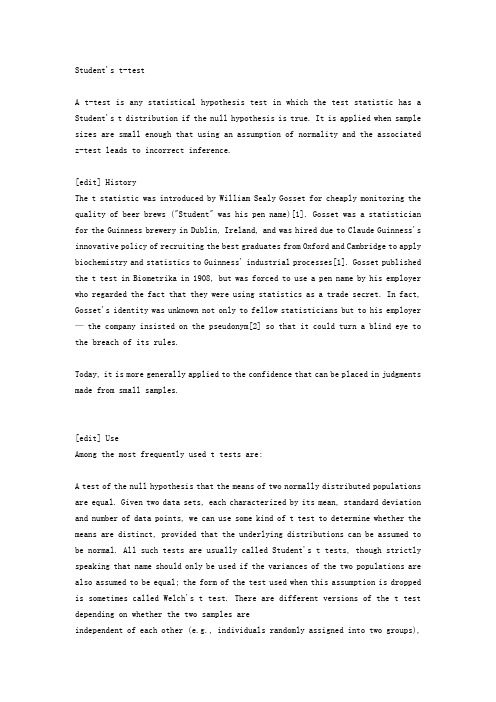
Student's t-testA t-test is any statistical hypothesis test in which the test statistic has a Student's t distribution if the null hypothesis is true. It is applied when sample sizes are small enough that using an assumption of normality and the associated z-test leads to incorrect inference.[edit] HistoryThe t statistic was introduced by William Sealy Gosset for cheaply monitoring the quality of beer brews ("Student" was his pen name)[1]. Gosset was a statistician for the Guinness brewery in Dublin, Ireland, and was hired due to Claude Guinness's innovative policy of recruiting the best graduates from Oxford and Cambridge to apply biochemistry and statistics to Guinness' industrial processes[1]. Gosset published the t test in Biometrika in 1908, but was forced to use a pen name by his employer who regarded the fact that they were using statistics as a trade secret. In fact, Gosset's identity was unknown not only to fellow statisticians but to his employer — the company insisted on the pseudonym[2] so that it could turn a blind eye to the breach of its rules.Today, it is more generally applied to the confidence that can be placed in judgments made from small samples.[edit] UseAmong the most frequently used t tests are:A test of the null hypothesis that the means of two normally distributed populations are equal. Given two data sets, each characterized by its mean, standard deviation and number of data points, we can use some kind of t test to determine whether the means are distinct, provided that the underlying distributions can be assumed to be normal. All such tests are usually called Student's t tests, though strictly speaking that name should only be used if the variances of the two populations are also assumed to be equal; the form of the test used when this assumption is dropped is sometimes called Welch's t test. There are different versions of the t test depending on whether the two samples areindependent of each other (e.g., individuals randomly assigned into two groups),orpaired, so that each member of one sample has a unique relationship with a particular member of the other sample (e.g., the same people measured before and after an intervention, or IQ test scores of a husband and wife).If the calculated p-value is below the threshold chosen for statistical significance (usually the 0.05 level), then the null hypothesis which usually states that the two groups do not differ is rejected in favor of an alternative hypothesis, which typically states that the groups do differ.A test of whether the mean of a normally distributed population has a value specified in a null hypothesis.A test of whether the slope of a regression line differs significantly from 0. Once a t value is determined, a P value can be found using a table of values from Student's t-distribution.[edit] AssumptionsNormal distribution of data, tested by using a normality test, such as Shapiro-Wilk and Kolmogorov-Smirnov test.Equality of variances, tested by using either the F test, the more robust Levene's test, Bartlett's test, or the Brown-Forsythe test, or the O'Brien test Samples may be independent or dependent, depending on the hypothesis and the type of samples:Independent samples are usually two randomly selected groupsDependent samples are either two groups matched on some variable (for example, age) or are the same people being tested twice (called repeated measures)Since all calculations are done subject to the null hypothesis, it may be very difficult to come up with a reasonable null hypothesis that accounts for equal means in the presence of unequal variances. In the usual case, the null hypothesis is that the different treatments have no effect —this makes unequal variances untenable. In this case, one should forgo the ease of using this variant afforded by the statistical packages. See also Behrens-Fisher problem.[edit] Determining typeFor novices, the most difficult issue is often whether the samples are independent or dependent. Independent samples typically consist of two groups with norelationship. Dependent samples typically consist of a matched sample (or a "paired" sample) or one group that has been tested twice (repeated measures).Dependent t-tests are also used for matched-paired samples, where two groups are matched on a particular variable. For example, if we examined the heights of men and women in a relationship, the two groups are matched on relationship status. This would call for a dependent t-test because it is a paired sample (one man paired with one woman). Alternatively, we might recruit 100 men and 100 women, with no relationship between any particular man and any particular woman; in this case we would use an independent samples test.Another example of a matched sample would be to take two groups of students, match each student in one group with a student in the other group based on an achievement test result, then examine how much each student reads. An example pair might be two students that score 90 and 91 or two students that scored 45 and 40 on the same test. The hypothesis would be that students that did well on the test may or may not read more. Alternatively, we might recruit students with low scores and students with high scores in two groups and assess their reading amounts independently.An example of a repeated measures t-test would be if one group were pre- and post-tested. (This example occurs in education quite frequently.) If a teacher wanted to examine the effect of a new set of textbooks on student achievement, (s)he could test the class at the beginning of the year (pretest) and at the end of the year (posttest). A dependent t-test would be used, treating the pretest and posttest as matched variables (matched by student).[edit] Calculations[edit] Independent one-sample t-testThis equation is used to compare one sample mean to a specific value μ0.Where s is the grand standard deviation of the sample. N is the sample size. The degrees of freedom used in this test is N − 1.[edit] Independent two-sample t-test[edit] Equal sample sizesThis equation is only used when the two sample sizes (that is, the n or number of participants of each group) are equal.Where s is the grand standard deviation (or pooled sample standard deviation), 1 = group one, 2 = group two. The denominator is the standard error of the difference between two means. For significance testing, the degrees of freedom for this test is 2n − 2 where n = # of participants in each group.[edit] Unequal sample sizes, equal varianceThis equation is only used when it can be assumed that the two distributions have the same variance. (When this assumption is violated, see below.) The t statistic to test whether the means are different can be calculated as follows:Where s2 is the unbiased estimator of the variance of the two samples, n = number of participants, 1 = group one, 2 = group two. n − 1 is the number of degrees of freedom for either group, and the total sample size minus 2 is the total number of degrees of freedom, which is used in significance testing. Note that in this case, is the pooled variance of the two samples. The degrees of freedom used in significance testing is n1 + n2 − 2.The statistical significance level associated with the t value calculated in this way is the probability that, under the null hypothesis of equal means, the absolute value of t could be that large or larger just by chance—in other words, it's a two-tailed test, testing whether the means are different where either one or the other might be the larger one if they are different (see Press et al, 1999, p. 616).[edit] Unequal sample sizes, unequal varianceThis equation is only used when the two sample sizes are unequal and the varianceis assumed to be different. See also Welch's t test. The t statistic to test whether the means are different can be calculated as follows:Where s2 is the unbiased estimator of the variance of the two samples, n = number of participants, 1 = group one, 2 = group two. Note that in this case, is not a pooled variance. The degree of freedom used in significance testing is as follows:This equation is called the Welch-Satterthwaite equation.This one is also a two-tailed test.[edit] Dependent t-testThis equation is used when the samples are dependent; that is, when there is only one sample that has been tested twice (repeated measures) or when there are two samples that have been matched or "paired".For this equation, the differences between all pairs must be calculated. The pairs are either one person's pretest and posttest scores or one person in a group matched to another person in another group (see table). The average (XD) and standard deviation (sD) of those differences are used in the equation. The constant μ0 is non-zero if you want to test whether the average of the difference is significantly different than μ0. The degree of freedom used is N-1.。

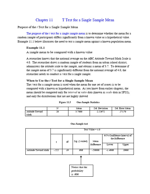
Chapter 11T Test for a Single Sample MeanPurpose of the t Test for a Single Sample MeanThe purpose of the t test for a single sample mean is to determine whether the mean for a random sample of participants differs significantly from a known value or a hypothetical value. Example 11.1 below illustrates the need to test a sample mean against a known population mean.Example 11.1A sample mean to be compared with a known valueA researcher knows that the national average on the ABC Attitude Toward Math Scale is4.0. The researcher draws a random sample of students from an urban school district,administers the attitude scale to the sample, and obtains a mean of 3.7. To determine ifthe sample mean of 3.7 is significantly different from the national average of 4.0, theresearcher needs to conduct a t test for a single sample.When to Use the t Test for a Single Sample MeanThe t test for a sample mean is used when the mean for one set of scores is to becompared with a known or hypothetical mean. As you know from earlier chapters, themean should be computed only for interval or ratio data (known as scale data in SPSS), and only for distributions that are not highly skewedFigure 11.5 One-Sample StatisticsOne-Sample testInterpreting the SPSS OutputIn the output in Figure 11.5, the mean for the sample is 3.7000, and the value of t is -5.25.The probability that the null hypothesis is true is .606 (indicated in SPSS with the term“Sig. [2-tailed]”). Note that by default, SPSS uses a two-tailed tests, which is by far themost frequently used. To interpret the probability value of .606, use the followingguidelines:a.If the probability displayed by SPSS is equal to or less than .001, declare thedifference statistically significant at the .001 level.b.If the probability displayed by SPSS is equal to or less than .01 (but greaterthan .001), declare the difference statistically significant at the .01 level.c.If the probability displayed by SPSS is equal to or less than .05 (but greaterthan .01), declare the differences statistically significant at the .05 leveld.If the probability displayed by SPSS is greater than .05, declare the differencenot statistically significant (i.e. in significant) at the .05 levelBecause .606 (in the output in Figure 11.5) is greater than .05, the differenceis not statistically significant. Because it is not statistically significant, the null hypothesis should not be rejectedChapter 12 Paired-Samples t TestPurpose of the Paired-Samples t TestAs you know, the t test can be used to determine the statistical significance of the difference between two means. In Chapter 11, the procedure for testing the difference between a known mean (such as population mean) and a sample mean was covered.In this chapter, you will learn how to conduct the paired-samples t test. This test is appropriate when each score underlying one mean has been paired (i.e., matched) with a score underlying the other mean. Example 12.1 below illustrated the meaning of paired samples (i.e., with paired scores).Example 12.1An experiment with paired scoresA researcher drew a random sample from a population and administered a depressionscale to the sample. This administration of the scale yielded pre-test scores, for whichthe researcher computed a mean. Then, the researcher administered a new antidepressant drug to the sample. Next, the researcher administered the depression scale again, which yielded posttest scores. As a result, for each pretest score earned by an individual, there is an associated posttest score for the same individual. These sets of scores are pairedscores.To conduct the paired-samples t test, you will be analyzing the scores in table 12.1 below, which are based on example 12.1 above. The researcher wants to determine if the meanof the pretest scores is significantly different from the mean of the posttest scores. Notethat each pretest score is paired with a posttest score (i.e., the pretest score of 10 forParticipant Number 1 is paired with his or her posttest score of 9 by being places in thesame row). To begin, launch SPSS and select “Type in Data,” as described in previouschapters.Table 12.1Pretest and Posttest Depression ScoresParticipant Number Pretest Score Posttest Score1 10 92 12 93 9 104 15 155 11 86 14 107 8 98 13 109 12 7Paired Sample StatisticsPaired Samples CorrelationsInterpreting the SPSS OutputIn the output in Figure 12.7, note that SPSS refers to the probability of .033 as “Sig. 92-tailed).” Because .033 is less than .05 (but greater than .01), the difference between the means is statistically significant at the .05 level. (Refer to the decision rules for interpreting probability levels.) When the difference is statistically significant, the null hypothesis is rejected.Describing the Results of a t test for Paired Samples in a Research Report Reporting the Results of a significant t testFirst, report the mean and standard deviation for each set of scores. Then, report the value of t,and indicate whether it is statistically significant. This is illustrated in Example 12.2 from Figure 12.7 above.Example 12.2“The depression score decreased, from 11.56 (sd=2.30) on the pretest to 9.67(sd=2.24) on the posttest. The difference between the two means is statisticallysignificant at the .05 level (t=2.57, df=8).”As mentioned, it is important to note that SPSS uses the letters “T” and “t.” However, in research reports, you should use lowercase, italicized, t, as it is done above. Also, note that in various places, SPSS hyphenates “T-Test.” In the social and behavioral sciences, this term in not hyphenated. Thus, when discussing the analysis in a research report, it is more important to state “A t test was used…” than to state “A T-Test was used…”Reporting the Results of an Insignificant t TestReport the means and standard deviations for the two sets of scores, followed by the results of the t test. Figure 12.8 below shows the results of an insignificant t test for differences in algebra scores from pretest to posttest. (The scores on which the t test was conducted are not shown in this book. The results of the t test on them are given in order to illustrate how to report the results of an insignificant t test).Note that the probability of .447 is greater than .05, so the difference is not statistically significant. Also, note that the face that the value of t is negative has no bearing on significance; significance is determined solely by the probability (the value of p).Figure 12.8Paired Sample StatisticsPaired Samples Correlationspresented below.Example 12.3Statement that presents the results of an insignificant t test for the output in Figure 12.8. “The average algebra score increased only sl ightly, from 17.11 (sd=3.48) on the pretest to 17.33 (sd=3.87) on the posttest. The difference between the two means is not statistically significant at the .05 level (t=-.800, df=8).”Chapter 13 Independent-Samples t TestPurpose of the Independent-Samples t TestAs you know, the t test can be used to determine the statistical significance of the difference between two means. In Chapter 11, the procedure for testing the difference between a known mean (such as population mean) and a sample mean was covered. In Chapter 12, the use of the t test for paired samples was covered. In this chapter, you will learn how to conduct a t test for two samples that are independent of each other. The term independent indicated that there is no relationship (no matching or pairing) of scores from one sample to the other. Example 13.1 below has independent samples.Example 13.1An experiment with two independent sampleA researcher drew a random sample from a population and showed the sample a film onthe consequences of driving while intoxicated. This sample was the experimental group.For a control group, the researcher independently drew a separate random sample fromthe same population, to which the film was not shown. Then, a questionnaire on attitudes toward drinking and driving was administered, and the mean for each sample wascomputer. Because selection of the individuals for the experimental group had nobearing on the selection of individuals for the control group, the two samples are said to be independent. In other words, they were separately and independently drawn from apopulation.Assigning Numerical Codes to Identify GroupsYou will need to launch SPSS and enter the data from Table 13.1 below, which are based on Example 13.1. Note that there are two variables in the table. The first variable is “Group” (experiemental or control). For analysis by SPSS, you will use the following codes, as shown in the table: 1=experimental group and 2= control group.The second variable is “attitudes toward drinking and driving.” See Examp le 13.1 for a description of the design of the experiment. Note that higher scores indicate a more positive attitude toward drinking and driving.Table 13.1Attitudes Toward Drinking and Driving for Experimental and Control GroupsParticipant Number Group Codes for Groups Attitudes TowardDrinking andDriving1 Experimental 1 122 Control 2 143 Control 2 144 Experimental 1 105 Experimental 1 126 Control 2 157 Experimental 1 88 Control 2 169 Experimental 1 1210 Control 2 1011 Experimental 1 912 Control 2 11Group StatisticsIndependent Samples TestInterpreting and Describing the Results of the Independent-Samples t TestExamine the means in the top box of the output in Figure 13.11 above. The mean of 10.57 for the experimental group indicated that this group has less positive attitudes toward drinking and driving than the control group with a mean of 13.80.Equality of Variances AssumedThe results of two t tests (on the same data) are shown in Figure 13.11 above. In the Second box, the t test in the top row is based on the assumption that the differences in the variances in the two sets of scores are equal. To determine if this is a valid assumption, examine the “Sig.” for “Levene’s Test for Equality of Variances.” (See the arrow in Figure 13.11) The “Sig.” is the probability value for Levene’s Test. If this “Sig.” is greater than .05, it is appropriate to assume equality of variances, and the statistics for the t test in the top row should be used. Because “Sig.” in Figure 13.11 (.795) is greater than .05, the t test in the top row is the appropriate one to use. Thus, the value of t of -2.886 (not -2.715) should be reported, as illustrated in Example 13.2 on the next page.In Figure 13.11, the appropriate value of t is -2.886 and the associated probability (identified in SPSS as “Sig. [2-tailed]” is .016. Because .016 is less than .05 (but greaterthan .01), the difference between the two means is statistically significant at the .05 level. (See the decision rules to review the guidelines for interpreting probability levels.)。

CFA一级的Parametric Test主要涉及到t检验(t-test)、F检验(F-test)以及相关率(correlation coefficient)等统计概念和方法。

以下是一些基本的介绍：
1. t检验：t检验是用来检验两个总体均值是否存在显著差异的一种假设检验方法。

在CFA一级考试中，你需要掌握独立样本t检验（Two Sample t-Test）和配对样本t检验（Paired Sample t-Test）。

2. F检验：F检验也是一种用于比较两组数据均值是否存在显著差异的方法，常用于在多个样本之间进行比较。

3. 相关系数：相关系数是衡量两个变量之间线性关系强度的指标。

在CFA一级考试中，你需要了解皮尔逊相关系数（Pearson Correlation Coefficient）和斯皮尔曼等级相关系数（Spearman Rank Correlation Coefficient）。

以上这些都是CFA一级Parametric Test的核心内容，建议结合实际例子进行理解和记忆，这样能够更好地掌握这些知识点。

t检验t-test临界值表-t检验表第一篇：t检验介绍t检验，又称为Student's t检验，是用于小样本量数据（样本大小少于30）的假设检验方法之一。

t检验可以判断两个样本的均值是否有显著差异。

一般来说，当p值小于0.05时，我们认为两个样本均值存在显著差异，即拒绝原假设；反之，当p值大于等于0.05时，我们认为两个样本均值不存在显著差异，即接受原假设。

t检验有两种，一种是独立样本t检验，另一种是配对样本t检验。

独立样本t检验适用于两个样本之间是独立的情况，比如说男性和女性两组人的身高数据。

而配对样本t检验适用于两个相关样本之间的比较，比如说一个人在某项测试前后的得分。

t检验的基本原理是比较两个样本均值的差异是否显著，其中样本均值的计算方式是样本数据的总和除以样本数量。

而t值的计算方式是样本均值之差除以标准误差的比值，其中标准误差是标准差除以样本数量的平方根。

t值与显著性水平（通常为0.05）一起使用可以得到p值，即两个样本均值是否有显著差异。

需要注意的是，t检验的前提条件是两个样本符合正态分布，如果数据分布不服从正态分布，可能会影响t检验结果的可靠性。

第二篇：独立样本t检验表独立样本t检验表是用于计算t值临界值的表格。

在做独立样本t检验时，需要根据样本大小和显著性水平选择对应的t值临界值。

通常，显著性水平选择0.05，对应的就是95%置信度水平。

下面是样本大小为n1和n2、显著性水平为0.05的独立样本t检验表格：自由度 0.025 0.010 0.005 0.0011 12.706 31.821 63.657 318.3092 4.303 6.965 9.925 22.3273 3.182 4.541 5.841 10.2154 2.776 3.747 4.604 7.1735 2.571 3.365 4.032 5.8936 2.447 3.143 3.707 5.2087 2.365 2.998 3.499 4.7858 2.306 2.896 3.355 4.5019 2.262 2.821 3.250 4.29710 2.228 2.764 3.169 4.14411 2.201 2.718 3.106 4.02512 2.179 2.681 3.055 3.93013 2.160 2.650 3.012 3.85214 2.145 2.624 2.977 3.78715 2.131 2.602 2.947 3.73316 2.120 2.583 2.921 3.68617 2.110 2.567 2.898 3.64618 2.101 2.552 2.878 3.61019 2.093 2.539 2.861 3.57920 2.086 2.528 2.845 3.55221 2.080 2.518 2.831 3.52722 2.074 2.508 2.819 3.50523 2.069 2.500 2.807 3.48524 2.064 2.492 2.797 3.46725 2.060 2.485 2.787 3.45026 2.056 2.479 2.779 3.43527 2.052 2.473 2.771 3.42128 2.048 2.467 2.763 3.40829 2.045 2.462 2.756 3.39630 2.042 2.457 2.750 3.385在使用独立样本t检验时，需要先计算样本均值和标准误差，然后根据样本大小、显著性水平和自由度选择相应的t 值临界值，最后计算t值并比较p值是否小于显著性水平来判断是否拒绝原假设。

独立样本t 检验翻译基本解释●独立样本t 检验：Independent Samples t-test●音标：[ˌɪndɪˈpɛndənt ˈsæmpəlz ˈtiːtɛst]●名词(n) 意思：用于比较两个独立样本的均值是否存在显著差异的统计方法具体用法●名词(n):o用于比较两个独立样本的均值是否存在显著差异的统计方法o同义词：two-sample t-test, unpaired t-test, between-groups t-test, independent t-test, two-group t-testo反义词：paired t-test, dependent t-test, within-subjects t-test, matched-pairs t-test, repeated measures t-testo例句：●The independent samples t-test is commonly used in researchto determine if there is a significant difference between themeans of two groups. (独立样本t 检验常用于研究中，以确定两组均值之间是否存在显著差异。

)●When conducting an independent samples t-test, it isimportant to ensure that the samples are randomly selected and independent of each other. (进行独立样本t 检验时，确保样本是随机选择且相互独立是很重要的。

)●Researchers often use the independent samples t-test tocompare the effectiveness of two different treatments. (研究人员经常使用独立样本t 检验来比较两种不同治疗方法的效果。

利用Excel 计算均值, 标准差, T-TEST 检验教程1. 利用Excel 计算均值1.1 输入数据，将鼠标置将要计算均值的0min列下方，输入=(C4+C5+C6+C7+C8+C9)/6，按回车键即可得到该列数据的均值8.43333。

1.2 将鼠标放在8.43333黑框右下方，变为黑十字形后往D10,E10,F10,G10,H10,I10,J10方向右拉，则可分别得到0min，30min，60min，90min，120min，180min，240min，300min，360min 时血糖均值。

2. 利用Excel 计算标准差2.1 在所需计算方差的列下方键入“=”，在Excel 左上方寻找STDEV,2.2 选中STDEV, 出现“函数参数”对话框，在2.3 点击，选中将要计算的第一组值0min列1,2,3,4,5,6号个体0min时血糖值。

2.4 按回车键，回到“函数参数”对话框，再按“确定”，则在C11出现此列标准差0.898146.将鼠标放在0.898146.黑框右下方，变为黑十字形后往D11,E11,F11,G11,H11,I11,J11方向右拉，则可分别得到0min，30min，60min，90min，120min，180min，240min，300min，360min 时血糖标准差。

同样对腹腔注射hMUP组小鼠0min，30min，60min，90min，120min，180min，240min，300min，360min 时血糖的平均值和标准差。

3. 利用Excel作T-TEST 检验腹腔注射PBS组和腹腔注射hMUP组是否存在差异3.1 在所需计算方差的列下方键入“=”，在Excel 左上方寻找TTEST3.2 选中TTEST, 出现“函数参数”对话框，在3.3 点击，选中将要计算的PBS组值0min列1,2,3,4,5,6号个体0min时血糖值。

3.4 按回车键，回到“函数参数”对话框，在3.5 点击，选中将要计算的hMUP组值0min列11,12,13,14,15,16,17,18,19,20,21号个体0min时血糖值。