Delaunay Triangulation and Voronoi Diagram on the
- 格式:pdf
- 大小:184.76 KB
- 文档页数:19

一种新的求解对流占优问题的自适应网格细化方法郭巍; 张伟伟; 聂玉峰【期刊名称】《《计算力学学报》》【年(卷),期】2019(036)005【总页数】7页(P583-589)【关键词】自适应网格细化; 泡泡型网格生成; SU PG方法; 后验误差估计; 对流占优问题【作者】郭巍; 张伟伟; 聂玉峰【作者单位】西北工业大学理学院西安710129【正文语种】中文【中图分类】O242.11 引言对流扩散方程描述了物质的浓度与温度等的输运过程,方程由扩散项和对流项两部分组成,当对流项占主导作用时,方程的解会出现奇异层,给求解带来困难。
由于奇异层通常很薄,传统的均匀网格很难捕捉到,因此会出现数值震荡的现象。
为了提高数值解的精度,许多学者提出了各种自适应网格细化方法。
自适应网格细化方法在误差大的区域加密网格,在误差小的区域粗化网格,从而用较小的计算量达到满意的精度。
自适应网格细化方法的效果依赖于后验误差估计子和网格细化技术。
针对对流扩散问题的后验误差估计子的研究始于20世纪70年代末,经过多年的发展,目前常用的后验误差估计包括残差型后验误差估计[1]、恢复型后验误差估计[2]和隐式误差估计[3]等。
网格细化技术包括网格重构和网格分割两类。
第一类方法根据后验误差估计重新生成新的网格,其中基于Voronoi 的CVT网格生成方法在自适应有限元计算中已有广泛应用[4,5]。
第二类方法根据单元后验误差估计和标记策略来选取需要加密的单元,然后对标记的单元进行加密操作。
常见的加密操作包括红-绿加密法[6]、二分法[7]和规则加密法[8]等。
这些方法简单易行,然而通常需要网格光顺操作来提高网格质量。
为了生成高质量的网格,Shimda等[9]提出了泡泡布点方法,模拟泡泡在区域中运动直至最后达到力平衡的状态,泡泡的中心组成了最优点集。
同时,针对泡泡布点方法得到的高质量的点集,陈蔚蔚等[10]提出了泡泡型局部网格生成算法(Bubble-type Local Mesh Generation,BLMG),用来高效地生成Delaunay网格。
1. “MATLAB 指令查找”用法说明MATLAB 的功能是通过指令来实现的,要掌握一个软件的使用,就要学会它的指令。
MATLAB 的指令有数千条,对于绝大多数用户而言,要全部掌握这些指令是不可能的,而且也没有必要,因为要用到全部指令的机会几乎为零,本书也不过用到了数百条指令。
但是,有时为了某种特殊用途,需要用到某个特殊指令,这时如何找到这个指令就很重要了。
对此,MATLAB 有一套很完善的指令查找系统,就是按功能查找与按字母顺序查找。
初学者由于不熟悉这套系统的使用方法而很少使用,所以下面对这套指令查找系统作些介绍。
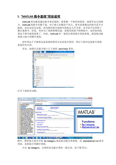
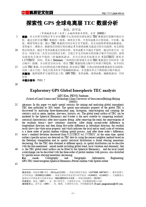
首先,如图点击指令窗口左下角的 start\help 菜单,打开下面的对话框,图中,图形放大部分中的 By Category 就是按功能分类查找,而 Alphabetical List 指令列表,也即按字母顺序查找。
点击 By Category ,出现的是功能分类的一级目录,如下图 所示,再点击任何一条目录,又出现第二级目录,例如点击Mathmatics,出现的是下图,再点击其中的一条目录,又出现第三级目录,如点击Elementary Math,出现的下图,这时又出现第四级目录以及第四级目录下的各种具体的指令,再往下点击就是指令的用法解释。
每级目录都会有简单的说明,而且目录的层次也会在左边的目录系统中体现出来(左边的兰色亮条)。
这时,就可以了解每条指令的具体用法,如下图所示。
至此,查找过程结束。
如果在菜单 Start\help 之后,点击 Alphabetical List 打开的界面是按字母顺序列出的所有指令,点击具体的指令也能找到对应的指令说明。
不过此时,左边的目录系统不会随指令的不同产生相应的改变。
第四 级目录 具体 的指令为了让初学者了解功能分类目录的含义,下面选择性的翻译了部分比较常用内容,以供参考。
2.Function Reference 指令分类总目录2.1. Desktop Tools and Development Environment 桌面工具与运行环境Startup, Command Window, help, editing and debugging, tuning, other general functions 启动,指令窗口,帮助系统,编辑与调试程序,调整,其它一般性功能。

基于机载LiDAR点云和建筑物轮廓线构建DSM的方法李迁;肖春蕾;陈洁;杨达昌【摘要】为了获取高精度的数字表面模型(digital surface model,DSM),提出了利用离散的三维激光点云和建筑物轮廓线构建DSM的方法.首先,利用不规则三角网(triangulated irregular network,TIN)渐进滤波算法对激光点云进行预处理,得到地面点和非地面点;然后,基于高程纹理提取非地面点中的建筑物脚点,根据脚点的深度影像图,利用Canny算子提取建筑物边缘,用方位角聚类规则法对建筑物边缘规则化;最后,采用提取的离散地面点数据和建筑物轮廓矢量线构建DSM.采用柳州地区的一组机载LiDAR数据对该方法进行了实验验证,结果表明,通过该方法构建的DSM,建筑物的边缘信息比较精确.【期刊名称】《国土资源遥感》【年(卷),期】2013(025)002【总页数】6页(P95-100)【关键词】DSM构建;建筑物检测;建筑物边缘提取;边缘规则化【作者】李迁;肖春蕾;陈洁;杨达昌【作者单位】中国国土资源航空物探遥感中心,北京 100083;中国地质大学(北京),北京 100083;中国国土资源航空物探遥感中心,北京 100083;中国国土资源航空物探遥感中心,北京 100083;中国地质大学(北京),北京 100083;中国国土资源航空物探遥感中心,北京 100083【正文语种】中文【中图分类】TP750 引言LiDAR(light detection and ranging,LiDAR)系统包含激光雷达、全球定位系统(GPS)和惯性导航系统(INS)。
激光脉冲不受阴影和太阳角度影响,能够快速、直接且连续自动地获取地面三维数据。
这些数据经过简单的处理(如粗差剔除、格网化),便可以得到一种重要的空间数据——数字表面模型(digital surface model,DSM)。
激光点云为不规则的三维离散点数据,可通过采用逐点内插的方法建立DSM。
Voronoi图的构建和应用侯玉昭(南京航空航天大学机电学院,南京市,210016)摘要:Voronoi图是计算几何中常用而又重要的几何结构,它有很强的实用价值。
本文介绍了平面点集上的Voronoi图的一些生成方法,主要是矢量法和栅格法的原理与生成过程。
其次就是V图在各个领域中的应用和分析了V图的一些优势特点。
以此希望我国科研人员关注V图的研发工作。
关键词:V oronoi图;矢量法;栅格法;V图应用Construction and application of V oronoi diagramHou Yuzhao(College of Aerospace Engineering, Nanjing University of Aeronautics&Astronautics, Nanjing, 210016, China;) Abstract:V oronoi graph is a common and important computational geometry in diagram geometry,it has a strong practical value.This paper introduces some generation method for planar point set on the V oronoi graph,it is mainly the principle and formation process of the vector method and the grid method.The second is the application of V graphs in various fields and analyzes some advantages of V graphs. We hope our researchers focus on R&D of V graph.Key words:V oronoi graph;Vector method;Grid method;Application of V oronoi graph引言Voronoi图的历史是相当古老的。

micromine基本原理与方法4.1 矿床三维模型构建方法运用计算机技术建立矿床三维模型的研究工作从六十年代为解决浸染状矿床建模问题而采用三维块段模型以来,至今已经历了近四十年的发展。
建模方法也由早期简单的方块模型,发展到如今的实体模型。
下面就三维矿床模型建模方法分别进行简要的介绍。
4.1.1 线框模型矿体的地质形态复杂多变,很难用规则的几何体来描述。
它需要一种灵活、简便、快速的方法来建立矿体的不规则几何模型。
目前,比较知名的采矿CAD 系统均是采用表面模型来描述矿体的几何模型。
这种表面模型通常是由一系列的三角面围成的表面。
如MICL的MICROMINE 的线框模型、Maptek 的Vulcan的模型等均是表面模型。
在不同的系统中表面模型的名称不同,但实质都是表面模型。
由于这种表面模型在未渲染前看似由线框构成,因而在采矿CAD系统中多称为线框模型。
不过,这种表面模型可以进行体积估算、表面渲染、切制剖面、快速三维显示等操作,比计算机图形学中的表面模型有所扩展。
能满足矿山设计、生产中地质制图的基本要求,也是建立矿体三维实体模型的基础。
线框模型的构建主要是采用了TIN技术(不规则三角网模型)中的V oronoi 图与Delaunay三角形算法。
TIN是一种表示数字高程模型的方法,它既减少规则网格方法带来的数据冗余,同时在计算效率(如坡度)方面又优于纯粹基于等高线的方法。
TIN模型根据区域有限个点集将区域划分为相连的三角面网络,区域中的任意点落在三角面的顶点、边上或三角形内。
如果点不在顶点上,该点的高程值通常通过线性插值的方法得到(在边上用边的两个顶点的高程,在三角形内则用三个顶点的高程)。
所以TIN是一个三维空间的分段线性模型,在整个区域内连续但不可微。
TIN的数据存储方式不仅要存储每个点的高程,还要存储其平面坐标、节点连接的拓扑关系,三角形及邻接三角形等关系。
TIN模型在概念上类似于多边形网络的矢量拓扑结构,只是TIN模型不需要定义“岛”和“洞”的拓扑关系。
基于Voronoi图的林分空间模型及分布格局研究刘帅;吴舒辞;王红;张江;李建军;王传立【摘要】以南洞庭湖龙虎山次生林为研究对象,建立林分Voronoi图模型,通过该模型表示林分空间结构特征,提取林木空间量化信息.在此基础上,引入变异系数量化Voronoi多边形面积的变化率,将林木空间格局分析转化为计算Voronoi图变异系数,并将计算结果与角尺度作相关性比较.结果表明:林分Voronoi图模型能准确表达林木邻接关系、相邻木距离及角度、空间密度等重要空间信息;大尺度取样时(76m以上),变异系数趋于稳定,林分整体空间格局呈接近随机分布的轻度聚集;Voronoi图变异系数和角尺度存在显著的正相关关系,进一步说明本研究格局分析方法的可行性和有效性;受多种因素影响,乔木层主要树种在不同发育阶段的空间格局表现出强烈的时间和空间动态特性,且小径木多为聚集分布,大径木呈轻度聚集或随机分布.基于Voronoi图的林分空间模型及格局分析方法,从空间上表征林木的生长繁育特性、种内种间关系、资源及环境分布特征,为计算几何方法应用于林分空间经营提供了新的思路.【期刊名称】《生态学报》【年(卷),期】2014(034)006【总页数】8页(P1436-1443)【关键词】Voronoi图;林分空间模型;林分空间格局;角尺度【作者】刘帅;吴舒辞;王红;张江;李建军;王传立【作者单位】中南林业科技大学,长沙410004;中南林业科技大学,长沙410004;中南林业科技大学,长沙410004;湖南省科学技术厅,长沙410013;中南林业科技大学,长沙410004;中南林业科技大学,长沙410004;中南林业科技大学,长沙410004【正文语种】中文与林木空间位置有关的林分结构统称为林分空间结构,主要包含树种混交、大小分化和空间格局3个方面的内容。
林分空间结构决定了林木间的竞争优势及其空间生态位,在很大程度上影响着林分的健康和稳定。
空间数据分析方法空间数据分析方法导语:空间数据分析的方法有什么呢?以下是小编为大家分享的空间数据分析方法,欢迎借鉴!空间数据分析1. 空间分析:(spatial analysis,SA)是基于地理对性的位置和形态特征的空间数据分析技术,其目的在于提取和传输空间信息,是地理信息系统的主要特征,同时也是评价一个地理信息系统功能的主要指标之一,是各类综合性地学分析模型的基础,为人们建立复杂的空间应用模型提供了基本方法.2. 空间分析研究对象:空间目标。
空间目标基本特征:空间位置、分布、形态、空间关系(度量、方位、拓扑)等。
3. 空间分析根本目标:建立有效地空间数据模型来表达地理实体的时空特性,发展面向应用的时空分析模拟方法,以数字化方式动态的、全局的描述的地理实体和地理现象的空间分布关系,从而反映地理实体的内在规律和变化趋势。
GIS空间分析实际是一种对GIS海量地球空间数据的增值操作。
4. ArcGIS9中主要的三种数据组织方式:shapefile,coverage和geodatabase。
Shapefile由存储空间数据的dBase表和存储属性数据和存储空间数据与属性数据关系的.shx文件组成。
Coverage的空间数据存储在INFO表中,目标合并了二进制文件和INFO表,成为Coverage要素类。
5. Geodatabase是面向对象的数据模型,能够表示要素的自然行为和要素之间的关系。
6. GIS空间分析的基本原理与方法:根据空间对象的不同特征可以运用不同的空间分析方法,其核心是根据描述空间对象的空间数据分析其位置、属性、运动变化规律以及周围其他对象的相关制约,相互影响关系。
方法主要有矢量数据的空间分析,栅格数据的空间分析,空间数据的量算与空间内插,三维空间分析,空间统计分析。
7. 栅格数据在数据处理与分析中通常使用线性代数的二维数字矩阵分析法作为数据分析的数学基础。
栅格数据的处理方法有:栅格数据的聚类、聚合分析,复合分析,追踪分析,窗口分析。
第18卷第6期2013年11月气候与环境研究Climatic and Environmental ResearchV ol. 18, No. 6Nov. 2013熊敏诠. 2013. 区域Delaunay三角剖分法在全国平均降水量中的应用[J]. 气候与环境研究, 18 (6): 710–720, doi:10.3878/j.issn.1006-9585.2013.12006. Xiong Minquan. 2013. Research on the application of constrained Delaunay triangulation in precipitation averaged over China [J]. Climatic and Environmental Research (in Chinese), 18 (6): 710–720.区域Delaunay三角剖分法在全国平均降水量中的应用熊敏诠1, 2, 31中国科学院大气物理研究所,北京1000292中国科学院大学,北京1000493国家气象中心,北京100081摘 要介绍了Delaunay三角网的性质及其算法类型;根据1980~2009年全国2200个观测站的降水量资料,将观测点和采集的边界点共同进行普通的Delaunay三角剖分,通过删除边界点及其区域外的三角形以实现区域Delaunay三角剖分,得到了较理想全国陆地的Delaunay三角网;随后对球面上的三角片进行面积计算,在已知站点的经纬度情况下,将大地坐标系转换到空间直角坐标系中,应用平面三角余弦定理获得球面三角内角,从而求得三角片面积,并以面积大小确定各个站点降水量的权重系数,得到全国平均降水量值。
对比分析了30年的全国不同时间尺度(日、月、年)平均降水量,Delaunay三角法对应全国平均降水量均值和标准差都明显低于算术平均法,但是两种方法计算的降水量值的相关系数较高;通过Shapiro-Wilk方法进行正态性检验分析,两种计算方法求得的年平均降水量总体服从正态分布;在方差奇性的F检验中,两者的方差具有非奇性特点;使用t检验,在显著性0.05α=时,Delaunay三角剖分法计算的全国平均降水量总体均值偏小。
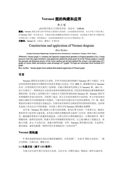
Algorithm772:STRIPACK:Delaunay Triangulation and Voronoi Diagram on the Surface of a SphereROBERT J.RENKAUniversity of North TexasSTRIPACK is a Fortran77software package that employs an incremental algorithm to construct a Delaunay triangulation and,optionally,a Voronoi diagram of a set of points (nodes)on the surface of the unit sphere.The triangulation covers the convex hull of the nodes,which need not be the entire surface,while the Voronoi diagram covers the entire surface.The package provides a wide range of capabilities including an efficient means of updating the triangulation with nodal additions or deletions.For N nodes,the storage requirement for the triangulation is13N integer storage locations in addition to3N nodal ing an off-line algorithm and work space of size3N,the triangulation can be constructed with time complexity O͑N log N͒.Categories and Subject Descriptors:G.1.1[Numerical Analysis]:Interpolation;G.1.2[Nu-merical Analysis]:Approximation;G.4[Mathematics of Computing]:Mathematical Soft-wareGeneral Terms:AlgorithmsAdditional Key Words and Phrases:Delaunay triangulation,Dirichlet tessellation,sphere, Thiessen regions,Voronoi diagram1.INTRODUCTIONThe Delaunay triangulation[Delaunay1934]and its dual,the Voronoi diagram[Voronoi1908],have a large and growing number of applications, among which are finite-element grid generation,scattered data fitting,and the efficient solution of closest-point problems[Preparata and Shamos 1985].Most of the literature on these structures describes the planar case, but the applications also frequently arise in R3and on the surface of a sphere[Augenbaum and Peskin1985;Renka1984a;1997].This material is based upon work supported by the National Science Foundation under Award R-9111671.Author’s address:Department of Computer Sciences,University of North Texas,Denton,TX 76203-1366.Permission to make digital/hard copy of part or all of this work for personal or classroom use is granted without fee provided that the copies are not made or distributed for profit or commercial advantage,the copyright notice,the title of the publication,and its date appear, and notice is given that copying is by permission of the ACM,Inc.To copy otherwise,to republish,to post on servers,or to redistribute to lists,requires prior specific permission and/or a fee.©1997ACM0098-3500/97/0900–0416$5.00ACM Transactions on Mathematical Software,Vol.23,No.3,September1997,Pages416–434.STRIPACK is a revision of the triangulation portion of Algorithm 623[Renka 1984b].The language has been updated to Fortran 77;the data structure has been changed;the time complexity has been reduced;and a number of capabilities have been added.The additions include a subroutine that constructs the Voronoi diagram associated with a given Delaunay triangulation,and a function that locates a point relative to a polygon on the surface of the sphere.These are further discussed in Section 3.Both were motivated by the development of a new model of plate tectonics in which plate motion is driven by the frictional forces exerted by the underlying mantle [Fohlmeister and Renka 1994;Fohlmeister et al.1990].It is assumed that the mantle flow at the surface is directed radially outward from each of a set of hotspots at various locations on the surface of the earth (modeled by the unit sphere).We partition the surface into a set of Voronoi regions (spheres of influence),each centered on a hotspot.Refer to Figure 1.We present definitions in Section 2,some theoretical background in Section 3,a discussion of algorithms in Section 4,and a description of the software package in Section5.Fig.1.Hotspot-centered Voronoi regions (convection cells).Algorithm 772:STRIPACK •417ACM Transactions on Mathematical Software,Vol.23,No.3,September 1997.2.DEFINITIONS AND TERMINOLOGYDenote the unit sphere centered at the origin byUϭ͕pʰR3:ʈpʈϭ1͖,whereʈ⅐ʈis the Euclidean norm on R3.A metric on U is defined by d͑p,q͒ϭarccos͗p,q͘᭙p,qʰU,where͗⅐,⅐͘is the inner product associated with R3,and the angular separation(arclength)between p and q is in the interval͓0,͔.A subset HʚU is convex if,for every pair of points p,qʰH,a geodesic joining p to q(uniquely defined unless d͑p,q͒ϭ)is contained in H.The convex hull H of a finite set S of points of U is the smallest convex set that contains all the points.Note that,if the elements of S are contained in a single hemisphere,H has an interior(the smaller region)and an exterior(the larger region)with a boundary curve consisting of geodesics joining elements of S.Otherwise, H is the entire sphere surface.The convex hull of three distinct points is a (spherical)triangle with the points as vertices.If the vertices are collinear (lie on a common great circle),the triangle is null(has zero area).Let Sϭ͕p i͖iϭ1N denote a set of N distinct elements of U,referred to as nodes,not lying on a common great circle,for NՆ3,and let H denote the convex hull of S.A triangulation T of S is a set of triangles that satisfy the following properties:(1)the triangle vertices are nodes,(2)no triangle contains a node other than its vertices,(3)the triangle interiors are pairwise disjoint,and(4)the union of triangles covers H.It follows from the definition that the set of vertices coincides with S and the triangulation partitions H.If H is contained in a hemisphere,the triangulation has boundary edges(triangle sides that are not shared by two triangles),the endpoints of which are referred to as boundary nodes.An edge that is not a boundary edge is an interior edge,and a node that is not a boundary node is an interior node.A triangle with vertices p i,p j,and p kʰS will be denoted͑p i,p j,p k͒, where the vertices are specified in counterclockwise order,i.e.,det ͑p i,p j,p k͒ϭ͗p iϫp j,p k͘Ն0,where det͑p i,p j,p k͒denotes the determinant of the matrix with rows(columns)p i,p j,and p k in that order, and p iϫp j denotes the vector cross product.The circumcenter of a triangle͑p i,p j,p k͒isv ijkϭ͑p jϪp i͒ϫ͑p kϪp i͒ʈ͑p jϪp i͒ϫ͑p kϪp i͒ʈ.418•Robert J.RenkaACM Transactions on Mathematical Software,Vol.23,No.3,September1997.Algorithm772:STRIPACK•419 Note that since the vertices cannot lie on a common line,v ijk is well defined even for a null triangle.Also,since͗v ijk,p l͘ϭdet͑p i,p j,p k͒/ʈ͑p jϪp i͒ϫ͑p kϪp i͒ʈfor lʰ͕i,j,k͖,v ijk is equidistant from the vertices(as isϪv ijk,but no other point of U).v ijk andϪv ijk are the intersections of the perpendicular bisectors(great circles)of the triangle sides.The circum-radius of͑p i,p j,p k͒is r ijkϭd͑v ijk,p l͒for lʰ͕i,j,k͖,and the circum-circle of͑p i,p j,p k͒isC ijkϭ͕p⑀U:d͑v ijk,p͒ϭr ijk͖.Note that0Ͻr ijkՅ/2,and C ijk contains p i,p j,and p k.A Delaunay triangulation T*of S is a triangulation of S with the empty circumcircle interior property,i.e.,no circumcircle of a triangle of T contains a node in its interior.It is uniquely defined up to the neutral case of four or more nodes lying on a common circle(plane).Delaunay triangu-lations have also been referred to as Thiessen triangulations.The circum-circle property implies a reasonably uniform triangulation which provides a good basis for interpolation of data values associated with the nodes [Lawson1984;Renka1984a;1984b].For each node p iʰS,we define a Voronoi region R i as the closure of the set of points closer to p i than to any other node,i.e.,R iϭ͕pʰU:d͑p,p i͒Յd͑p,p j͒᭙p jʰS͖.The set of Voronoi regions͕R i͖iϭ1N partitions U into a Voronoi diagram,also termed a Dirichlet or Thiessen tessellation[Rhynsburger1973].A Voronoi edge is the intersection of two Voronoi regions that share a point,and a Voronoi vertex is the intersection of three or more Voronoi regions that share a point.Hence Voronoi edges are portions of perpendicular bisectors of geodesics joining pairs of nodes,and Voronoi vertices are circumcenters or negative circumcenters of triangles with vertices in S.3.DUALITY AND EXTENSION OF THE TRIANGULATIONWe now illustrate the duality between the Delaunay triangulation and the Voronoi diagram.This provides the basis for an algorithm that constructs one from the other.The theory for the analogous planar tessellations is well known[Lawson1977;Sibson1978].In that case,there is a one-to-one correspondence between Voronoi regions and triangulation vertices(nodes); Voronoi edges are portions of perpendicular bisectors of triangulation edges;and the set of Voronoi vertices coincides with the set of triangle circumcenters.(In the neutral case of four or more nodes lying on a common circle,one or more Voronoi edges degenerates to a point.)Thus, given a Delaunay triangulation,the Voronoi region associated with a node is defined by the(cyclically)ordered sequence of circumcenters of the triangles containing the node.Conversely,a Delaunay triangulation may be constructed from a Voronoi diagram by connecting nodes whose VoronoiACM Transactions on Mathematical Software,Vol.23,No.3,September1997.420•Robert J.Renkaregions share more than one point and,in the case of k nodes on a common circle for kϾ3,choosing an arbitrary set of kϪ3nonintersecting edges.Both algorithms have operation counts of O͑N͒.We will show that the case of nodes on the surface of the sphere iscompletely analogous to the planar case if the convex hull H is the entire surface.This restriction seems to be an implicit assumption in the litera-ture[Augenbaum and Peskin1985].If the nodes are contained in a single hemisphere,however,the set of Voronoi vertices is a superset of the triangulation circumcenters.The question is then how to select the addi-tional Voronoi vertices in an algorithm for constructing the Voronoi dia-gram from a given Delaunay triangulation.This section is primarily addressed to answering that question.Consider the simplest case in which Nϭ3.There are two Voronoi vertices:the circumcenter and its negative.In the case of four nodes and two triangles,the Voronoi vertices are the two circumcenters along with the negatives of the circumcenters of the other possible pair of triangles (the two triangles obtained by swapping the shared edge for the otherdiagonal).More generally,there are2NϪ4Voronoi vertices,correspond-ing to the number of triangles in a triangulation that covers the surface,while the number of triangles is2NϪN BϪ2for N B boundary nodes if N BϾ0.Thus the number of additional Voronoi vertices is N BϪ2.This is the number of triangles in a triangulation in which all nodes areboundary nodes,and in fact the solution is to construct a triangulation T B of the boundary nodes using an“empty circumcircle exterior”criterion.The additional Voronoi vertices are then the negative circumcenters of the triangles of T B.These may be thought of as the circumcenters of a set of pseudotriangles that cover the exterior of H.The following results make these ideas more precise.L EMMA 3.1.A triangle circumcenter or its negative qϭϮv ijk is a Voronoi vertex if and only if q is not contained in the interior of a Voronoi region,i.e.,for every node p lʰS,d͑q,p l͒Նd͑q,p m͒for some node p m p l.P ROOF.This follows immediately from the definitions.eLet T*be a Delaunay triangulation of S.T HEOREM3.2.If͑p i,p j,p k͒ʰT*,then v ijk is a Voronoi vertex.P ROOF.Suppose͑p i,p j,p k͒ʰT*.Then d͑v ijk,p l͒Նr ijk᭙p lʰS by the empty circumcircle interior criterion.Hence,for every p lʰS,d͑v ijk, p l͒Նd͑v ijk,p m͒for some p m p l(using mʰ͕i,j,k͖Ϫ͕l͖),i.e.,v ijk is a Voronoi vertex by Lemma3.1.eACM Transactions on Mathematical Software,Vol.23,No.3,September1997.Algorithm772:STRIPACK•421 L EMMA3.3.Suppose p i is an interior node of T*.Then,for every triangle ͑p i,p j,p k͒of T*that contains p i,Ϫv ijk is closer to some node p l than to p i,p j,or p k.P ROOF.If some circumcircle C ijk contains all nodes,then every node is a boundary node.Hence,for an interior node p i,C ijk has a node in its exterior,i.e.,᭚p lʰS such that d͑v ijk,p l͒Ͼr ijk,implying that d͑Ϫv ijk,p l͒ϭϪd͑v ijk,p l͒ϽϪr ijkϭd͑Ϫv ijk,p m͒formʰ͕i,j,k͖.eLet p l be the closest node toϪv ijk.Then eitherϪv ijk is not a Voronoi vertex(it is interior to R l)or it is a Voronoi vertex(circumcenter or negative circumcenter)associated with some triangle containing p l.In either case,we have the following.T HEOREM3.4.The negative circumcenterϪv ijk of a triangle of T*that contains an interior node need not be included in the set of Voronoi vertices. (If it is a Voronoi vertex,it coincides with the circumcenter of another triangle or the negative circumcenter of a triangle containing only boundary nodes.)Thus,if all nodes are contained in a single hemisphere,the addi-tional Voronoi vertices(other than v ijk for͑p i,p j,p k͒ʰT*)are negative circumcenters of triangles containing only boundary nodes.By Theorem3.4,the additional Voronoi vertices associated with nodes in a single hemisphere are obtained by triangulating the set of N B boundary nodes S B.Let T B*denote a triangulation of S B in which all triangle circumcircles have no nodes in their exteriors:the complement of a Delau-nay triangulation.T HEOREM 3.5.For each triangle͑p i,p j,p k͒ʰT B*,Ϫv ijk is a Voronoi vertex(in the Voronoi diagram associated with S).P ROOF.For͑p i,p j,p k͒ʰT B*,all nodes of S B are on or interior to C ijk, i.e.,for every node p lʰS B,d͑v ijk,p l͒Յr ijk.Hence d͑Ϫv ijk,p l͒ϭϪd͑v ijk,p l͒ՆϪr ijkϭd͑Ϫv ijk,p m͒᭙mʰ͕i,j,k͖.ThusϪv ijk is not interior to a Voronoi region and is therefore a Voronoi vertex by Lemma3.1.eAs in the case of the Delaunay triangulation,T B*can be constructed from an arbitrary triangulation T B of S B by swapping diagonal arcs in convex quadrilaterals consisting of pairs of adjacent triangles.Note that,in the case of T B*,all such quadrilaterals are necessarily convex.The swap test applied to interior edges is a local application of the circumcircle criterion: the shared edge in a pair of adjacent triangles is swapped out if and only if the fourth vertex is exterior to the circumcircle of(either)one of the triangles.In the case of collinear nodes,T B*will contain null triangles,but their circumcenters are well defined.ACM Transactions on Mathematical Software,Vol.23,No.3,September1997.422•Robert J.RenkaThe following theorem provides a simple computational procedure for applying the swap test without computing distances.The operation count is 9multiplications,14additions,and a comparison.T HEOREM 3.6.Given adjacent triangles͑p i,p j,p k͒and͑p j,p i,p l͒in T B,the diagonals should be swapped if and only ifdet͑p jϪp i,p kϪp i,p lϪp i͒Ͻ0.P ROOF.d͑v ijk,p l͒Ͼr ijkN arccos͗v ijk,p l͘Ͼarccos͗v ijk,p i͘N͗v ijk,p l͘Ͻ͗v ijk,p i͘N͗v ijk,p lϪp i͘ϭͳ͑p jϪp i͒ϫ͑p kϪp i͒,p lϪp iʹϽ0ʈ͑p jϪp i͒ϫ͑p kϪp i͒ʈN det͑p jϪp i,p kϪp i,p lϪp i͒Ͻ0eCorollary3.7.The swap test is well defined,i.e.,given adjacent trian-gles͑p i,p j,p k͒and͑p j,p i,p l͒in T B,p l is exterior to C ijkN p k is exterior to C jilN p i is interior to C kljN p j is interior to C lki.P ROOF.By Theorem 3.6,p l is exterior to C ijk if and only if det͑p jϪp i,p kϪp i,p lϪp i͒ϭdet͑p j,p k,p l͒ϩdet͑p i,p k,p j͒ϩdet͑p i,p j,p l͒ϩdet͑p i,p l,p k͒Ͻ0.Permuting subscripts,p k is exterior to C jil if det͑p iϪp j,p lϪp j,p kϪp j͒ϭdet͑p i,p l,p k͒ϩdet͑p j,p l,p i͒ϩdet͑p j,p i,p k͒ϩdet͑p j,p k,p l͒Ͻ0.Equivalence of the first two criteria follows from equality of the determinants.The other results are obtained by a similar computation:p i is interior to C klj if and only if det͑p lϪp k,p jϪp k,p iϪp k͒Ͻ0,and p j is interior to C lki if and only if det͑p kϪp l,p iϪp l,p jϪp l͒Ͼ0,where det͑p lϪp k,p jϪp k,p iϪp k͒ϭdet͑p kϪp l,p iϪp l,p jϪp l͒ϭϪdet͑p jϪp i,p kϪp i,p lϪp i͒.eACM Transactions on Mathematical Software,Vol.23,No.3,September1997.The following theorem relates the local circumcircle criterion to the global property defining T B *.We define an edge of T B to be locally optimal if and only if it is a boundary edge or it is an interior edge that satisfies the local circumcircle criterion.T HEOREM 3.8.All circumcircles of T B have empty exteriors ͑T B ϭT B *͒if and only if all edges of T B are locally optimal.P ROOF .The “only if”part follows immediately from the definitions.For the other part,suppose the theorem is false,i.e.,that all edges are locally optimal and that there is a circumcircle C ijk with some node p m in its exterior.Refer to Figure 2.We may assume without loss of generality that p k and p m lie on opposite sides of the edge e ij joining p i and p j ,i.e.,e ij is an interior edge,and det ͑p i ,p j ,p m ͒Ͻ0.Among all triangles of T B whose circumcircles have p m as an exterior point,assume without loss of general-ity that none is closer to p m in the sense that they share a point with the geodesic joining p m to an interior point of e ij .Let ͑p i ,p l ,p j ͒be the triangle that shares edge e ij with ͑p i ,p j ,p k ͒.Since e ij is locally optimal,p l is not exterior to C ijk ,and p l p m .If both e il and e lj were boundary edges,then p m would be contained in ͑p i ,p l ,p j ͒.Hence either e il is an interior edge with det ͑p i ,p l ,p m ͒Ͻ0,or e lj is an interior edge with det ͑p l ,p j ,p m ͒Ͻ0.Hence p m is closer to ͑p i ,p l ,p j ͒than ͑p i ,p j ,p k ͒,and a contradiction will be reached if it is shown that p m is exterior to C ilj .The great circle containing p i and p j defines two hemispheres,one of which contains p l ,and the portion of C ilj that lies in this hemisphere is on or interior to C ijk .It follows that p m is exterior to C ilj .eThe following algorithm constructs T B *incrementally.(1)Cyclically order the nodes of S B in counterclockwise order.Denote thesequence by ͕p i ͖i ϭ1N B.Fig.2.Theorem 3.8.Algorithm 772:STRIPACK •423ACM Transactions on Mathematical Software,Vol.23,No.3,September 1997.(2)Initialize the triangulation to T 3ϭ͕͑p 1,p 2,p 3͖͒.(3)For k ϭ4to N B(a)construct T k by connecting p k to p 1and p k Ϫ1,i.e.,T k ϭT k Ϫ1*ഫ͕͑p 1,p k Ϫ1,p k ͖͒(b)construct T k *from T k by applying the swap test and appropriateswaps to the interior edges opposite p k beginning with the edge joining p 1to p k Ϫ1.Following each swap there are two new edges opposite p k which,if not boundary edges,must be tested for swaps.We will show that the algorithm results in T N B*ϭT B *.First note that any reasonable data structure for a triangulation T of S includes the ordered sequence of boundary nodes implicitly,if not explicitly.The operation count for step (1)is therefore at most O ͑N B ͒given the index of some boundary node.The worst-case operation count for step (3b)is O ͑k ͒,resulting in O ͑N B 2͒for step (3)but,for randomly generated nodes,step (3b)runs in constant expected time,resulting in an operation count linear in N B .Since the nodes lie on the boundary of a convex region,p 1and p k Ϫ1are the only nodes visible from p k at step (3a),and execution of the step results in a triangulation T k of the first k nodes.To show that all circumcircles of T k *have empty exteriors,it suffices to show that all edges are locally optimal following step (3b).This follows from Theorem 3.8.It is sufficient to show that,following each swap,the new edge containing p k will remain locally optimal regardless of subsequent swaps (but may be swapped out when additional nodes are added).T HEOREM 3.9.Let T k Ϫ1*be a triangulation of ͕p i ͖i ϭ1k Ϫ1in which no circum-circle has a node in its exterior,and let T k be a triangulation of ͕p i ͖i ϭ1k .Let͑p i ,p j ,p k ͒and ͑p j ,p i ,p l ͒be adjacent triangles of T k ,where ͑p j ,p i ,p l ͒isalso a triangle of T k Ϫ1*.Suppose the swap test results in edge e ij beingreplaced by edge e kl .Then no sequence of swap tests and appropriate swaps will result in the removal of e kl .Note that p j ,p i ,and p l are not necessarily the first vertices to which p k was connected.P ROOF .By the assumptions,p k is the only node exterior to C jil .Suppose that at some point e kl is to be swapped for some edge e rs joining nodes p r and p s (either of which might coincide with p i or p j ).Refer to Figure 3.Then p r and p s must lie on opposite sides of e kl ;p k and p l must lie on opposite sides of e rs ;and p l must be interior to C rks (by Theorem 3.6).Partition C rks into three arcs p r p k ˆ,p k p s ˆ,and p s p r ˆ.Since p k is exterior toC jil and p r is not,p r p k ˆmust intersect C jil at some point q r (which maycoincide with p r ).Similarly,p k p s ˆintersects C jil at some point q s .Thus,C rks is partitioned into two portions:q r p k q s ˆoutside of C jil and q s p s p r q rˆ424•Robert J.RenkaACM Transactions on Mathematical Software,Vol.23,No.3,September 1997.inside C jil .The arc of C jil between q s and q r that lies outside C rks contains p l ,contradicting the assumption that p l is interior to C rks .ePUTATIONAL PROCEDURESWith the exception of the floating-point computations,the triangulation is constructed by the same incremental algorithm that we have used in the planar case [Cline and Renka 1984;Lawson 1977].The incremental algo-rithm has two advantages over an off-line algorithm such as divide-and-conquer:it is not necessary that all nodes be present before processing begins,and it allows for efficiently updating the triangulation with nodal additions and deletions.As described in Section 4.2,the optimal O ͑N log N ͒run time can be achieved in the case that all nodes are immediately available.The package also allows a set of prespecified trian-gulation arcs to be included,resulting in a constrained Delaunay triangu-lation [Cline and Renka 1990].4.1Floating-Point ComputationsA new node to be added to a triangulation is located relative to the triangulation and connected to all visible nodes,resulting in a new trian-gulation which is then optimized (converted to a Delaunay triangulation)by systematically applying swap tests and the appropriate swaps to the interior arcs opposite the new node.(Following each swap,there are two new arcs opposite the new node,and these must be tested for swaps.)The algorithm that locates a point p ʰU relative to a triangulation employs a left test which locates p relative to a directed arc:p left p i 3p j N det ͑p ,p i ,p j ͒Ն0.Fig.3.Theorem 3.9.Algorithm 772:STRIPACK •425ACM Transactions on Mathematical Software,Vol.23,No.3,September 1997.Note that det͑p,p i,p j͒ϭ͗p,p iϫp j͘Ն0if and only if p lies in the left hemisphere as viewed from p i toward p j.The swap test applied to an interior arc p i3p j is a local application of the circumcircle criterion:adjacent triangles͑p i,p j,p k͒and͑p j,p i,p l͒are replaced by triangles͑p k,p l,p j͒and͑p l,p k,p i͒if and only ifdet͑p jϪp i,p kϪp i,p lϪp i͒Ͼ0,or equivalently,p l lies above(on the side opposite the origin)the plane of p i,p j,and p k and is therefore interior to the circumcircle of͑p i,p j,p k͒.As in the case of the reverse swap test(Theorem3.6),the swap test and the triangles resulting from a swap are well defined,i.e.,a swap is only applied to a convex quadrilateral,and the new triangles satisfy the circumcircle criterion with respect to the fourth vertex.An alternative way of viewing the Delaunay triangulation is as follows:the planar triangle corresponding to each spherical triangle lies on the boundary of the convex hull of the nodes(as elements of R3).An anonymous referee pointed out that the triangulation can be efficiently constructed by a standard convex hull algorithm with the possible addition of an auxiliary point(in case the convex hull is not the entire sphere surface)and some postprocessing.The floating-point computations required to implicitly extend the Delau-nay triangulation to the entire surface when the nodes are contained in a single hemisphere are the distance computation,d͑p,q͒ϭarccos͗p,q͘,and the circumcenter of triangle͑p i,p j,p k͒,v ijkϭ͑p jϪp i͒ϫ͑p kϪp i͒ʈ͑p jϪp i͒ϫ͑p kϪp i͒ʈ.Although not necessary for constructing the Delaunay triangulation or Voronoi diagram,many applications require that a surface point p be located relative to a polygonal region R of U(such as a tectonic plate in the application described in Section1).Let the boundary of R be defined by a cyclically ordered sequence of vertices which form a simple closed curve. Our procedure consists of selecting a point q interior to R(by a heuristic method that attempts to avoid ill-conditioning)and traversing the bound-ary sequence to find all intersections of arc p3q with the boundary.Then p is contained in R if and only if the number of intersections is even.Let nϭpϫq be the(nonzero)normal to the plane of p and q,and let v13v2denote a segment of the boundary curve such that v1and v2are on opposite sides of the plane(so that v13v2intersects the great circle containing p and q).The point of intersection r must be computed to determine if it lies on arc p3q:426•Robert J.RenkaACM Transactions on Mathematical Software,Vol.23,No.3,September1997.rϭv1ϩt͑v2Ϫv1͒ʈv1ϩt͑v2Ϫv1͒ʈfor tϭ͗n,v1͗͘n,v1Ϫv2͘.Since͗n,v1͘and͗n,v2͘have opposite signs(or one of them is zero),t is well defined and lies in the interval͓0,1͔.Hence r is a normalized convex combination of v1and v2(assumed to be linearly independent)and is orthogonal to n,i.e.,r is the required intersection point.Finally,r lies in the interior of arc p3q if and only if͗r,nϫp͘and͗r,qϫn͘are both positive.Note that all of the floating-point computations involve vector cross products and dot products for which Cartesian coordinates are required.It is thus convenient to store surface points as triples of Cartesian coordi-nates rather than spherical coordinates or latitude/longitude pairs.4.2An O͑N log N͒Point-Location MethodIt has been shown that,regardless of the nodal distribution,if the nodes are inserted in random order,the expected number of structural changes (swaps and swap tests)is O͑N͒[Guibas et al.1992].The time complexity of an incremental algorithm is therefore determined by the cost of locating each new node relative to the triangulation of the previously added nodes. Guibas et al.describe an O͑N log N͒algorithm based on a tree structure containing all the intermediate triangulations along with links between overlapping triangles.A new node is located by tracing,in the order of their creation,all triangles that contain it[Guibas et al.1992].Barber et al. [1997]present an off-line algorithm(for constructing convex hulls and Delaunay triangulations of nodes in R d)based on an alternative data structure in which the unprocessed nodes are partitioned into subsets associated with triangles.We take a similar approach,but instead of storing the containing triangle of each unprocessed node,we store the nearest triangulation node.This results in both less storage and improved efficiency.Since our search procedure begins with an arbitrarily specified triangu-lation node,we obtain constant search time by maintaining the nearest triangulation node to each unprocessed node.The data structure consists of three length-N arrays:NEAR,NEXT,and DIST.For each unprocessed node I, the index of the nearest triangulation node and its distance are stored in NEAR(I)and DIST(I).For each triangulation node J,the set of unproc-essed nodes in J’s Voronoi region(those having J as nearest triangulation node)are stored as a linked list in NEAR and NEXT.The linked list uses the nodal indexes as links and includes a zero terminator.The sequence is thus I1ϭNEAR(J),I2ϭNEXT(I1),I3ϭNEXT(I2),...,0ϭNEXT(Ii).The triangulation and nearest-node data structures are initialized with a triangulation consisting of a single triangle,and the remaining NϪ3 nodes are added one at a time.Following the insertion of node K,only the unprocessed nodes associated with a neighbor J of node K need to beAlgorithm772:STRIPACK•427ACM Transactions on Mathematical Software,Vol.23,No.3,September1997.。