pyrosim说明书翻译

鹏飞模拟器全能版(SuperSimX All-In-One)使用说明一、模拟器产品概述鹏飞全能型(SuperSimX All-In-One)模拟器支持RealFlight G2/G3/G3.5/G4.0/G4.5/G5.0/G5.5、Reflex XTR、AeroFly Professional Deluxe、PhoenixRC四种主流的航模飞行模拟软件和Virtual RC Racing专业车模模拟软件，另外还支持所有使用标准游戏控制器的游戏（比如极品飞车、微软模拟飞行FMS等等）。

为满足不同模拟器用户的需求，鹏飞模型设计了多款模拟器，均支持模拟器控制台软件切换，内置序列号，模拟器产品型号和特性如下表：二、模拟器模式切换（软件切换）鹏飞SuperSimX All-In-One系列模拟器采用全新的设计，通过模拟器控制台软件，可以切换到指定的模拟软件接口模式，取代传统的硬件切换开关，避免因为使用一段时间后开关触点氧化导致的接触不良等问题，提高产品的可靠性。

模拟器控制台软件的安装方法如下:在安装向导中，点击“安装模拟器控制台”按钮，安装成功后，桌面上生成图标“飞鹰模拟器控制台 2011 版”.双击桌面上的“飞鹰模拟器控制台2011版”启动软件，并在系统屏幕右下角托盘区建立图标，例如如下图（具体情况视不同的电脑运行程序有所不同）;加密狗没有连接时，图标为红色，加密狗连接正常时，图标显示为正常状态。

在系统托盘区的图标上，单击鼠标右键显示下图的菜单。

选择不同的模拟器接口，就可实现模拟器接口类型的切换，选项前面的勾表示当前模拟器的类型。

切换模拟器接口后，模拟器的LED灯会快速闪烁，表示加密狗正在切换过程中，切换完成后，LED恢复正常。

点击“模拟器信息…”时，出现控制台的主页面如下：当在程序主界面中勾选“切换模拟器类型后，自动运行相应的软件”，在切换模拟器类型后“飞鹰模拟器控制台2011版”将自动启动与加密狗接口类型相对应的模拟器软件。

1 SP-350 Handheld Fluorometer Operation Manual

Version 1.2 November 2019 2 Table of Contents 1. Specification 4 1.1. Unpacking 4 1.2. Standard Accessories 1 3. 5 Sample Vial Compartment 1 4. 5 Start Pyxis SP-350 5 2 1. Battery Installation 5 2 2. Description ofthe Keys 5 2.3. Powering on SP-350 6 24. Main Screen 6 Powering off SP-350 6 2.5. Auto Power Off 6 2. PTSA Measurement 7 31. PTSA Measurement 7 3 2. PTSA Calibration 8 4. How to Clean SP-350 10 5. Storage 10 3

TRADEMARKS PATENTS Pyxis * as Pyxis Lab, Inc. trademark, May be registered in one or more countries.

CONFIDENTIALITY The information contained in this manual may be confidential and proprietary and is the property of Pyxis Lab Inc. Information disclosed herein shall not be used to manufacture, construct, or otherwise reproduce the goods disclosed herein. The information disclosed herein shall not be disclosed to others or made public in any manner without the express written consent of Pyxis Lab Inc.

46 46 47 48 48 49 49 51
3 控制电路部分
3.1 传递函数模块 3.1.1 比例控制器 3.1.2 积分器 3.1.3 微分器 3.1.4 比例积分控制器 3.1.5 内置式滤波器模块 3.2 计算函数模块 3.2.1 加法器 3.2.2 乘法器和除法器 3.2.3 开方器 3.2.4 指数/幂级数/对数模块 3.2.5 均方根模块 3.2.6 绝对值模块和符号模块 3.2.7 三角函数模块 3.2.8 快速傅立叶变换模块 3.3 其他功能模块 3.3.1 比较器 3.3.2 限幅器 3.3.3 斜率（dv/dt）限制器 3.3.4 查表器 3.3.5 梯形波模块和方波模块 3.3.6 取样/保持模块 3.3.7 缩减模块 3.3.8 延时模块 3.3.9 多路选择器 3.3.10 总谐波失真模块(THD) 3.4 逻辑元器件 3.4.1 逻辑门 3.4.2 RS 触发器 3.4.3 JK 触发器 3.4.4 D 触发器 3.4.5 单稳态多频振荡器 3.4.6 脉冲宽度计算器
72 73 73 74 75 76 77 79 80 81 82 82 83 83 84 84 85 87
4 其它部件
4.1 4.2 参数目录 电源 4.2.1 时间 4.2.2 直流源 4.2.3 正弦电源 4.2.4 方波电源 4.2.5 三角波电源 4.2.6 阶跃电源 4.2.7 分段线性电源 4.2.8 随机电源 4.2.9 数学功能电源 4.2.10 电压/电流控制源 4.2.11 非线性电压控制源 电压/电流传感器 探头和仪表 开关控制器 4.5.1 通断控制器 4.5.2 α控制器 4.5.3 PWM 查表控制器 功能块 4.6.1 控制电路－功率电路界面模块 4.6.2 ABC-DQO 转换功能块 4.6.3 数学功能块

pycharm控制泰克示波器说明书一、概述PyCharm是一款强大的Python集成开发环境，它提供了丰富的工具和功能，用于开发和调试各种类型的程序。

示波器是测试电子设备性能的重要工具，泰克示波器是一款高品质的示波器，被广泛应用于各种电子测试领域。

本说明书将指导您如何使用PyCharm控制泰克示波器。

二、连接示波器1.确保您的计算机已连接到示波器，并且示波器已开启并处于正常工作状态。

2.在PyCharm中，打开“Tools”菜单，选择“Options”。

3.在“Options”窗口中，找到“SignalGenerator”选项卡，确保其已启用。

4.在“SignalGenerator”选项卡中，设置示波器的IP地址和端口号。

5.点击“OK”保存设置，并等待PyCharm连接示波器。

三、使用PyCharm控制示波器1.在PyCharm中，打开您想要测试的Python文件，并编写代码以使用示波器。

2.在代码中，使用PyCharm提供的API调用示波器功能。

例如，您可以使用示波器的读取函数读取波形数据，或者使用示波器的显示函数将波形数据显示在PyCharm中。

3.在PyCharm中，您可以使用拖放和缩放功能来调整示波器的显示范围和分辨率。

4.您还可以使用PyCharm中的数据分析工具对示波器读取的数据进行分析和处理。

四、注意事项1.在使用示波器之前，请务必阅读并遵守泰克示波器的操作手册和安全指南。

2.在连接示波器之前，请确保计算机和示波器的电源已关闭，并确认计算机和示波器的接口正确连接。

4.如果在使用过程中遇到任何问题，请立即停止操作并联系专业人员进行处理。

五、常见问题及解决方法1.问题：PyCharm无法连接示波器？如果仍然无法连接，请检查计算机和示波器的网络连接是否正常。

2.问题：在代码中调用示波器功能时出现错误？如果仍然无法解决问题，请参考PyCharm和示波器的文档或联系技术支持寻求帮助。

六、维护与保养1.定期对示波器进行清洁和维护，确保其正常工作。

A VL HYDSIM使用说明书4.5.4版本2015.01目录图表1引言本文档描述了软件HYDSIM 4.5.4版本的基本概念和方法，该软件主要进行液压系统和液力-机械式系统的动态分析，主要应用于燃油喷射系统的模拟计算。

1.1主要内容本文档描述了HYDSIM软件的使用方法，其章节主要包含了以下内容：●第1章……………引言●第2章……………总览●第3~ 22章……….单元库●第23章…………..连接元件●第24章…………..图形用户界面●第25章…………..附录1.2用户限制条件●电脑必须是Unix，Linux或Windows系统●必须适合基本的流体力学和动力学●必须适合多刚体系统的动力学和振动1.3应用领域●柴油发动机⏹常规的泵管嘴喷射系统⏹泵喷嘴喷射系统⏹共轨喷射系统●汽油发动机⏹直接喷射系统⏹其它汽油喷油器2基本介绍HYDSIM软件主要是为柴油机喷射系统的模拟而开发的。

但是，HYDSIM 也成功地应用于模拟汽油、机油和代用燃料（如二甲醚）喷射系统。

HYDSIM 其它的应用还包括，电液控制阀系和驱动器。

HYDSIM 还能够模拟具有控制单元的喷射系统和阀系的多循环工作过程。

2.1前处理HYDSIM前处理允许用户：●建立2-D HYDSIM模型●定义性能和其它规范●产生加载信息●进行动力学分析●使用Impress Chart查看仿真结果●使用PP3来录像2.1.12-D描述用户建立2-D HYDSIM模型来描述一个燃油喷射系统。

每个独立的单元在GUI中用一个图标表示。

图标包含了物理系统的原理图像。

图标用红线或者蓝线连接，红色代表机械连接（弹簧或者阻尼器）；蓝色代表液压连接（流动方向）；有些元素用绿线连接（特殊连接）。

2.1.2定义性能系统的2-D模型建立后，需要定义单元和机械连接的性能。

选中某个单元双击鼠标左键（或单击鼠标右键打开弹出式菜单，选择“Properties”），打开该单元的输入对话框，定义单元属性。

LineSim 使用说明书2002-5-20LineSim 使用说明书HyperLynx v6.0LINESIM安装（略）LINESIM 使用说明书 (1)第一章LINESIM安装（略） (2)第二章快速LINESIM仿真步骤 (7)1.建立新的L INE S IM电路图 (7)2.激活传输线段 (7)3.输入传输线特性 (7)4.激活IC (7)5.选择IC模型 (7)6.激活元件电阻、电容 (7)7.输入终端元件数值 (7)8.打开数字示波器 (7)9.设置示波器工作状态 (7)9.1确定是“E FGE”仿真还是“连续”仿真 (7)9.2设施IC工作模式“弱”、“典型”、“强” (7)9.3设置示水平延时 (7)10.运行示波器 (7)11.观察仿真结果 (7)11.1设置水平标度、位置 (7)11.2设置垂直标度、位置 (7)11.3观察输出报告文件 (7)第三章输入信号完整性电路图 (8)摘要： (8)1.信号完整性分析的电路图与PCB电路图的区别 (8)2.如何进入L INE S IM电路图页面 (8)3.传输线 (8)4.IC器件（驱动、接收） (8)5.无源器件（电阻、电容、电感、铁氧体磁珠） (8)6.如何保存、加载、打印电路图 (8)3.1电路图的“单元” (8)3.2传输线特性 (8)3.3模型类型 (8)3.4传输线状态 (8)3.5激活、编辑电路图中的IC (8)3.6激活、编辑电路图中的无源器件 (8)3.7电路图的存取 (8)第四章 IC’S的建模与无源器件 (9)摘要： (9)1.什么是IC S的建模以及何为无源器件 (9)2.如何选择电路图和库文件目录 (9)3.什么是定义模型对话窗口 (9)4.由L INE S IM支持的模型的比较和摘要 (9)5.如何进行拷贝、变化、删除IC模型（非.EBD） (9)6.如何选择.EBD模型 (9)7.如何编辑终接负载的数值 (9)8.如何选择磁珠的模型 (9)9.模型的寄生参数（封装、引线） (9)4.1A SSIGN M ODEL对话框 (9)4.1.1管脚列表 (9)4.1.2参考标志符 (9)4.1.3管脚图标 (9)4.1.4红色问题标记 (9)4.1.5绿色标记：管脚输入输出标记 (9)4.1.6连接器图标 (10)4.2参考标识和管脚名称文本框 (10)4.3模型区域 (10)4.4L INE S IM支持的模型格式 (10)4.5有多少IC模型可以用来进行L INE S IM仿真 (10)4.6.MOD格式 (10)4.7.PML格式 (10)4.8.IBIS格式 (10)4.9.EDB格式 (11)4.10电路图中IC设置步骤 (11)4.10.1在电路图中选择IC (11)4.10.2选择模型库 (11)4.10.3设置缓冲放向/状态 (12)4.10.4设置V CC 或V SS (12)4.11交互式IC模型的设置 (12)4.11.1选择库 (12)4.11.2选择GENERIC.MOD库 (12)4.11.3EASY.MOD库 (13)4.11.4.IBS库 (13)4.11.5.PML库操作同.IBS库。

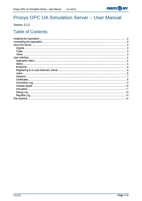
Version: 2.2.2Table of ContentsInstalling the Application (2)Uninstalling the Application (2)About the Server (3)Objects (3)Types (3)Views (3)User Interface (4)Application Menu (4)Status (4)Endpoints (5)Registering to a Local Discovery Server (5)Users (6)Sessions (7)Certificates (8)Connection Log (9)Address Space (10)Simulation (11)Debug Log (12)Reg/Res Log (13)File locations (14)OPC UA Simulation Server is an OPC UA server application, which provides simulated data. You can use it in place of OPC UA servers that provide online production data, for example, to test connections from different OPC UA client applications or to help you with your OPC UA system or application development.Installing the ApplicationThe installation includes a complete “embedded” Java Runtime Environment (JRE). This ensures that you don’t need to install Java in your computer, although the application is running in a Java environment, and you don’t need to worry about the Java updates. The embedded Java is only used for this application.The application install packages are available from upon request. You should get the correct package, depending on your target environment.On Windows, run the installer executable and follow the instructions. By default, the application is installed with normal user privileges under your home directory. If you want to install it to, for ex-ample, Program Files, you need to run the installer as user which has administrator priviledges.On OS X, you can just install it normally from the dmg-package. Just note that the application is not signed, so you need to accept it at the first startup. Since OSX 10.8 (Mountain Lion), this requires that you open the application using the right-click menu - Open. You can then accept the applica-tion to be run, although it is not signed. After the first startup, you can run it normally from the Launch Pad as well.1On Debian-based Linux (such as Ubuntu), usesudo dpkg -i prosys-opc-ua-simulation-server-x.x.x-x.debOn RPM-based Linux (such as Fedora), use usesudo rpm -i prosys-opc-ua-simulation-server-x.x.x-x.x86_64.rpm(If the rpm install fails with "error: failed dependencies" then you are most likely running a Debian-based Linux distribution.)Uninstalling the ApplicationOn Windows the application can be uninstalled through the Control Panel, or with the uninstaller (in the installation folder). Remember to stop the application before uninstalling (some files cannot be removed while the application is running and must be removed manually if uninstalling is done while the application is running).On OS X you can just remove the application from the Applications folder.On Debian-based Linux usesudo dpkg -r prosys-opc-ua-simulation-serverOn RPM-based Linux usesudo rpm -e prosys-opc-ua-simulation-server1 See /Install-Software-from-Unsigned-Developers-on-a-Mac for more information about the Apple Gatekeeper options.About the ServerThe Simulation Server is an OPC UA server that contains simulation signals for demonstration and testing purposes.As most OPC UA servers, the address space of the Simulation Server has three main folders: Ob-jects, Types and Views.Objects include instances of OPC UA nodes, defined in Types folder. Views can include subgroups of OPC UA address spaceThe address space can be explored with the Address Space view. It is also available for all client applications, such as Prosys OPC UA Java Client.See the Address Space part for more about the address space and how to browse it in the server. ObjectsThe Simulation Server defines the following objects:∙Server object is a standard object that provides the status and capability information about the server∙Simulation folder contains all simulation signals defined in the Simulation page∙MyObjects contains a sample object, MyDevice that simulates a simple device with 4 com-ponentso MySwitch is a simple switch variable (DataType=Boolean) that can be turned on and offo MyLevel is a variable (DataType=Double) for simulated level measuremento MyLevelAlarm is an alarm object corresponding to MyLevel. New events are sent from the server when the value of MyLevel exceeds the alarm limits defined in thealarm object.o MyMethod is a sample method that can be called from the client applications ∙MyBigNodeManager represents an object including a large number of data items∙StaticData object includes variables of various data types that change only when they are written toTypesThe OPC UA servers provide complete type information for the objects also in the address space. These can be found from the Types folder. The Simulation Server includes the following types: ∙ObjectTypes includes type definitions for all the objects in the server address space∙VariableTypes includes type definitions for all the variables in the server address space ∙DataTypes defines all the data types that are used in the server address space∙ReferenceTypes defines all the reference types that appear between nodes∙EventTypes define all the events that appear in server address spaceViewsThe Simulation Server does not define any Views.User InterfaceThe user interface of the Simulation Server consists of several views which are organized into tabbed pages.Application MenuThe Application Menu has just a couple of functions, you can shut down the server with File->Shutdown (or you can just close the window). Help->About lists information about the application (e.g. version numbers).StatusThe status page (Figure 1) displays short information about the current server status. If everything is ok, the status displays “Running”. The view also displays the current and starting time of the server. If remote connections are used, you should ensure that the computers are running with synchronized clocks. Especially the secure connections will not work if the clocks are too much out of sync. The Server Status and these times are also available for client application from the Server object.The Connection Addresses show which addresses (URLs) the client applications can use to con-nect to the server. Note that the Simulation Server supports both opc.tcp and https protocols. Most client applications only support opc.tcp, since https was defined recently for OPC UA 1.02. The Simulation Server does not support the soap protocol, which is also an alternative for some (mostly .NET based) OPC UA applications. You can define the available addresses in the Endpoints page. Figure 1: The Status tab displays some basic info about the serverEndpointsThe Endpoints page (Figure 2) allows you to configure all endpoint related settings and view all endpoints that the server has. By clicking “Show all endpoints” button, you see a pop-up window, which displays all the currently defined endpoints. You can edit the settings and save them by click ing “Apply”. The settings are applied the next time the application is started.Figure 2: The Endpoints page allows you to configure the endpoints of the serverRegistering to a Local Discovery ServerThe endpoints page (Figure 2) also has controls for registering the server to a Local Discovery Server. Please see the OPC Unified Architecture specification Part 12 for more information about Local Discovery Server. The view allows enabling/disabling the registration and changing the con-nection address for the Local Discovery Server. Please note that the registration requires a secure connection therefore the discovery server needs to trust Simulation Server’s certificate.UsersThe Users page (Figure 3) displays user authentication settings. OPC UA has multiple options for authentication. Currently only Anonymous and Username/Password configurations are supported. (All user certificates and tokes are actually accepted.). Note! that the changes in User Authentica-tion Methods apply only after restarting the server.You can use the user list to define user names and passwords that are allowed access to the serv-er. Currently all users get equal access rights to the server.Figure 3: Users pageSessionsThe Sessions page (Figure 4) displays the current sessions opened by the client application. The Session list on the left shows the session names and the detail view on the right displays available information about the selected session.Figure 4: Session tab displays all current Sessions in the serverCertificatesOPC UA applications use application instance certificates (not to be confused with user certificates) to authenticate the applications that are allowed to make secure connections (for unsecure con-nections, the certificates are not used).The Certificates page (Figure 5) allows you to define which application certificates you trust. When a new client application connects, its certificate will be added to the certificate list as “Rejected”. This is done by right-clicking the Certificate in the left list and selecting Trust from the menu. You can use the same to later reject a certificate that has been trusted previously.If your operating system has a default application for displaying certificates, you can use that by clicking “Open Certificates in OS viewer”. The certificates are stored in a Certificate Store (PKI folder) in the application settings (See File locations at the end of the manual).Figure 5: Certificates tab allows you to define which certificates you trust.Connection LogThe Connection Log page (Figure 6) displays a history of client connections. The log is stored in an internal database, so it will also show past connections.Figure 6: Connection Log tab displays the connection historyAddress SpaceThe address space of a server includes the data and types that are available for client applications. The address space consists of nodes, which can be objects, variables, various types or views. The nodes are connected to each other with references. The hierarchical references (such as Organiz-es, HasComponent, HasProperty, etc.) are used to compose the tree-structure, which is typically used when displaying the address space. In addition, there can be various non-hierarchical refer-ences (such as HasTypeDefinition, HasCondition, etc.).The Address Space page (Figure 7) can be used to explore the Address Space of the server. You may be familiar with a similar view in some OPC UA Client applications (such as Prosys OPC UA Client or UaExpert). The left part shows the Nodes in a tree view and the right-hand side shows the Attributes and References of the selected node.Figure 7: Address Space of the server. The attributes and references of the selected node are displayed on the right.SimulationThe Simulation page (figure 8) enables configuring custom signals with various simulation wave-forms.“Run Simulation” is used to enable/disable simulation. Interval defines how often the signals are updated. Simulation Time shows the timestamp corresponding to the last update. Simulation can be run in the current time only.The defined signals are displayed on the left. The parameters of the selected signal are configured with the editor on the right-hand side. The parameters depend on the type of the signal.You can add and remove signals using the “+” and “-“-buttons below the signal list. The signal names must be unique. The name is also used to define the NodeId, BrowseName and Display-Name of the signal.The graph on the bottom of the page can be used to visualize the selected signals (the ones that have their Visualize-checkbox checked in the list).Figure 8: Simulation viewExpression signals can be defined with a custom mathematical expression. The expression may also refer to other signals, which are defined with the Inputs parameter. Expression signals cannot be used as inputs for other expressions.Debug LogThe Debug Log page displays logging from the application’s internal behavior. This can be used for examining the application behavior in detail, e.g. if the application is unable to start the server. Figure 9: Debug Log viewReg/Res LogThe Ref/Res Log page can be used to record every request and response to the server (except opening and closing of the secure channel). This functionality is by default off, check the Active checkbox in order to start recording. Note that the recording is kept in memory until cleared by pressing Clear button or shutting down the application, therefore if kept on for very long time, it is possible to run out of memory.Figure 10: Request-Response Log viewFile locationsThe application saves its settings to a folder in path “(user.home)/.prosys/SimulationServer”. The (user.home) is the location of the current user’s home folder. If you want to reset to default se t-tings, just delete the settings file in the folder. Settings are saved automatically when the applica-tion closes. The certificates used in OPC UA communication are saved to PKI –subfolder in the same location.。

ST-500Series Inline PTSA SensorsUser ManualJanuary 10, 2022Rev.3.08Pyxis Lab,Inc.1729Majestic Dr.Suite5Lafayette,CO80026USA©2017Pyxis Lab,Inc.Table of Contents1Introduction 22Specifications 33Unpacking Instrument 33.1Standard Accessories .........................................33.2Optional Accessories .........................................44Installation 54.1ST-500andST-500RO Piping.....................................54.2ST-500SS Piping ............................................64.3Wiring .................................................74.4Connecting via Bluetooth ......................................76.2Connecting via USB ..........................................125Setup and Calibration withuPyxis®Mobile App85.1Download uPyxis®Mobile App ...................................85.2Connecting to uPyxis®Mobile App .................................95.3Calibration Screen andReading...................................105.4Diagnosis Screen ...........................................115.5Device Info Screen ..........................................116Setup and Calibrationwith uPyxis®Desktop App126.1Install uPyxis®Desktop App .....................................126.3Connecting touPyxis®Desktop App ................................136.4Information Screen ..........................................146.5Calibration Screen ..........................................146.6Diagnosis Screen ...........................................157Outputs 157.14–20mA Output Setup ........................................157.2Adjusting 4–20mA Span .......................................167.3Communication using Modbus RTU .................................178Sensor Maintenanceand Precaution178.1Methods to Cleaning the ST-500Series Sensor ..........................178.2Storage .................................................189Troubleshooting1810Contact Us 19Warranty InformationConfidentialityThe information contained in this manual may be confidential and proprietary and is the property of Pyxis Lab,rmation disclosed herein shall not be used to manufacture,construct,or otherwise reproduce the goods rmation disclosed herein shall not be disclosed to others or made public in any manner without the express written consent of Pyxis Lab,Inc.Standard Limited WarrantyPyxis Lab warrants its products for defects in materials and workmanship.Pyxis Lab will,at its option,repair or replace instrument components that prove to be defective with new or remanufactured components (i.e.,equivalent to new).The warranty set forth is exclusive and no other warranty,whether written or oral, is expressed or implied.Warranty TermThe Pyxis warranty term is thirteen(13)months ex-works.In no event shall the standard limited warranty coverage extend beyond thirteen(13)months from original shipment date.Warranty ServiceDamaged or dysfunctional instruments may be returned to Pyxis for repair or replacement.In some in-stances,replacement instruments may be available for short duration loan or lease.Pyxis warrants that any labor services provided shall conform to the reasonable standards of technical com-petency and performance effective at the time of delivery.All service interventions are to be reviewed and authorized as correct and complete at the completion of the service by a customer representative,or des-ignate.Pyxis warrants these services for30days after the authorization and will correct any qualifying deficiency in labor provided that the labor service deficiency is exactly related to the originating event.No other remedy,other than the provision of labor services,may be applicable.Repair components(parts and materials),but not consumables,provided during a repair,or purchased individually,are warranted for90days ex-works for materials and workmanship.In no event will the in-corporation of a warranted repair component into an instrument extend the whole instrument’s warranty beyond its original term.Warranty ShippingA Repair Authorization(RA)Number must be obtained from Pyxis Technical Support before any product can be returned to the factory.Pyxis will pay freight charges to ship replacement or repaired products to the customer.The customer shall pay freight charges for returning products to Pyxis.Any product returned to the factory without an RA number will be returned to the customer.To receive an RMA you can generate a request on our website at https:///request-tech-support/.Pyxis Technical SupportContact Pyxis Technical Support at+1(866)203-8397,*********************,or by filling out a request for support at https:///request-tech-support/.1IntroductionThe Pyxis ST-500Series inline fluorometer sensor measures the concentration of fluorescence tracer PTSA (pyrenetetrasulfonic acid)in water.The standard ST-001Tee Assembly provided with each ST-500/ST-500RO sensor,has two3/4”female NPT ports and can be placed to an existing3/4”sample water line.Pyxis Lab also offers2”and3”Tee formats for larger flow installations.The4–20mA current output of the ST-500Se-ries sensor can be connected to any controller that accepts an isolated or non-isolated4–20mA input.The ST-500Series sensor is a smart device.In addition to measuring fluorescence,the ST-500Series sensor has an extra photo-electric components that monitors the color and turbidity of the sample water.This extra feature allows automatic color and turbidity compensation to eliminate interference commonly associated with real-world waters.The Pyxis ST-500Series sensor has a short fluidic channel and can be easily cleaned.The fluidic and op-tical arrangement of the ST-500Series sensor is designed to overcome shortcomings associated with other fluorometers that have a distal sensor surface or a long,narrow fluidic cell.Traditional inline fluorometers are susceptible to color,turbidity interference,and fouling,making them very difficult to properly clean.The Pyxis ST-500Series sensor uses a narrow wavelength band gallium phosphide photodiode and high temperature-tolerant and humidity-resistant optical filters.This combination greatly enhances the robust-ness of the sensor.It can be operated under a wide range of ambient conditions without the need of humid-ity and temperature regulation.The performance of the ST-500Series sensor can be stable and consistent for a long period of time.2SpecificationsPyxis’s continuous†See Figure4for ST-500SS dimensions.3Unpacking InstrumentRemove the instrument and accessories from the shipping container and inspect each item for any damage that may have occurred during shipping.Verify that all accessory items are included.If any item is missing or damaged,please contact Pyxis Lab Customer Service at*********************.3.1Standard Accessories•Tee Assembly3/4”NPT(1x Tee,O-ring,and Nut)P/N:ST-001*NOTE*ST-001is not included for ST-500SS•7-Pin Female Adapter/Flying Leads Cable(2ft)P/N:MA-1100•User Manual available online at https:///support/3.2Optional AccessoriesThe following optional accessories can be ordered from Pyxis Customer Service(*******************)or Pyxis E-Store at https:///shop/.Figure1.Figure2.4Installation4.1ST-500and ST-500RO PipingThe provided ST-001Tee Assembly can be connected to a pipe system through the3/4”female ports,either socket or NPT threaded.To properly install the ST-500/ST-500RO sensor into the ST-001Tee Assembly,follow the steps below:1.Insert the provided O-ring into the O-ring groove on the tee.2.Insert the ST-500/ST-500RO sensor into the tee.3.Tighten the tee nut onto the tee to form a water-tight,compression seal.Figure3.Dimension of the ST-500/ST-500RO and the ST-001Tee Assembly(mm)4.2ST-500SS PipingThe ST-500SS sensor has3/4”female NPT threaded ports on the sensor itself and therefore does not require a custom tee assembly.It is recommended that two3/4”NPT to1/4”tubing adapters are used to connect the sensor to the sampling system.Sample water entering the sensor must be cooled down to below120°F(49°C).The sensor can be held by a1.75-inch pipe clamp or mounted to a panel with four1/4-28bolts. See Figure4for ST-500SS dimensions.Figure4.Dimension of the ST-500SS(inch)4.3WiringIf the power ground terminal and the negative4–20mA terminal in the controller are internally connected (non-isolated4–20mA input),it is unnecessary to connect the4–20mA negative wire(green)to the4–20mA negative terminal in the controller.If a separate DC power supply other than that from the controller is used, make sure that the output from the power supply is rated for22–26VDC@65mA.*NOTE*The negative24V power terminal(power ground)and the negative4–20mA ter-minal on the ST-500Series sensor are internally connected.Follow the wiring table below to connect the ST-500Series sensor to a controller:ground4.4Connecting via BluetoothA Bluetooth adapter(P/N:MA-WB)can be used to connect a ST-500Series sensor to a smart phone with the uPyxis®Mobile App or a computer with a Bluetooth/USB Adapter(P/N:MA-NEB)and the uPyxis®Desktop App.The power should be sourced from a24VDC power terminal of a controller.If a controller is not available,please purchase a Pyxis PowerPack-1(P/N:MA-BLE-1)or PowerPack-4(P/N:MA-BLE-4)auxiliary power supply with Bluetooth,or an alternative24V power supply that can directly connect to the ST-500 Series sensor with proper cable connectors from Pyxis.Figure5.7-Pin Sensor with MA-WB and uPyxis Mobile5Setup and Calibration with uPyxis®Mobile App 5.1Download uPyxis®Mobile AppDownload uPyxis®Mobile App from Apple App Store or Google Play.Figure 8. uPyxis® Mobile App installation5.2Connecting to uPyxis®Mobile AppConnect the ST-500Series sensor to a mobile smart phone according to the following steps:1.Open uPyxis®Mobile App.2.On uPyxis®Mobile App,pull down to refresh the list of available Pyxis devices.3.If the connection is successful,the ST-500Series and its Serial Number(SN)will be displayed(Figure8).4.Press on the ST-500Series sensor image.Figure9.5.3Calibration Screen and ReadingWhen connected,the uPyxis®Mobile App will default to the Calibration screen.From the Calibration screen,you can perform calibrations by pressing on Zero Calibration,Slope Calibration,and4-20mA Span. Follow the screen instructions for each calibration step.Figure10.5.4Diagnosis ScreenFrom the Diagnosis screen,you can check the diagnosis condition as well as Export&Upload.This feature may be used for technical support when communicating with*********************.To preform a Cleanliness Check,first select the Diagnosis Condition which defines the fluid type that the ST-500Series sensor in currently measuring,then press Cleanliness Check.If the sensor is clean,a Clean message will be shown.If the sensor is severely fouled,a Dirty message will be shown.In this case,follow the procedure in the Methods to Cleaning the ST-500Series Sensor section of this manual.Figure11.5.5Device Info ScreenFrom the Device Info screen.You can name the Device or Product.Figure 12.6Setup and Calibration with uPyxis®Desktop App6.1Install uPyxis®Desktop AppDownload the latest version of uPyxis®Desktop software package from:https:///upyxis/ this setup package will download and install the Framework4.5(if not previously installed on the PC),the USB driver for the USB-Bluetooth adapter(MA-NEB),the USB-RS485adapter(MA-485), and the main uPyxis®Desktop application.Double click the uPyxis.Setup.exe file to install.Figure 13. 7-Pin Sensor with MA-WB and MA-NEB and uPyxis Desktop6.2 Connec t Wing via USBA USB-RS485adapter(P/N:MA-485)can be used to connect a ST-500Series sensor to a computer with the uPyxis®Desktop App.*NOTE*Using non-Pyxis USB-RS485adapters may result in permanent damage of the ST-500Series sensor communication hardware.Figure14.7-Pin Sensor with MA-485 and uPyxis Destop1.Plug the Bluetooth/USB adapter or USB-RS485 adapter into a USB port in the computer.unch uPyxis® Desktop App.3.OnuPyxis® Desktop App, click Device →Connect via USB-Bluetooth or Connect via USB-RS485 (Fig-ure 14).4.If the connection is successful, the ST-500 Series and its Serial Number (SN) will be displayed in the left pane of the uPyxis® window.*NOTE * After the sensor and Bluetooth is powered up, it may take up to 10 seconds for the adapter to establish the wireless signal for communication.Figure 16.Figure 15. uPyxis® Desktop App installationClick Install to start the installation process. Follow the screen instructions to complete the USB driver and uPyxis® installation.6.3 Connecting to uPyxis® Desktop AppConnect the ST-500 Series sensor to a Windows computer using either a Bluetooth/USB adapter (P/N: MA-NEB) or a USB-RS485 adapter (P/N: MA-485) according to the following steps:6.4 Information ScreenOnce connected to the device,a picture of the device will appear on the top-left corner of the window and the uPyxis®Desktop App will default to the Information screen.On the Information screen you can set the information description for Device Name,Product Name,and Modbus Address,then click Apply Settings to save.Figure17.6.5Calibration ScreenTo calibrate the device,click on Calibration.On the Calibration screen there are three calibration buttons, Zero Calibration,Slope Calibration,and4-20mA Span.The screen also displays the reading of the device. The reading refresh rate is every4seconds.Follow the screen instructions for each calibration step.Figure18.6.6 Diagnosis ScreenAfter the device has been calibrated and installation has been completed,to check diagnosis,click on Diag-nosis.When in the Diagnosis screen you can view the Diagnosis Condition of the device.This feature may be used for technical support when communicating with*********************.To preform a Cleanliness Check,first select the Diagnosis Condition which defines the fluid type that the ST-500Series sensor in sensor is clean,a green Clean message will be shown.will be shown.In thiscase,follow the procedure in of this manual.Figure19.7Outputs7.14–20mA Output SetupThe4–20mA output of the ST-500and ST-500SS sensor is scaled as:•PTSA:–4mA=0ppb–20mA=200ppbThe4–20mA output of the ST-500RO sensor is scaled as:•PTSA:–4mA=0ppb–20mA=40ppb7.2Adjusting4–20mA SpanUsers may adjust the output scale using4–20mA Span to change the PTSA value corresponding to the20mA output via uPyxis®.For the uPyxis®Mobile App,press4-20mA Span found on the Calibration and Reading Screen,shown in Figure18.For the uPyxis®Desktop App,click4-20mA Span found on the Calibration Screen,shown in Figure19.Figure 20.Figure 21.*NOTE*Pyxis accommodates custom requests for ST-500/ST-500SS with ranges up to600.0ppb.7.3Communication using Modbus RTUThe ST-500Series sensor is configured as a Modbus slave device.In addition to the ppb PTSA value,many operational parameters,including warning and error messages,are available via a Modbus RTU connection. Contact Pyxis Lab Customer Service(*********************)for more information.8Sensor Maintenance and PrecautionThe ST-500Series sensor is designed to provide reliable and continuous PTSA readings even when installed in moderately contaminated industrial cooling waters.Although the optics are compensated for the effects of moderate fouling,heavy fouling will prevent the light from reaching the sensor,resulting in low readings and the potential for product overfeed if the ST-500Series sensor is used as part of an automated control system.When used to control product dosing,it is suggested that the automation system be configured to provide backup to limit potential product overfeed,for example by limiting pump size or duration,or by alarming if the pumping rate exceeds a desired maximum limit.The ST-500Series sensor is designed to be easily removed,inspected,and cleaned if required.It is sug-gested that the ST-500Series sensor be checked for fouling and cleaned/calibrated on a monthly basis. Heavily contaminated waters may require more frequent cleanings.Cleaner water sources with less con-tamination may not require cleaning for several months.The need to clean the ST-500Series sensor can be determined by the Cleanliness Check using either the uP-yxis®Mobile App(see the Mobile Diagnosis Screen section)or the uPyxis®Desktop App(see the Desktop Diagnosis Screen section).8.1Methods to Cleaning the ST-500Series SensorAny equipment in contact with industrial cooling systems is subject to many potential foulants and contam-inants.Our inline sensor cleaning solutions below have been shown to remove most common foulants and contaminants.A small,soft bristle brush,Q-Tips cotton swab,or soft cloth may be used to safely clean the sensor housing and the quartz optical sensor channel.These components and more come with a Pyxis Lab Inline Probe Cleaning Solution Kit(P/N:SER-01)which can be purchased at our online E-Store https:///product/st-series-probe-cleaning-kit/Figure 22.Inline Probe Cleaning Solution KitTo clean the ST-500Series sensor,soak the lower half of the sensor in100mL inline sensor cleaning solution for30minutes.Rinse the ST-500Series sensor with distilled water and then check for the flashing blue light inside the ST-500Series sensor quartz tube.If the surface is not entirely clean,continue to soak the ST-500 Series sensor for an additional30m e the small,soft bristle brush and Q-Tips cotton swabs as necessary to remove any remaining contaminants in the ST-500Series sensor quartz tube.8.2StorageAvoid long term storage at temperature over140°F.In an outdoor installation,properly shield the ST-500 Series sensor from direct sunlight and precipitation.9TroubleshootingIf the ST-500Series sensor output signal is not stable and fluctuates significantly,make an additional ground connection—connect the clear(shield,earth ground)wire to a conductor that contacts the sample water electrically such as a metal pipe adjacent to the ST-500Series tee.Carry out routine calibration verification against a qualified PTSA standard.After properly cleaning the ST-500Series sensor,carry out the zero point calibration with distilled water and slope calibration using the qualified PTSA s tandard.Pyxis Lab PTSA Standards can be purchased at our online E-Store https:///product/ptsa-standards/Figure23.PTSA100Standard 10Contact UsPyxis Lab,Inc1729Majestic Dr.Suite5Lafayette,CO80026USAPhone:+1(866)203-8397Email:*********************。

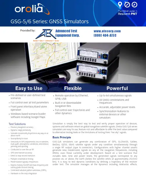
Simulation is simply the best way to test and verif y proper operation of devices, systems and software reliant on global navigation satellite signals. Orolia GSG-5/6 series simulators are easy to use, feature-rich and affordable to offer the best value compared to alternative testing tools or the limitations of testing from “live sky” signals.Basic PrincipleGSG-5/6 simulators can generate any combination o f GPS, GLONASS, Galileo, BeiDou, QZSS, SBAS satellite signals under any condition simultaneously through a single RF output (type N connector). Configurations with higher channel counts generate new, modernized, signals on any of the navigation f requencies, including IRNSS, even those currently under development. Based on a test scenario that includes date, time and power levels, the generated signals correspond to any position on, or above, the earth (below the satellite orbits at approximately 20,000 km). It is easy to test dynamic conditions by defining a trajectory of the receiver under test. The simulator manages all the dynamics including relativistic effects.Test Solutions•Position/navigation accuracy •Dynamic range/sensitivity•Simulate movements/trajectories any way on or above earth •Susceptibility to noise•Sensitivity to GPS impairments: loss of satellites, multi-path, atmospheric conditions, interference, jamming and spoofing •Conducted or over-the-air RF •GPS time transfer accuracy •Effect of leap second transition •Multiple constellation testing •Modernization signals/ frequencies•Keyless military SAASM and dual-frequency and survey-grade receiver testing •Controlled radiation pattern antennas (CRPA)•Hardware-in-the-loop integrationEasy to Use•Pre-defined or user-defined test scenarios•Full control over all test parameters •Front panel interface/stand-alone operation•Windows-based scenario builder software including Google MapsFlexible•Remote operation by Ethernet,GPIB, USB•Built-in or downloadable navigation files•Full control over trajectories and other dynamicsPowerful•Up to 64 simultaneous signals •All GNSS constellations and frequencies•Accurate, adjustable power levels •Synchronization features to external devices or other simulatorsProvided by: (800)404-ATECAdvanced Test Equipment Corp .®Rentals • Sales • Calibration • ServiceSimple Set-up and Operation Even the most inexperienced operator can configure scenarios on the fly without the need for an external PC and pre-compilation phase. Via the front panel, the user can swiftly modify parameters. Each unit comes with a license or GSG StudioView™ Windows sof tware to graphically create, modify, and upload scenarios.A Google Maps inter f ace makes trajectory creation easy. Trajectories can also be defined by recorded or generated NMEA f ormats. Connectivity Extends Ease-of-use and FlexibilityGSG simulators can be controlled via an Ethernet network connection, USB or GPIB. A built-in web interf ace allows complete operation of the instrument through front panel controls. It also allows for file transfers. Connectivity also supports the integration of GNSS simulation into a wide range of other applications. There is an option to control signal generation in real-time through a simple command set. It can synchronize to external systems in many other ways based on its precision timing capabilities and the ability to automatically download ephemeris and almanac data via RINEX files.Input/OutputRF GNSS Signal Generation• Connector: Type N female• DC blocking: Internal, up to 7 VDC; 470 Ω nominal load• Frequency bands:• L1/E1/B1/SAR: 1539 to 1627 MHz• L2/L2C: 1192 to 1280 MHz• L5/E5/B2: 1148 to 1236 MHz• E6/B3:1224 to 1312 MHz• Output channels:• 1 (GSG-51); 4, 8, 16 (GSG-5); 32 (GSG-62),48, (GSG-63), 64 (GSG-64)• Any channel can generate anyconstellation or a derivative signal(multipath, interference, jamming)• Any set of 16 channels can generatewithin a frequency band• Constellations: GPS, GLONASS, Galileo, BeiDou, QZSS, IRNSS• Modulations: BPSK, QPSK, BOC (all)• SBAS: WAAS, EGNOS, GAGAN, MSAS, SAIF (included)• Spurious transmission: ≤40 dBc• Harmonics: ≤40 dBc• Output signal level: -65 to -160 dBm;0.1 dB resolution down to -150 dBm;0.3 dB down to -160 dBm• Power accuracy: ±1.0 dB• Pseudorange accuracy: 1mm• Inter-channel bias: Zero• Inter-channel range: >54 dB • Limits Standard ExtendedAltitude18,240 m(60,000 feet)20,200,000 m(66,273,000 feet)Acceleration 4.0 g No limitsVelocity515 m/s (1000knots)20,000 m/s(38,874 knots)Jerk20 m/s3No limit• White noise signal level: -50 to -160 dBm;0.1 dB resolution down to -150 dBm;0.3 dB down to -160 dBm. ±1.0 dB accuracyExternal Frequency ReferenceInput• Connector: BNC female• Frequency: 10 MHz nominal• Input signal level: 0.1 to 5Vrms• Input impedance: >1kΩFrequency Reference Output• Connector: BNC female• Frequency: 10 MHz sine• Output signal level: 1Vrms in to 50 Ω loadExternal Trigger Input• Connector: BNC female• Level: TTL level, 1.4V nominalXPPS Output• Connector: BNC female• Rate: 1, 10, 100, 1000 PPS (configurable)• Pulse ratio: 1/10 (1 high, 9 low)• Output signal level: Approx. 0V to +2.0V in50 Ω load• Accuracy: Calibrated to ±10 nSec of RFtiming mark output (option to reduce bya factor of ten with a characterization ofoffsets)Built-in TimebaseInternal Timebase – High StabilityOCXO• Aging per 24 h: <5x10-10• Aging per year: <5x10-8• Temp. variation 0…50°C: <5x10-9• Short term stability (Adev @1s): <5x10-12Auxiliary FunctionsInterface• GPIB (IEEE-488.2), USB 1.X or 2.X(SBTMC-488), Ethernet (100/10 Mbps)Settings• Predefined scenarios: User can changedate, time, position, trajectory, numberof satellites, satellite power level andatmospheric model• User defined scenarios: Unlimited• Trajectory data: NMEA format (GGA orRMC messages, or both), convert fromother formats with GSG StudioView™ (seeseparate datasheet)General SpecificationsCertifications• Safety: Designed and tested forMeasurement Category I, Pollution Degree2, in accordance with EN/IEC 61010-1:2001• EMC: EN 61326-1:2013, increased test levelsper EN 61000-6-3:2001 and EN 61000-6-2:2005Dimensions• WxHxD: 210 x 90 x 395 mm(8.25” x 3.6” x 15.6”)• Weight: approx. 2.7 kg (approx. 5.8 lb)Optional Antenna• Frequency: 1000 to 2600 MHz• Impedance: 50 Ω• VSWR: <2:1 (typ)• Connector: SMA male• Dimensions: 15 mm diameter x 36 mmlengthEnvironmental• Class: MIL-PRF-28800F, Class 3• Temperature: 0°C to +50°C (operating);-40°C to +70°C non-condensing @<12,000 m (storage)Humidity:• 5-95 % @ 10 to 30°C• 5-75 % @ 30 to 40°C• 5-45 % @ 40 to 50°CPower• Line Voltage: 100-240 VAC, 50/60/400 H z• Power Consumption: 40 W max.Optional FeaturesRecord and Playback (OPT-RP)This option provides the easiest way to create acomplex scenario by recording satellite signalson a route. It includes a recording receiver andsoftware to automatically generate a simulationscenario that can be modified to ask ‘what if’questions.• True life constellation replication• Automatic scenario generation• Ability to modify signal parameters• Compatible with any recording that includesNMEA 0183 RMC, GGA, and GSV sentencesReal-time Scenario Generator(OPT-RSG)This option supports generation o f 6DOFtrajectory in f ormation via position, velocity,acceleration, or heading commands as theinput f or GPS RF generation. Vehicle attitudeand attitude rate changes, as well as satellitepower levels, are also controllable via real-timecommands.• Control trajectories using 6DOF• Low fixed latency from command input toRF output• Hardware-in-the-loop applications• Includes sensor simulation optionRTK/DGNSS Virtual Reference Station (OPT-RTK)This option supports generation o f RTCM correction data messages for testing an RTK/ Differential-GNSS receiver.• Generates RTCM 3.x correction data via 1002, 1004, 1006, 1010, 1012, and 1033 messages• User settable base station location• Support for GNSS RTK receivers using serial interfacesHigh Velocity Option (OPT-HV) This option extends the limits f or simulated trajectories. As of August 2014, the extended limits are no longer USA export controlled. (See Limits chart under Input/Output specifications.) Jamming Simulation (OPT-JAM) This option extends the capability o f the standard interf erence simulation f eature. Set noise or sweep types of interference and create a location-based jammer to test your system’s susceptibility.• Adjustable bandwidth and amplitude interference• Location-based jamming• Swept-frequency jammingeCall Scenarios (OPT-ECL)This option provides scenarios for testing eCall in vehicle systems per Regulation (EU) 2017/79. Sensor Simulation (OPT-SEN)This option generates sensor data in response to a query according to the trajectory of the GPS RF simulation in real-time. See technical note for more details.• Simultaneously test GPS plus other sensor inputs to your nav system• Simulate data for accelerometers, gravimeters, gyroscopes and odometers UN R144 Test suite (OPT-UNR)This option provides scenarios and test suitefor testing UN R144 in vehicle systems.Ordering InformationBase Configurations• GSG-51: Single channel GPS L1 generator(contact the factory for alternativeconstellations and upgrades to multi-channel and/or frequencies)• GSG-5: 4-channel GPS L1 simulator.Software options increase output channelsto 8 or 16, and adds GLONASS, BeiDou (B1),Galileo (E1), or QZSS constellations. Factoryupgradable to GSG-62 to add more channeland/or frequencies)• GSG-62: 32-channels and up to 2simultaneous frequency bands. Softwareoptions adds GLONASS, BeiDou, Galileo,QZSS or IRNSS constellations; and addssignals on other frequencies (P-code, L2,L2C, Galileo E5a/b, BeiDou B2)• GSG-63: 48-channels and up to 3simultaneous frequency bands. Samesoftware options as GSG-62• GSG-64: 64-channels and up to 4simultaneous frequency bands. Samesoftware options as GSG-62Included with instrument• User manual and GSG StudioView software(one license per unit) on CD• RF cable, 1.5 m• SMA to Type N adapter• USB cable• Certificate of calibration• 3-year warranty1Optional Accessories• Option 01/71: Passive GNSS antenna• Option 22/90: Rack-mount kit• Option 27H: Heavy-duty hard transport case• OM-54: User manual (printed)• Additional StudioView licenses are availableOptional UpgradesConstellations• OPT-GLO: GLONASS Constellation• OPT-GAL: Galileo Constellation• OPT-BDS: BeiDou Constellation• OPT-QZ: QZSS Constellation• OPT-IRN: IRNSS Constellation (requires atleast GSG-62 and OPT-L5)Frequencies (requires at least GSG-62; non-GPS signals are enabled when constellationoption is installed)• Option L2• Option L1C• Option L2C• Option L5• Option L6Channels/Simultaneous Frequencies2• Option 8: 4-channel to 8-channel upgrade• Option 16: 8-channel to 16-channel upgrade• Option 32/2: 16-channel to 32-channel, dualfrequency upgrade• Option 48/3: 32-channel to 48-channel,three frequency upgrade• Option 64/4: 48-channel to 64-channel,four frequency upgradeApplication Packages (typical requirementfor 16 channel min)• OPT-RSG: Real-time scenario generator• OPT-HV: High velocity upgrade to extendedlimits• OPT-RP: Record and playback package• OPT-JAM: Jamming package• OPT-RTK: RTK virtual base station scenarios• OPT-UNR: UN R144 test suite• OPT-ECL: eCall test suiteOptional Services• Calibration/GSG: GSG Calibration Service• Option 95/05: Extended warranty to 5 years• GSG-ASP: GSG Annual Service Plan• GSG-INST: User Training and Installation1Warranty period and available services may vary dependenton country.2Option may require the unit to be returned to factory forupgrade.Configuration Summary03 September, 2021 - GSG-5/6 Series (C)Specifications subject to changeor improvement without notice.© 2021 Orolia。

_PROII⼊门⽤户⼿册（中油奥特--实例部分）编译版权声明P R O I I软件⼊门⽤户⼿册由S I M S C I公司授权，北京中油奥特科技有限公司翻译，本⼿册的全部内容或部分内容均受翻译版权保护，未经本公司许可，任何⼚商或个⼈均不得以任何形式，为其商业⽬的对本⼿册的全部或部分内容擅⾃⾃制、印刷、发⾏。

如有需要可同本公司联系。

因译者⽔平有限，在本书中难免出现错误，敬请读者原谅。

望关⼼P R O I I软件的读者来电来信指导。

北京中油奥特科技有限公司北京西城六铺炕中油招待所2号601 邮编：100011电话：010－82012143 139******** 传真：010－82012142EMAIL aoto@/doc/8f5bd43e0912a2161479293a.htmlHttp: /doc/8f5bd43e0912a2161479293a.html⽬录简介PRO－II能做些什么? 1 模拟中的⼀些状态约定 1 通过这个⼿册能学到什么? 1 如何运⾏? 1 如何得到更多的帮助? 2 问题描述2 如何继续? 2 第⼀部分分离器建⽴流程图（必须） 1.1 定义组份（必须） 1.4 定义⼀个热⼒学⽅法（必须） 1.7 指定⼯艺装置和物流数据（必须） 1.9 运⾏模拟（必须） 1.19 观看运⾏结果 1.19 使⽤闪蒸热键（可选） 1.20 第⼆部分完成膨胀机操作建⽴流程（必须） 2.1 更改物流数据（必须） 2.6 指定⼯艺装置数据（必须） 2.7 运⾏模拟（必须） 2.25 浏览模拟结果 2.26更改模拟缺省值 2.26 第三部分结果介绍改变流程图物流边界条件 3.1 在PFD图上显⽰物性参数 3.4 将PFD图输出到WINDOWS剪贴板上 3.5 在电⼦表格上⽣成物流报告 3.6 为打印PFD图设置页码 3.7 ⽣成图形 3.10 以HTML格式显⽰结果 3.11 缩块图 3.13简介P R O－I I能做些什么?P R O／I I是⼀个在世界范围内应⽤⼴泛的⼯艺模拟软件，在W I N D O W S95、98以及N T 上运⾏。

Excavator Simulation Training InstrumentLesson plan\ Operation Manual\ TroubleshootingJiangsu Hongchang Construction Machinery Co.,LtdContentsExcavator Simulation Training InstrumentLessonPlanJiangsu Hongchang ConstructionMachinery Co.,LtdTraining OutlineWe recommend that you operate the instrument and train students according to the following training outline in order to make full use of the simulation instrument, and you can also modify and add the contents for reaching the optimum training effect.1. Training items are total 22 lessons, they contains: training mode, test mode and entertainment mode.The training mode is the basic training lesson, it asks students to learn and operate the instrument firstly. Students can master the basic knowledge of excavator, such as, 8 movements of 2 control levers, the safety notes and skills through 11 lessons.The test mode designs 7 practical working items of excavator. Students must operate the first item qualifiedly then enter the next item, which ask students to be proficient in operation.The entertainment mode adopts some games to train students mastering the operation skills and contain education in amusement. In this mode, students finish some interesting items with various difficulties by controlling the boom, arm, bucket.2. The training items are arranged in the sequence from simple to complex, students should operate the first items, such as Free Movements and loading example, so that they can be proficient in the 8 movements of 2 control levers. Only building up a solid basis, students can finish the variously difficult items in the next stage because all kinds of excavator works ask operators must be skillful in the operation of 2 control levers.3. The aim of simulation instrument is to convert the first 5-10 hours training on the real excavator into the 30-50 hours training on the simulation instrument, which ensures students to master the 2 control levers, and saves the training cost for school, reduces the wear of real excavator and fuel consumption.4. In the process of training simulation instrument, the teacher should correct students’errors in time, and discipline students to operate the instrument in accordance with the practical operation rules and notes of excavator, this is to make students master the skills and safety notes of real excavator through the simulation instrument, students can standardize operation in the real excavator in the future.5. School should arrange students to read, write down and recite the safety notes and skills of excavator in the theory files.6. The teacher should be strict with students for they master the excavator operation, skills and notes, and laying the foundation for the future real excavator training, saving the training cost and improving the teaching quality.The First Stage: Teaching Section of Simulation InstrumentLessons ArrangementsClass Time: 5-8 ClassesTeaching Aim: Comprehend and master the preliminary functions of 2 control levers and excavator basic operations and skills.Class Arrangements: 1. Class Meeting；2. Item Arrangements;3. Summary;Detailed Teaching Plans：I. Class Meeting；(1)．Students register after entering classroom, the teacher tells students theclassroom disciplines and notes.(2)．Introduce each operational buttons.(3)．Introduce the teaching functions and aims of simulation instrument.①The simulation instrument is specially designed and manufactured for training the excavator driver. The operation of 2 control levers is the same with the real excavator (be able to switch the forehand or backhand). The instrument has the lifelike pictures, various sound and language hints. Students can be familiar with the excavator skills through simulation training, then go on the practical operation on the real excavator, which help students master the excavator skills and become a qualified driver.②During operating, not allow students to replace the items privately, they should strictly follow the appointed items and class time to operate, and keep the stable, correct, and light operation in stead of rude operation.(4). When operating the simulation instrument, students can watch the videos of real excavator according to the different items in order to know the operational contents and standard movements. The teacher introduces the excavator’s structures, components names and usages, working environments for students. Before operating, students should know the meanings of 2 labels sticking on the 2 control boxes and remember the 8 movements of 2 control levers. (tips: imagine excavator as people, ie. boom is the upper arm of people, arm is the lower arm, bucket is the hand, bucket teeth are the fingers, this is to be easily understand). Students can remember and answer the left/right control levers’ positions and functions, which is useful to operate smoothly and lay the foundation for the next items.(5). Requirements: Students should remember the movements of 2 control levers and their functions.(6). Watch and record the Power Point from the help files for masteringoperational skills and safety knowledge.II. Item ArrangementsItem Contents: Rudiment Learning – Free MovementsClass Time：3-5 classesClass Requirements: ask students to master the basic and compound operation of 2control levers.Teaching Plans:Free Movements1．Select the item through operating the simulation instrument.2．The teacher instructs the operational methods and functions of left/right levers.3．Firstly, arrange students to practice a single movement of left/right levers, for example, pulling the right control lever back is to raise the boom; pulling to the left is to close the bucket. Let students know and practice each single movement of 2 control levers, then go on the compound operation until they are really proficient in 8 movements.4. Operate the boom, arm and bucket to support one side of excavator for letting students know when the excavator need be support and the safety notes after supporting.5. Firstly, the teacher make the operational examples, (the teacher should instruct students while operating, so that students are easily to accept and understand). Students can operate the control levers up, down, left, right by themselves after watching teacher’s example. Don’t stamp on the pedals.Firstly, pull the right control lever back to raise boom and watch the pictures on computer, know each direction of control lever presents the movement name andfunction. During operating, don’t produce the sound when arm cylinder strikes bucket cylinder at the end of piston. When cylinder piston is near, the piston rod should keep 5-10 cm clearance. After mastering each movement of 2 control levers, park the machine properly.6. Use the 2 pedals to travel. Before traveling, students should know the meanings of front/rear travel devices. The teacher instructs the different controls and notes when front idler is in front or rear of travel device. Students master how to properly travel and know the safety knowledge of travel.7. Prepare for traveling. Firstly raise boom, fully roll out the arm cylinder and bucket cylinder, after that, lower boom, keep bucket 40-50cm above the ground. 2 feet lightly stamp the pedals, (reminding: know the systems of excavator, the front is front idler, the back is driving tumbler before traveling by pedals), 2 feet stamping forward is to travel forward, 2 feet stamping backward is to travel backward; Lifting left foot (when pedal is median), right foot stamps forward or backward, the excavator will travel forward and turn left or backward and turn left; Lifting right foot (when pedal is median), left foot stamps forward or backward, the excavator will travel forward and turn right or backward and turn right. If need turn where the excavator is, one foot stamps pedal forward, another stamps pedal backward.8. Pull the left control lever left or right, the excavator rotate 180°, then stop the control lever. Experience the pedals again. The cab facing the direction of front idler, stamp the pedal forward if need travel forward; the cab facing the direction of driving tumbler, stamp the pedal backward if need travel forward. Why? Please think over. Because the under carriage of excavator don’t change direction, but the upper structure has changed the direction, the control lever also has changed the direction with upper structure, students should ensure the direction before traveling. (Avoid dangers on the real excavator).Note: In the item of free movements, the excavator only travel in the green area. In all items, the pictures will appear the red flash, words and sound information if happen the wrong operation, for example, the bucket touches the track or any part of excavator. (If appear the above information, please check the cause and properly operate)After students are proficient in free movements, the teacher gives the commands according to the pictures for checking students the corresponding operations. After finish practicing, park the excavator properly.Requirements: When stamping the pedals, should be lightly stamp or lightly lift. Be familiar with the functions, notes and operations of control levers and pedals. Be clear about the front or back directions of excavator.9. The pictures are simple, but students can be proficient in operating 2 control levers through keeping practicing. Only mastering the 2 control levers, students can finish the future items successfully.Item Contents：Rudiment Learning— Loading ExampleClass Time：4-10 ClassesClass Requirements: Be proficient in the basic operation of loading and unloading Teaching Plans：Loading Example1．This item is a great help to operate the real excavator, so arrange students to practice more in order to master loading.2．This item contents：Following the green line to operate the left, right control levers, this is a single movement practice of digging soil and loading. Student should learn the whole process from the bucket opening to closing according to the standard movements. After mastering the basic loading movements, students can freely choose digging sand and loading.3. Details: Following the loading example to keep practicing for master the basic movements of digging and loading.4. The teacher should check students’operations for being standard. Students should pay attention to roll in the arm to the correct position and keep the bucket horizontal. Check the bucket for leaking soil or hitting other objects.Requirements: operate smoothly, correctly, lightly, but not too fast.5. The teacher should correct the problems: don’t lower the boom, don’t roll in arm, the bucket isn’t full. And instruct the safety notes of the real excavator operation. For example:①When unloading, the bucket is not beyond the truck and personnel.②Try to r otate excavator in a small angle for raising working efficiency.③ Be careful that dump soil from the suitable height for avoiding to damage trucks.④ Loading should start from the front of truck to the back, or start from the middle to 2 sides of truck, keep the loads uniform.6. In this item, the truck will automatically leave after taking the 10000Kg loads, the next truck will drive to the loading position for keeping operation.7. Note: if the picture flashes one time, 5 points will be deducted. The possible causes are hitting truck or leaking sand out of truck. If the loads were leaked out of truck, the truck wouldn’t drive, even damage, so the safety points on pictures don’t less than 80 points.III、Summary；1. The teacher makes the summary of occurred problems.①During digging sand, students haven’t rolled in the arm to the correct position, haven’t kept the bucket horizontal.②Operated so fast that the movement wasn’t standard.2. Students write a self-evaluation about the occurred problems, wrong operations and how to correct in the next training.Class Arrangements：1. Class Meeting；2. Item Arrangements；3. Summary；Detailed Teaching Plans：1、Class Meeting；1．The teacher reads students’self-evaluation for finding out and solving the common problems.Example 1: Students have not gained an adequate understanding of simulation instrument, or think it as a game.The teacher: The simulation instrument is specially designed for training excavator, not a simple game. It can help students have a perceptual knowledge about excavator through training before operating the real excavator, and help master the operational skills, so students must correct the attitude to perform a training exercises, only do this, students can master the excavator operation faster and better.Example 2: The movements of digging sand aren’t standard, the operations of arm and bucket aren’t proper.The teacher: Don’t operate too fast on simulation instrument, follow the examples to do standard, properly. Students should keep practicing until master movements.2. Ask students don’t replace the operational items privately.2、Item Arrangements；Item Contents：Rudiment Learning—90°digging and dumpingClass Time：5-8 classesRequirements：1．Master the skill and notes of digging and dumping.2. Be proficient in the match of 2 control levers and skills.3. Ask student dump through the simple, compound operations.Teaching Plans：90° Digging and DumpingTeaching Plans：Traveling and LoadingUp and Down Trailer。