10宏观经济学英文版(多恩布什)课后习题答案全解
- 格式:doc
- 大小:100.00 KB
- 文档页数:12


第4章增长与政策一、概念题1.绝对趋同(absolute convergence)答:绝对趋同是指不论各国的其他特征如何,穷国的人均收入增长倾向于比富国更快。
从理论上说,经济趋同可分为“绝对趋同”和“条件趋同”两种,但实证研究证明绝对趋同并不存在,而无论是在理论上,还是在现实世界中,条件趋同都是客观存在的现象。
2.规模报酬递增(increasing returns to scale)答:规模报酬递增指产量增加的比例大于各种生产要素增加的比例。
设生产函数为Q =f(L,K),则当劳动和资本投入量同时增大λ倍时,产量为aQ=f(λL,λK),a>λ表示产量增加的幅度要大于要素投入的增长幅度。
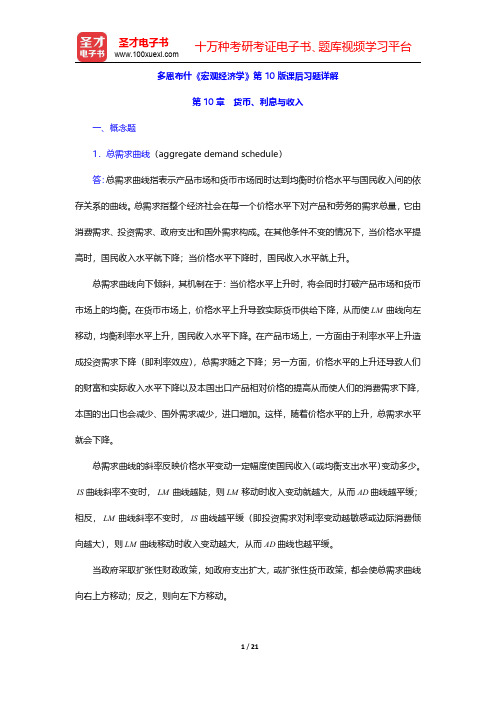
规模报酬递增的生产函数,总产量曲线凸向右下方,表示产量的增加幅度大于要素投入量的增加幅度,如图4-1所示。
图4-1 规模报酬递增图4-1中,横轴表示劳动L和资本投入量K,纵轴表示产量Q,曲线Q为总产量曲线。
当各种要素投入量由X1增加到X2时,引起产量由Q1增加到Q2,要素投入量增加了一倍,而产量的增加大于一倍。
产生规模报酬递增的主要原因是企业生产规模扩大所带来的生产效率的提高。
它可以表现为:生产规模扩大以后,企业能够利用更先进的技术和机器设备等生产要素,而较小规模的企业可能无法利用这样的技术和生产要素。
随着对较多的人力和机器的使用,企业内部的生产分工能够更加合理和专业化。
此外,人数较多的技术培训和具有一定规模的生产经营管理也可以节省成本。
3.稳定均衡(stable equilibrium)答:稳定均衡指如果经济体系的均衡状态遭到暂时破坏时,依靠其自身的力量最终还会恢复到原来所处的均衡状态的一种均衡。
其特点是一个经济体系的均衡状态,在制约它的各种外部条件发生变动时,会使该经济体系产生脱离均衡状态的运动,但是,经济体系内部又同时会自动地产生一种力量,这种力量使体系中的各种变量重新恢复到原来的均衡状态。
例如,当某一商品的供给曲线在均衡点的斜率大于需求曲线的斜率时,脱离均衡状态的波动幅度会自动逐渐缩小以至消失,并最终停留在原均衡点上,这就是阐述动态均衡的蛛网理论所描述的收敛型蛛网情况。

多恩布什《宏观经济学》第10版课后习题详解第20章国际调整与相互依存一、概念题1.自动调节机制(automatic adjustment mechanisms)答:自动调节机制指自动起作用消除国际收支失衡问题的机制。
在纯粹的自由经济中有货币—价格机制、收入机制及利率机制等国际收支自动调节机制。
货币—价格机制,也称“价格—现金流动机制”,其描述的是国内货币供给存量与一般物价水平变动以及相对价格水平变动对国际收支的影响。
当一国处于逆差状态时,对外支付大于收入,货币外流,物价下降,本国汇率也下降,由此导致本国出口商品的价格绝对或相对下降,从而出口增加,进口减少,贸易收入得到改善。
收入机制的调节作用表现为:当国际收支逆差时,国民收入下降。
国民收入下降引起社会总需求下降,从而进口需求也下降,进而改善贸易收支。
利率机制的调节作用表现为:当国际收支发生逆差时,本国货币供给存量减少,利率因此上升,这意味着本国金融资产的收益上升,从而对本国金融资产的需求上升,对外国金融资产的需求相对下降。
这样,资金外流减少或内流增加,资本与金融项目收支得到改善。
当国际收支顺差时,上述的自动调节仍然起作用,只是方向相反而已。
2.内部和外部平衡(internal and external balance)答:内部平衡指国民经济处于无通货膨胀的充分就业状态。
内部均衡时国内产品市场、货币市场和劳动市场同时达到均衡,宏观经济处于充分就业水平上,并且没有通货膨胀的压力,经济稳定增长。
内部均衡目标包括经济增长、价格稳定和充分就业。
外部均衡指国际收支平衡,也即贸易品的供求处于均衡状态。
当国际收支平衡时,既无国际收支顺差,也无国际收支逆差。
在开放经济中,宏观经济的最终目标是实现内部均衡和外部均衡。
英国经济学家詹姆斯·米德开创性地提出了“两种目标、两种工具”的理论模式,即在开放经济条件下,一国经济如果希望同时达到对内均衡和对外均衡的目标,则必须同时运用支出增减政策和支出转换政策两种工具。
宏观经济学第二章概念题1.如果政府雇用失业工人,他们曾领取TR美元的失业救济金,现在他们作为政府雇员支取TR美元,不做任何工作,GDP会发生什么情况?请解释。
答:国内生产总值指一个国家(地区)领土范围,本国(地区)居民和外国居民在一定时期内所生产和提供的最终使用的产品和劳务的价值。
用支出法计算的国内生产总值等于消费C、投资I、政府支出G和净出口NX之和。
从支出法核算角度看:C、I、NX保持不变,由于转移支付TR美元变成了政府对劳务的购买即政府支出增加,使得G增加了TR美元,GDP会由于G的增加而增加。
2.GDP和GNP有什么区别?用于计算收入/产量是否一个比另一个更好呢?为什么?答:(1)GNP和GDP的区别GNP指在一定时期内一国或地区的国民所拥有的生产要素所生产的全部最终产品(物品和劳务)的市场价值的总和。
它是本国国民生产的最终产品市场价值的总和,是一个国民概念,即无论劳动力和其他生产要素处于国内还是国外,只要本国国民生产的产品和劳务的价值都记入国民生产总值。
GDP指一定时期内一国或地区所拥有的生产要素所生产的全部最终产品(物品和劳务)的市场价值的总和。
它是一国范围内生产的最终产品,是一个地域概念。
两者的区别:在经济封闭的国家或地区,国民生产总值等于国内生产总值;在经济开放的国家或地区,国民生产总值等于国内生产总值加上国外净要素收入。
两者的关系可以表示为:GNP=GDP+[本国生产要素在其他国家获得的收入(投资利润、劳务收入)-外国生产要素从本国获得的收入]。
(2)使用GDP比使用GNP用于计量产出会更好一些,原因如下:1)从精确度角度看,GDP的精确度高;2)GDP衡量综合国力时,比GNP好;3)相对于GNP而言,GDP是对经济中就业潜力的一个较好的衡量指标。
由于美国经济中GDP和GNP的差异非常小,所以在分析美国经济时,使用这两种的任何一个指标,造成的差异都不会大。
但对于其他有些国家的经济来说明,这个差别是相当大的,因此,使用GDP作为衡量指标会更好。

多恩布什宏观经济学第十版课后习题答案02CHAPTER 2Solutions to Problems in the Textbook:Conceptual Problems:1. Government transfer payments (TR) do not arise out of anyproduction activity and are thus not counted in the value of GDP. If the government hired the people who currently receive transfer payments, then their wages would be counted as part of government purchases (G), which is counted in GDP. Therefore GDP would rise.2.a. If the firm buys a car for an executive's use, the purchase counts asinvestment (I). But if the firm pays the executive a higher salary and she then buys a car, the purchase is counted as consumption (C).2.b. The services that a homemaker provides are not counted in GDP(regardless of their value). However, if an individual officially hires his or her spouse to perform household duties at a certain wage rate, then the wages earned will be counted in GDP and GDP will increase.2.c. If you buy a German car, consumption (C) will increase but netexports (NX = X - Q) will decrease. Overall GDP will increase by the value added at the foreign car dealership, since the import price is likely to be less than the sales price. If you buy an American car, consumption and thus GDP will increase. (Note: If the car you buy comes out of the car dealer's inventory, then the increase in C will bepartially offset be a decline in I, and GDP will again only increase by the value added.)3. GDP is the market value of all final goods and services currentlyproduced within the country. (The U.S. GDP includes the value of the Hondas produced by a Japanese-owned assembly plant that is located in the U.S., but it does not include the value of Nike shoes that are produced by an American-owned shoe factory located in Malaysia.) GNP is the market value of all final goods and services currently produced using assets owned by domestic residents. (Here the value of the Hondas produced by a Japanese-owned Honda plant is not counted but the value of the Nikes by the American-owned shoe plant is.) Neither is necessarily a better measure of the output of a nation.The actual value of the GDP and GNP for the U.S. is fairly close.4. The NDP (net domestic product) is defined as GDP minusdepreciation. Depreciation measures the value of the capital that wears out during the production process and has to be replaced. Therefore NDP comes closer to measuring the net amount of goods produced in this country. If this is what you want to measure, then NDP should be used.5. Increases in real GDP do not necessarily mean increases in welfare.For example, if the population of a country increases by more than real GDP, then the population of the country is on average worse off.Also some increases in output come from welfare reducing events. For example, increased pollution may cause more lung cancer, and the treatment of the lung cancer will contribute toGDP. Similarly, an increase in crime may lead to overtime work for police officers, whose increased salary will increase GDP. But the welfare of the people in the country may not have increased in either case. On the other hand, GDP does not always accurately measure quality improvements in goods or services (faster computers or improved health care) that improve people's welfare.6. The CPI (consumer price index) and the PPI (producer price index)are both measured by looking at a certain market basket. The CPI's basket contains mostly finished goods and services that consumers tend to buy regularly in their daily lives. The PP I’s basket contains raw materials and semi-finished goods, that is, it measures costs to the producer of a product and its first user. The CPI is a concurrent economic indicator, whereas the PPI is a leading economic indicator.7. T he GDP-deflator is a price index that covers the average priceincrease of all final goods and services currently produced within an economy. It is defined as the ratio of current nominal GDP to current real GDP. Nominal GDP is measured in current dollars, while real GDP is measured in so-called base-year dollars. Even though early estimates of the GDP-deflator tend to be unreliable, the GDP-deflator can be a more useful price index than the CPI or PPI (both of which are fixed market baskets). This is true for two reasons: first it measures a much wider cross-section of goods and services; second, a fixed market basket cannot account for people substituting away from goods whose relative prices have changed, while the GDP-deflator, which includes all goods and services produced within the country, can.8. If nominal GDP has suddenly doubled, it is most likely due to anincrease in the average price level. Therefore, the first thing you would want to check is by how much the GDP-deflator has changed, to calculate by how much real output (GDP) has changed. If nominal GDP and the GDP-deflator have both doubled, then real GDP should be the same.9. Assume the loan you made yields you an annual nominal return of 7%.If the rate of inflation is 4%, then your rate of return in real terms isonly 3%. If, on the other hand, if inflation rate is 10%, then you will actually get a negative real rate of return, that is, you will lose 3% of your purchasing power. One way to protect yourself against such a loss of purchasing power is to adjust the interest rate for inflation, that is, to index the loan. In other words, you can require that, in addition to the specified interest rate of the loan of, let’s say, 3%, the borrower also has to pay an inflation premium equal to the percentage change in the CPI. In this case, a real rate of return of 3% would be guaranteed.Technical Problems:1. The text calculates the change in real GDP in 1992 prices in thefollowing way:[RGDP01- RGDP92]/RGDP92= [3.50 - 1.50]/1.50 = 1.33 = 133%.To calculate the change in real GDP in 2001 prices, we first have to calculate the GDP of 1992 in 2001 prices. Thus we take the quantities consumed in 1992 and multiply them by the prices of 2001, as follows:Beer 1 at $2.00 = $2.00Skittles 1 at $0.75 = $0.75_______________________________Total $2.75The change in real GDP can now be calculated as[6.25 - 2.75]/2.75 = 1.27 = 127%.We can see that the growth rate of real GDP calculated this way is roughly the same as the growth rate calculated above.2.a. The relationship between private domestic saving, investment, thebudget deficit and net exports is shown by the following identity:S - I ≡ (G + TR - TA) + NX.Therefore, if we assume that transfer payments (TR) remain constant, then an increase in taxes (TA) has to be offset either by an increase in government purchases (G), a decrease in net exports (NX), or a decrease in the difference between saving (S) and investment (I).2.b. From the equation YD ≡C + S it follows that an increase indisposable income (YD) will be reflected in an increase in consumption (C), saving (S), or both.2.c. From the equation YD ≡ C + S it follows that when eitherconsumption (C) or saving (S) increases, disposable income (YD) must increase as well.3.a. Since depreciation D = I g - I n = 800 - 200 = 600 ==>NDP = GDP - D = 6,000 - 600 = 5,4003.b. From GDP = C + I + G + NX ==> NX = GDP - C - I - G ==>NX = 6,000 - 4,000 - 800 - 1,100 = 100.3.c. BS = TA - G - TR ==> (TA - TR) = BS + G ==> (TA - TR) = 30 +1,100 = 1,1303.d. YD = Y - (TA - TR) = 5,400 - 1,130 = 4,2703.e. S = YD - C = 4,270 - 4,000 = 2704.a. S = YD - C = 5,100 - 3,800 = 1,3004.b. From S - I = (G + TR - TA) + NX ==> I = S - (G + TR - TA) - NX= 1,300 - 200 - (-100) = 1,200.4.c. From Y = C + I + G + NX ==> G = Y - C - I - NX ==>G = 6,000 - 3,800 - 1,200 - (-100) = 1,100.Also: YD = Y - TA + TR ==> TA - TR = Y - YD = 6,000 - 5,100 ==> TA - TR = 900From BS = TA - TR - G ==> G = (TA - TR) - BS = 900 - (-200) ==> G = 1,1005. According to Equation (2) in the text, the value of total output (inbillions of dollars) can be calculated as: Y = labor payments + capital payments + profits = $6 + $2 + $0 = $86.a. Since nominal GDP is defined as the market value of all final goodsand services currently produced in this country, we can only measure the value of the final product (bread), and therefore we get $2 million (since 1 million loaves are sold at $2 each).6.b. An alternative way of measuring total GDP would be to calculate allthe value added at each step of production. The total value of the ingredients used by the bakeries can be calculated as: 1,200,000 pounds of flour ($1 per pound) = 1,200,000100,000 pounds of yeast ($1 per pound) = 100,000100,000 pounds of sugar ($1 per pound) = 100,000100,000 pounds of salt ($1 per pound) = 100,000________________________________________________________ __= 1,500,000Since $2,000,000 worth of bread is sold, the total value added at the bakeries is $500,000.7. If the CPI increases from 2.1 to 2.3, the rate of inflation can becalculated in the following way:rate of inflation = (2.3 - 2.1)/2.1 = 0.095 = 9.5%The CPI often overstates inflation, since it is calculated by using afixed market basket of goods and services. But the fixed weights in the CPI's market basket cannot capture the tendency of consumers to substitute away from goods whose relative prices have increased.Therefore, the CPI will overstate the increase in consumers' expenditures.8.The real interest rate (r) is defined as the nominal interest rate (i)minus the rate of infla tion (π). Therefore the nominal interest rate is the real interest rate plus the rate of inflation, ori = r + π = 3% + 4% = 7%.。
第24章前沿课题一、概念题1.GDP的周期成分(cyclical component of GDP)答:GDP的周期性成分指产出围绕其增长趋势的波动,即经济波动或经济周期。
经济增长的过程就是总体经济活动的扩张和收缩交替反复出现的过程。
一个完整的经济周期包括繁荣、衰退、萧条、复苏(也可以称为扩张、持平、收缩、复苏)四个阶段。
在繁荣阶段,经济活动全面扩张,不断达到新的高峰。
在衰退阶段,经济短时间保持均衡后出现紧缩的趋势。
在萧条阶段,经济出现急剧的收缩和下降,很快从活动量的最高点下降到最低点。
在复苏阶段,经济从最低点恢复并逐渐上升到先前的活动量高度,进入繁荣。
2.菜单成本(menu cost)答:菜单成本指企业为改变销售商品的价格,需要给销售人员和客户提供新的价目表所花费的成本,类似于饭馆改变价格重新制作菜单所产生的成本。
它是新凯恩斯主义为反击新古典主义的批判并证明其所主张的价格黏性的重要理由。
关于菜单成本能否引起价格的短期黏性,经济学家们的观点是不一致的。
一部分经济学家认为,菜单成本通常非常小,不可能对经济产生巨大影响。
另一部分经济学家却认为,菜单成本虽然很小,但由于总需求外部性的存在,会导致名义价格出现黏性,从而对整个经济产生巨大影响,甚至引起周期性波动。
3.理性预期(rational expectations)答:理性预期又称合理预期,指在有效地利用一切信息的前提下,对经济变量作出的从长期来看最为准确的,又与所使用的经济理论、模型相一致的预期。
约翰·穆思在其《合理预期和价格变动理论》一文中首先提出这一概念,其含义有三个:①作出经济决策的经济主体是有理性的。
②所作决策为正确决策,经济主体会在作出预期时力图获得一切有关的信息。
③经济主体在预期时不会犯系统性错误。
即使犯错误,他也会及时有效地进行修正,使得在长期而言预期保持正确。
它是新古典宏观经济理论的重要假设(其余三个为个体利益最大、市场出清和自然率),是新古典宏观经济理论攻击凯恩斯主义的重要武器。
第5篇重大事件、国际调整和前沿课题第19章重大事件:萧条经济学、恶性通货膨胀和赤字一、简答题1.恶性通货膨胀对宏观经济运行效率将产生哪些不利影响?答:恶性通货膨胀对宏观经济运行效率产生的不利影响主要包括:(1)恶性通货膨胀使价格信号扭曲,使厂商无法根据价格提供的信号来决策,造成经济活动的低效率。
(2)恶性通货膨胀使厂商必须经常性地改变其产品或服务的价格,产生因价格改变而发生的菜单成本。
(3)恶性通货膨胀使不确定性提高,引发资源配置向通货膨胀预期有利的领域倾斜,不利于经济的长期稳定发展。
(4)恶性通货膨胀降低人们的货币需求,这会使往返银行的次数增多,以至于磨掉鞋底,经济学上这种成本被称为“鞋底成本”。
2.为什么通货膨胀有通货膨胀税的说法?它与铸币税是一回事吗?答:(1)如果货币供给的增加触发物价上涨,导致通货膨胀,由于通货膨胀的再分配效应,势必削弱社会公众手中所持有货币的购买力,引起一部分货币购买力从社会公众向货币发行者转移,这种转移犹如一种赋税,因而被称为通货膨胀税。
(2)铸币税指的是政府凭借对货币发行权的垄断而获得的对一部分社会资源的索取权,铸币税的数额等于所发行的货币面值与其实际发行成本之间的差额,实际发行成本主要包括纸张成本及印制费等。
通货膨胀税与铸币税不是一回事,只要政府发行的货币面值与发行成本之间存在差额,则必定存在铸币税;但如果所发行的货币恰好为经济活动所需要,没有相应出现通货膨胀,则就不存在通货膨胀税;只有在过度发行货币引致通货膨胀的时候,才会存在通货膨胀税。
3.预算赤字是个问题吗?为什么是?或者为什么不是?答:预算赤字是在编制预算时支出大于收入的差额,是计划安排的赤字。
预算赤字是个问题。
原因分析如下:(1)在短期,扩张性财政政策引起的赤字增加会刺激总需求,使产出增加。
但同时利率上升会挤出私人消费和投资,而资本积累的降低意味着未来经济增长的乏力。
(2)在开放经济中,预算赤字增加会提高利率,吸引国外资金流入并使本币升值,削弱了本国商品的竞争力,使国际收支的经常项目恶化。
Chapter 5Solutions to the Problems in the TextbookConceptual Problems:1. The aggregate supply curve shows the quantity of real total output that firms arewilling to supply at each price level. The aggregate demand curve shows all combinations of real total output and the price level at which the goods and the money sectors are simultaneously in equilibrium. Along the AD-curve nominal money supply is assumed to be constant and no fiscal policy change takes place.2. The classical aggregate supply curve is vertical, since the classical model assumes thatnominal wages adjust very quickly to changes in the price level. This implies that the labor market is always in equilibrium and output is always at the full-employment level.If the AD-curve shifts to the right, firms try to increase output by hiring more workers, who they try to attract by offering higher nominal wages. But since we are already at full employment, no more workers can be hired and firms merely bid up nominal wages. The nominal wage increase is passed on in the form of higher product prices. In the end, the level of wages and prices will have increased proportionally, while the real wage rate and the levels of employment and output will remain unchanged.If there is a decrease in demand, then firms try to lay off workers. Workers, in turn, are willing to accept lower wages to stay employed. Lower wage costs enable firms to lower their product prices. In the end, nominal wages and prices will decrease proportionally but the real wage rate and the level of employment and output will remain the same.3. There is no single theory of the aggregate supply curve, which shows the relationshipbetween firms' output and the price level. A number of competing explanations exist for the fact that firms have a tendency to increase their output level as the price level increases. The Keynesian model of a horizontal aggregate supply curve supposedly describes the very short run (over a period of a few months or less), while the classical model of a vertical aggregate supply curve is supposed to hold true for the long run (a period of more than 10 years). The medium-run aggregate supply curve is most useful for periods of several quarters or a few years. This upward-sloping aggregate supply curve results from the fact that wage and price adjustments are slow and uncoordinated. Chapter6 offers several explanations for the fact that labor markets do not adjust quickly. Theseinclude the imperfect information market-clearing model, the existence of wage contracts or coordination problems, and the fact that firms pay efficiency wages and price changes tend to be costly.4. The Keynesian aggregate supply curve is horizontal since the price level is assumed to befixed. It is most appropriate for the very short run (a period of a few months or less). The classical aggregate supply curve is vertical and output is assumed to be fixed at its potential level. It is most appropriate for the long run (a period of more than 10 years) when prices are able to fully adjust to all shocks.5. The aggregate supply and aggregate demand model used in macroeconomics is notvery similar to the market demand and market supply model used in microeconomics.While the workings of both models (the distinction between shifts of the curves versus movement along the curves) are similar, these models are really unrelated. The "P" in the microeconomic model stands for the relative price of a good (or the ratio at which two goods are traded), whereas the "P" in the macroeconomic model stands for the average price level of all goods and services produced in this country, measured in money terms.Technical Problems:1.a. As Figure 5-9 in the text shows, a decrease in income taxes will shift both the AD-curveand the AS-curve to the right. The shift in the AD-curve tends to be fairly large and, in the short run (when prices are fixed), leads to a significant increase in output without a change in prices. In the long run, the AS-curve will also shift to the right--since lower income tax rates provide an incentive to work more--but only by a fairly small amount.Therefore we see a slightly higher real GDP with a large increase in the price level in the long run.1.b. Supply-side economics is any policy measure that will increase potential GDP by shiftingthe long-run (vertical) AS-curve to the right. In the early 1980s, supply-side economists put forth the view that a cut in income tax rates would increase the incentive to work, save and invest. This would increase aggregate supply so much that the inflation and unemployment rates would simultaneously decrease. The resulting high economic growth might then even lead to an increase in tax revenues, despite lower tax rates. However, these predictions did not become reality. As seen in the answer to 2.a., the long-run effect of a tax cut on output is not very large, although it can increase long-term output to some degree.2.a. According to the balanced budget theorem, a simultaneous and equal increase ingovernment purchases and taxes will shift the AD-curve to the right. But if the AS-curve is upward sloping, then the balanced budget multiplier will be less than one, that is, the increase in output will be less than the increase in government expenditures. This occurs, since part of the increase in government spending will be crowded out due a higher price level, lower real money balances, and a resulting rise in interest rates.P ADP oPo12.b. In the Keynesian case, the AS-curve is horizontal and the price level remains unchanged. There is no real balance effect and therefore income will increase more than in3.a. However, the interest rate will still increase and therefore the balanced budget multiplier will be less than one (but greater than zero).PP o0 Y o Y1Y2.c. In the classical case, the AS-curve is vertical and the output level remains unchanged. Inthis case, a shift in the AD-curve leads to a price increase and real money balances decline. Therefore interest rates increase further than in 3.b., leading to full crowding out of investment. Hence the balanced budget multiplier is zero.PP1P0Additional Problems1. Briefly explain why the AS-curve is upward sloping in the intermediate run?An upward-sloping AS-curve assumes that wage and price adjustments are slow and uncoordinated. This can be explained most easily by the existence of wage contracts and imperfect competition. Because of wage contracts, wages cannot be changed easily and, since the contracts tend to be staggered, they cannot be changed all at once. In an imperfectly competitive market structure, firms are reluctant to change their prices since they cannot accurately predict the reactions of their competitors. Therefore, wages and prices will adjust only slowly. (Chapter 6 provides more elaborate explanations for this.)2. Briefly discuss in words why the AD-curve is downward sloping.In the AD-AS framework, we assume that nominal money supply (M) is constant unless it ischanged by the Fed's monetary policy (which would result in a shift in the AD-curve). Therefore, if the price level increases, then real money (M/P) decreases, driving interest rates (i) up and lowering the level of investment spending (I). This means that total output demanded (Y) will decrease.A more elaborate answer may include that lower real money balances (M/P) result in less real wealth, leading to a lower level of consumption (C) due to the wealth effect. This means that total output demanded (Y) will decrease. A higher domestic price level (P) also means that domestic goods will become less competitive in world markets. This will stimulate imports while reducing exports, leading to a reduction in net exports (NX), and a decrease in total output demanded (Y).3. "In the classical aggregate supply curve model, the economy is always at thefull-employment level of output and the unemployment rate is always zero."Comment on this statement.The classical aggregate supply curve model implies a vertical AS-curve at the full-employment level of output. However, this does not mean that the unemployment rate is zero. There is always some friction in the labor market, which means that there is always some (frictional) unemployment as workers switch jobs. The (positive) amount of unemployment at the full-employment level of output is called the natural rate of unemployment and is estimated to be roughly 5.5 percent for the United States; however, an exact value for this natural rate has not been established.4. Assume a technological advance leads to lower production costs. Show the effect ofsuch an event on national income, unemployment, inflation, and interest rates with the help of an AD-AS diagram, assuming completely flexible wage rates.A decrease in production costs shifts the AS-curve to the right. The price level decreases, leading to a higher level of income and lower interest rates. Since wages are completely flexible, the AS-curve is vertical and we are always at full-employment (this is the classical case). This implies that the unemployment rate stays at the natural rate, but output goes up since workers are now more productive.1.→2. Cost of prod.↑== > AS →Ex.S. == > P↓real ms ↑i ↓I↑Y↑Effect: Y↑UR ↓P ↓i↓0 Y o FE Y1FE Y5. "Monetary expansion will not change interest rates in the classicalAS-curve model." Comment on this statement.An increase in the nominal money supply will shift the AD-curve to the right. There will be excess demand for goods and services, which will force the price level up. In the classical AS-curve model, a new equilibrium will be established at the same level of output but at a higher price level. Real money balances will be reduced to their original level and interest rates will not be affected in the long run (the classical case).6. "Expansionary fiscal policy does not affect the level of real output or real moneybalances in the classical AS-curve case." Comment on this statement.Expansionary fiscal policy will shift the AD-curve to the right, causing excess demand for goods and services at the existing price level. This forces the price level up, reducing real money balances. Interest rates increase, which results in a lower level of investment spending. In the classical case, the AS-curve is vertical, so the level of output will not change. In other words, the increase in the level of prices and interest rates continues until private spending is reduced again to the original full-employment level.7. "In the classical AS-curve case, a reduction in government spending will lowerinterest rates and the real money stock." Comment on this statement.A decrease in government spending will shift the AD-curve to the left, causing excess supply of goods and services at the original price level. As the price level decreases to restore equilibrium, real money balances increase and interest rates fall. This will increase the level of investment spending until a new equilibrium is reached at the original level of output but at lower prices and interest rates. Thus, real money balances will rise, but interest rates fall.8. "In the Keynesian aggregate supply curve model, the Fed, through restrictivemonetary policy, can easily lower inflation without creating unemployment."Comment on this statement.This statement is wrong. In the Keynesian aggregate supply curve model, the AS-curve is horizontal, since prices are assumed to be fixed. Restrictive monetary policy will shift the AD-curve to the left. This will reduce the level of output without any change in the price level.But a lower level of output implies a higher rate of unemployment.9. True or false? Why?"Monetary policy does not affect real output in the Keynesian supply curve model."False. An increase in money supply will shift the AD-curve to the right, leading to a higher level of income. In the Keynesian supply curve model, the price level is fixed, hence real balances will not fall as they would in the classical supply curve model. We will reach a new equilibrium at a higher level of output, at a lower interest rate, but at the same price level. In this case monetary policy is not neutral.10. Explain why there is so much interest in finding ways to shift the AS-curve to the right.Shifting the AS-curve to the right seems to be the only way to offset the effects of an adverse supply shock without negative side effects. An adverse supply shock, such as an increase in oil prices, causes a simultaneous increase in unemployment and inflation, and policy makers have only two options for demand-management policies. Expansionary fiscal or monetary policy will help to achieve full employment faster but will raise the price level, while restrictive fiscal or monetary policy will reduce inflationary pressure but increase unemployment. Therefore, any policy that would shift the short-run AS-curve back to the right seems preferable, since it might bring the economy back to the original equilibrium by simultaneously lowering inflation and unemployment.11. "Restrictive fiscal policy will always lower output, prices, and interest rates."Comment.This statement is true in the intermediate run when the AS-curve is upward sloping. Restrictive fiscal policy will shift the AD-curve to the left. In the Keynesian case, the AS-curve is horizontal and prices remain constant, while both output and interest rates decrease. In the classical case, the AS-curve is vertical and the decrease in the price level will increase real money balances and interest rates. Prices will fall until spending is again consistent with the full-employment level of output. Thus in the long run, prices and interest rates will decline, while output will remain the same. Only in the intermediate run (when the AS-curve is upward sloping due to slowly adjusting wages and prices) will output, prices, and the interest rate all go down.12. "The real impact of demand management policy is largely determined by theflexibility of wages and prices." Comment on this statement.If wages and prices are completely flexible, then the economy will always be at the full-employment level of output, independent of the price level. In other words, we have the classical case of a vertical (long-run) AS-curve. In this case, a shift in the AD-curve will affect only the price level but not the level of output. However, if wages and prices are completely inflexible, then we have the (horizontal) Keynesian aggregate supply curve. In this case, any shift of the AD-curve will have a large effect on the level of output but will not affect the price level. Only in the intermediate run, when we have an upward-sloping AS-curve, will the level of output and the price level both be affected by a shift in theAD-curve. More flexibility in wages and prices implies a steeper the AS-curve. Therefore the effect of a shift in the AD-curve will be smaller on output and larger on the price level.13."An increase in the income tax rate will lower the level of output and increase theprice level." Comment on this statement.Supply siders argue that a decrease in income taxes will shift both the AD-curve and the AS-curve to the right (as shown in Figure 5-10). Conversely, an increase in the income tax rate will shift the AD-curve and the AS-curve to the left. The shift in the AD-curve will be fairly large and, in the medium run, will lead to a significant decrease in output without a (significant) change in the price level. However, in the long run, the AS-curve will also shift to the left, since higher income tax rates provide a disincentive to work. Since the AS-curve will shift only by a fairly small amount, we will see a slightly lower real GDP with a large decrease in the price level.。
CHAPTER 10MONEY, INTEREST, AND INCOMEAnswers to Problems in the Textbook:Conceptual Problems:1. The model in Chapter 9 assumed that both the price level and the interest rate were fixed. But the IS-LM model lets the interest rate fluctuate and determines the combination of output demanded and the interest rate for a fixed price level. It should be noted that while the upward-sloping AD-curve in Chapter 9 (the [C+I+G+NX]-line in the Keynesian cross diagram) assumed that interest rates and prices were fixed, the downward-sloping AD-curve that is derived at the end of Chapter 10 from the IS-LM model lets the price level fluctuate and describes all combinations of the price level and the level of output demanded at which the goods and money sector simultaneously are in equilibrium. 2.a. If the expenditure multiplier (α) becomes larger, the increase in equilibrium income caused by a unitchange in intended spending also becomes larger. Assume investment spending increases due to a change in the interest rate. If the multiplier α becomes larger, any increase in spending will cause a larger increase in equilibrium income. This means that the IS-curve will become flatter as the size of the expenditure multiplier becomes larger.If aggregate demand becomes more sensitive to interest rates, any change in the interest rate causes the [C+I+G+NX]-line to shift up by a larger amount and, given a certain size of the expenditure multiplier α, this will increase equilibrium income by a larger amount. As a result, the IS-curve will become flatter.2.b. Monetary policy changes affect interest rates and this leads to a change in intended spending, whichis reflected in a change in income. In 2.a. it was explained that a steep IS-curve means either that the multiplier α is small or that desired spending is not very interest sensitive. Therefore, an increase in money supply will reduce interest rates. However, this does not result in a large increase in aggregate demand if spending is very interest insensitive. Similarly, if the multiplier is small, then any change in spending will not affect output significantly. Therefore, the steeper the IS-curve, the weaker the effect of monetary policy changes on equilibrium output.3. Assume that money supply is fixed. Any increase in income will increase money demand and theresulting excess demand for money will drive the interest rate up. This, in turn, will reduce the quantity of money balances demanded to bring the money sector back to equilibrium. But if money demand is very interest insensitive, then a larger increase in the interest rate is needed to reach a new equilibrium in the money sector. As a result, the LM-curve becomes steeper.Along the LM-curve, an increase in the interest rate is always associated with an increase in income. This means that an increase in money demand (due to an increase in income) has to be offset by a decrease in the quantity of money demanded (due to an increase in the interest rate) to keep the money sector in equilibrium. But if money demand becomes more income sensitive, a smaller change in income is required for any specific change in the interest rate to keep the money sector in equilibrium. Therefore, the LM-curve becomes steeper as money demand becomes more income sensitive.4.a. A horizontal LM-curve implies that the public is willing to hold whatever money is supplied at anygiven interest rate. Therefore, changes in income will not affect the equilibrium interest rate in the money sector. But if the interest rate is fixed, we are back to the analysis of the simple Keynesian model used in Chapter 9. In other words, there is no offsetting effect (or crowding-out effect) to fiscal policy.14.b. A horizontal LM-curve implies that changes in income do not affect interest rates in the money sector.Therefore, if expansionary fiscal policy is implemented, the IS-curve shifts to the right, but the level of investment spending is no longer negatively affected by rising interest rates, that is, there is no crowding-out effect. In terms of Figure 10-3, the interest rate not longer serves as the link between the goods and assets markets.4.c. A horizontal LM-curve results if the public is willing to hold whatever money balances are suppliedat a given interest rate. This situation is called the liquidity trap. Similarly, if the Fed is prepared to peg the interest rate at a certain level, then any change in income will be accompanied by an appropriate change in money supply. This will lead to continuous shifts in the LM-curve, which is equivalent to having a horizontal LM-curve, since the interest rate will never change.5. From the material presented in the text we know that when intended spending becomes more interestsensitive, then the IS-curve becomes flatter. Now assume that an increase in the interest rate stimulates saving and therefore reduces the level of consumption. This means that now not only investment spending but also consumption is negatively affected by an increase in the interest rate. In other words, the [C+I+G+NX]-line in the Keynesian cross diagram will now shift down further than previously and the level of equilibrium income will decrease more than before. In other words, the IS-curve has become flatter.This can also be shown algebraically, since we can now write the consumption function as follows:C = C* + cYD - giIn a simple model of the expenditure sector without income taxes, the equation for aggregate demand will now beAD = A o + cY - (b + g)i.From Y = AD ==> Y = [1/(1 - c)][A o - (b + g)i] ==>i = [1/(b + g)]A o - [(1 - c)/(b + g)]YTherefore, the slope of the IS-curve has been reduced from (1 - c)/b to (1 - c)/(b + g).6. In the IS-LM model, a simultaneous decline in interest rates and income can only be caused by a shiftof the IS-curve to the left. This shift in the IS-curve could have been caused by a decrease in private spending due to negative business expectations or a decline in consumer confidence. In 1991, the economy was in a recession and firms did not want to invest in new machinery and, since consumer confidence was very low, people were not expected to increase their level of spending. In the IS-LM diagram the adjustment process can be described as follows:I o↓ ==> Y ↓ (the IS-curve shifts left) ==> m d↓ ==> i ↓ ==> I ↑ ==> Y ↑. Effect: Y ↓ and i ↓ .2ii1i221Technical Problems:1.a. Each point on the IS-curve represents an equilibrium in the expenditure sector. Therefore the IS-curvecan be derived by settingY = C + I + G = (0.8)[1 - (0.25)]Y + 900 - 50i + 800 = 1,700 + (0.6)Y - 50i ==>(0.4)Y = 1,700 - 50i ==> Y = (2.5)(1,700 - 50i) ==> Y = 4,250 - 125i.1.b. The IS-curve shows all combinations of the interest rate and the level of output such that theexpenditure sector (the goods market) is in equilibrium, that is, intended spending is equal to actual output. A decrease in the interest rate stimulates investment spending, making intended spending greater than actual output. The resulting unintended inventory decrease leads firms to increase their production to the point where actual output is again equal to intended spending. This means that the IS-curve is downward sloping.1.c. Each point on the LM-curve represents an equilibrium in the money sector. Therefore the LM-curvecan be derived by setting real money supply equal to real money demand, that is,M/P = L ==> 500 = (0.25)Y - 62.5i ==> Y = 4(500 + 62.5i) ==> Y = 2,000 + 250i.1.d. The LM-curve shows all combinations of the interest rate and level of output such that the moneysector is in equilibrium, that is, the demand for real money balances is equal to the supply of real money balances. An increase in income will increase the demand for real money balances. Given a fixed real money supply, this will lead to an increase in interest rates, which will then reduce the quantity of real money balances demanded until the money market clears. In other words, the LM-curve is upward sloping.1.e. The level of income (Y) and the interest rate (i) at the equilibrium are determined by the intersectionof the IS-curve with the LM-curve. At this point, the expenditure sector and the money sector are both in equilibrium simultaneously.From IS = LM ==> 4,250 - 125i = 2,000 + 250i ==> 2,250 = 375I ==> i = 6==> Y = 4,250 - 125*6 = 4,250 - 750 ==> Y = 3,500Check: Y = 2,000 + 250*6 = 2,000 + 1,500 = 3,5003i125 ISLM62,000 3,500 4,250 Y2.a. As we have seen in 1.a., the value of the expenditure multiplier is α= 2.5. This multiplier αisderived in the same way as in Chapter 9. But now intended spending also depends on the interest rate, so we no longer have Y = αA o, but ratherY = α(A o - bi) = (1/[1 - c + ct])(A o - bi) ==> Y = (2.5)(1,700 - 50i) = 4,250 - 125i.2.b.This can be answered most easily with a numerical example. Assume that government purchasesincrease by ∆G = 300. The IS-curve shifts parallel to the right by==> ∆IS = (2.5)(300) = 750.Therefore IS': Y = 5,000 - 125iFrom IS' = LM ==> 5,000 - 125i = 2,000 + 250i ==> 375i = 3,000 ==> i = 8==> Y = 2,000 + 250*8 ==> Y = 4,000 ==> ∆Y = 500When interest rates are assumed to be constant, the size of the multiplier is equal to α = 2.5, that is, (∆Y)/(∆G) = 750/300 = 2.5. But when interest rates are allowed to vary, the size of the multiplier is reduced to α1 = (∆Y)/(∆G) = 500/300 = 1.67.2.c. Since an increase in government purchases by ∆G = 300 causes a change in the interest rate of 2percentage points, government spending has to change by ∆G = 150 to increase the interest rate by 1 percentage point.2.d. The simple multiplier α in 2.a. shows the magnitude of the horizontal shift in the IS-curve, given achange in autonomous spending by one unit. But an increase in income increases money demand and the interest rate. The increase in the interest rate crowds out some investment spending and this has a dampening effect on income. The multiplier effect in 2.b. is therefore smaller than the multiplier effect in 2.a.3.a. An increase in the income tax rate (t) will reduce the size of the expenditure multiplier (α). But as themultiplier becomes smaller, the IS-curve becomes steeper. As we can see from the equation for the IS-curve, this is not a parallel shift but rather a rotation around the vertical intercept.Y = α(A o - bi) = [1/(1 - c + ct)](A o - bi) ==> i = (1/b)A o - (α/b)Y = (1/b)A o - (1/b)[1 - c + ct]Y 3.b. If the IS-curve shifts to the left and becomes steeper, the equilibrium income level will decrease. Ahigher tax rate reduces private spending and this will lower national income.3.c. When the income tax rate is increased, the equilibrium interest rate will also decrease. The adjustmentto the new equilibrium can be expressed as follows (see graph on the next page):t up ==> C down ==> Y down ==> m d down ==> i down ==> I up ==> Y up. Effect: Y ↓ and i ↓45i 1i 2214.a. If money demand is less interest sensitive, then the LM-curve is steeper and monetary policy changesaffect equilibrium income to a larger degree. If money supply is assumed to be fixed, the adjustment to a new equilibrium in the money sector has to come solely through changes in money demand. If money demand is less interest sensitive, any increase in money supply requires a larger increase in income and a larger decrease in the interest rate in order to bring the money sector into a new equilibrium.i ii 1 i 1 2 2i 20 120 12The adjustment process in each of the two diagrams is the same; however, in the case of a more interest-sensitive money demand (a flatter LM-curve), the change in Y and i will be smaller.(M/P) up ==> i down ==> I up ==> Y up ==> m d up ==> i up Effect: Y ↑ and i ↓Section 10-5 derives the equation for the LM-curve and the equation for the monetary policy multiplier asi = (1/h)[kY - (M/P)] and (∆Y)/∆(M/P) = (b/h)γrespectively. If money demand becomes more interest sensitive, the value of h becomes larger and the slope of the LM-curve becomes flatter, while the size of the monetary policy multiplier becomes smaller.4.b. An increase in money supply drives interest rates down. This decrease in interest rates will stimulateintended spending and thus income. If money demand becomes less interest sensitive, a larger increase in income is required to bring the money sector into equilibrium. But this implies that the overall decrease in the interest rate has to be larger, given that the interest sensitivity of spending has not changed.5. The price adjustment, that is, the movement along the AD-curve, can be explained in the followingway: With nominal money supply (M) fixed, real money balances (M/P) will decrease as the price level (P) increases. There is an excess demand for money and interest rates will rise. This will lead toa decrease in investment spending and thus the level of output demanded will decrease. In otherwords, the LM-curve will shift to the left as real money balances decrease.6. In the classical case, the AS-curve is vertical. Therefore, any increase in aggregate demand due toexpansionary monetary policy will, in the long run, not lead to any increase in output but simply lead to an increase in the price level. An increase in money supply will first shift the LM-curve to the right.This implies a shift of the AD-curve to the right. Therefore we have excess demand for goods and services and prices will begin to rise. But as the price level rises, real money balances will begin to fall again, eventually returning to their original level. Therefore, the shift of the LM-curve to the right due to the expansionary monetary policy and the resulting shift of the AD-curve will be exactly offset by a shift of the LM-curve to the left and a movement along the AD-curve to the new long-run equilibrium due to the price adjustment. At this new long-run equilibrium, the level of output and interest rates will not have changed while the price level will have changed proportionally to the nominal money supply, leaving real money balances unchanged. In other words, money is neutral in the long run (the classical case).7.a. An increase in the demand for money will shift the LM-curve to the left, raising the interest rate andlowering the level of output demanded. As a result, the AD-curve will also shift to the left. In the Keynesian case, the price level is assumed to be fixed, that is, the AS-curve is horizontal. In this case, the decrease in income in the AD-AS diagram is equivalent to the decrease in income in the IS-LM diagram, since there is no price adjustment, that is, the real balance effect does not come into play. 7.b. An increase in the demand for money will shift the LM-curve to the left, raising the interest rate andlowering the level of output demanded. As a result, the AD-curve will also shift to the left. In the classical case, the level of output will not change, since the AS-curve is vertical. In this case, the shift in the AD-curve will simply be reflected in a price decrease, but the level of output will remain unchanged. The real balance effect causes the LM-curve to shift back to its original level, since the price decrease causes an increase in real money balances.Additional Problems:1. True or false? Explain your answer.“A decrease in the marginal propensity to save implies tha t the IS-curve will become steeper.”False A decrease in the marginal propensity to save (s = 1 - c) is equivalent to an increase in the marginal propensity to consume (c), which, in turn, implies an increase in the expenditure multiplier ( ). But with a larger expenditure multiplier, any increase in investment spending due to a decrease in the interest rate will lead to a larger increase in income. Therefore the IS-curve will become flatter and not steeper.2. True or false? Explain your answer.“If the c entral bank keeps the supply of money constant, then the money supply curve is vertical, which implies a vertical LM-curve.”6False. Equilibrium in the money sector implies that real money supply is equal to real money demand, that is,m s = M/P = m d(i,Y).This implies that any increase in income (Y) will increase the demand for money. To bring the money sector back into equilibrium, interest rates (i) have to rise simultaneously to bring the quantity of money demanded back to the original level (equal to the fixed supply of money). Therefore, to keep the money sector in equilibrium, an increase in income must always be associated with an increase in the interest rate and the LM-curve must be upward sloping.3. "Restrictive monetary policy reduces consumption and investment." Comment on thisstatement.A reduction in money supply raises interest rates, which will, in turn, have a negative effect on the level of investment spending. The level of consumption may also decrease as it becomes more costly to finance expenditures by borrowing money. But even if it is assumed that consumption is not affected by changes in the interest rate, consumption will still decrease since restrictive monetary policy will reduce national income and therefore private spending.4. "If government spending is increased, money demand will increase." Comment.A change in government spending directly affects the expenditure sector and therefore the IS-curve. But in an IS-LM framework, the money sector is also affected indirectly. An increase in the level of government spending will shift the IS-curve to the right, leading to an increase in income. But the increase in income will lead to an increase in money demand, so the interest rate will have to increase in order to lower the quantity of money demanded and to bring the money sector back into equilibrium. Overall no change in money demand can occur, since equilibrium in the money sector requires that m s = M/P = m d, that is, money supply has to be equal to money demand, and money supply is assumed to be fixed.5. "An increase in autonomous investment reduces the interest rate and therefore the moneysector will no longer be in equilibrium." Comment on this statement.An increase in autonomous investment shifts the IS-curve to the right. The increase in income leads to an increase in the demand for money, which means that interest rates increase. The increase in interest rates then reduces the quantity of money demanded again to bring the money market back to equilibrium.6. "A monetary expansion leaves the budget surplus unaffected." Comment on this statement. Expansionary monetary policy, that is, an increase in money supply, will lower interest rates (the LM-curve will shift to the right). Lower interest rates will lead to an increase in investment spending and the economy will therefore be stimulated. But a higher level of national income increases the government’s tax revenues and therefore the budget surplus will increase.7. "Restrictive monetary policy implies lower tax revenues and therefore to an increase in thebudget deficit." Comment on this statement.A decrease in money supply will shift the LM-curve to the left. This will lead to an increase in the interest rate, which will lead to a reduction in spending and thus national income. But as income decreases, so does income tax revenue. Therefore, the budget deficit will increase because of the change in its cyclical component.78. “If the demand for money becomes more sensitive to changes in income, then the LM-curvebecome s flatter.” Comment on this statement.Along the LM-curve, an increase in the interest rate is always associated with an increase in income. This means that an increase in money demand (due to an increase in income) has to be offset by a decrease in the quantity of money demanded (due to an increase in the interest rate) to keep the money sector in equilibrium. But if money demand becomes more income sensitive, a smaller change in income is required for any specific change in the interest rate to keep the money sector in equilibrium. Therefore, the LM-curve becomes steeper (and not flatter) as money demand becomes more sensitive to changes in income.9. “A decrease in the income tax rate will increase the demand for money, shifting the LM-curveto the righ t.” Comment on this statement.A decrease in the income tax rate (t) will increase the expenditure multiplier (α). But with a larger expenditure multiplier, any increase in investment spending due to a decrease in the interest rate will lead to a larger increase in income. Since fiscal policy affects the expenditure sector, the IS-curve (not the LM-curve) will shift. The IS-curve will become flatter and shift to the right. This will lead to a new equilibrium at a higher level of income (Y) and a higher interest rate (i). But money supply is fixed and the LM-curve remains unaffected by fiscal policy. Therefore, at the new equilibrium (the intersection of the new IS-curve with the old LM-curve) the demand for money will not have changed, since the money sector has to be in an equilibrium at m s = m d(i,Y).10. “If the demand for money becomes more insensitive to changes in the interest rate, equilibriumin the money sector will have to be restored mostly through changes in income. This implies a flat LM-curve.” Comment on this statement.Any increase in income will increase money demand and this will drive the interest rate up. Therefore, the quantity of money balances demanded will decline again until the money sector is back in equilibrium. But if money demand is very interest insensitive, then a larger increase in the interest rate is needed to reach a new equilibrium in the money sector. This means that the LM-curve is steep and not flat.11. Assume the following IS-LM model:Expenditure Sector Money SectorSp = C + I + G + NX M = 700C = 100 + (4/5)YD P = 2YD = Y - TA m d = (1/3)Y + 200 - 10iTA = (1/4)YI = 300 - 20iG = 120NX = -20(a) Derive the equilibrium values of consumption (C) and money demand (m d).(b) How much of investment (I) will be crowded out if the government increases its purchasesby ∆G = 160 and nominal money supply (M) remains unchanged?(c) By how much will the equilibrium level of income (Y) and the interest rate (i) change, ifnominal money supply is also increased to M' = 1,100?a. Sp = 100 + (4/5)[Y - (1/4)Y] + 300 - 20i + 120 - 20 = 500 + (4/5)(3/4)Y – 20i = 500 + (3/5)Y - 20iFrom Y = Sp ==> Y = 500 + (3/5)Y - 20i ==> (2/5)Y = 500 - 20i==> Y = (2.5)(500 - 20i) ==> Y = 1,250 - 50i IS-curveFrom M/P = m d ==> 700/2 = (1/3)Y + 200 - 10i ==> (1/3)Y = 150 + 10i==> Y = 3(150 + 10i) ==> Y = 450 + 30i LM-curve89IS = LM ==> 1,250 - 50i = 450 + 30i ==> 800 = 80i ==> i = 10==> Y = 1,250 - 50*10 ==> Y = 750C = 100 + (4/5)(3/4)750 = 100 + (3/5)750 ==> C = 550m s = M/P = 700/2 = 350 = m dCheck: m d = (1/3)750 + 200 - 10*10 = 350i25 IS o LM o10450 750 1,250 Yb. ∆IS = (2.5)160 = 400 ==> IS' = 1,650 - 50iIS' = LM ==> 1,650 - 50i = 450 + 30i ==> 1,200 = 80i ==> i = 15==> Y = 1,650 - 50*15 ==> Y = 900Since ∆i = + 5 ==> ∆I = - 20*5 ==> ∆I = - 100Check: ∆ 331510450 750 900 1,250 1,650 Yc. From M'/P = m d ==> 1,100/2 = (1/3)Y + 200 - 20i==> (1/3)Y = 350 - 20i ==> Y = 3(350 - 20i) ==> Y = 1,050 + 30iIS 1 = LM 1 ==> 1,650 - 50i = 1,050 + 30i ==> 600 = 80i ==> i = 7.5==> Y = 1,650 - 50(7.5) = 1,275.==> ∆i = - 7.5 and ∆Y = 375 as compared to (b).i1107.512. Assume the money sector can be described by these equations: M/P = 400 and m d = (1/4)Y - 10i.In the expenditure sector only investment spending (I) is affected by the interest rate (i), and the equation of the IS-curve is: Y = 2,000 - 40i.(a) If the size of the expenditure multiplier is α= 2, show the effect of an increase ingovernment purchases by ∆G = 200 on income and the interest rate.(b) Can you determine how much of investment is crowded out as a result of this increase ingovernment spending?(c)If the money demand equation were changed to m d = (1/4)Y, how would your answers in (a)and (b) change?a. From M/P = m d ==> 400 = (1/4)Y - 10i ==> Y = 1,600 + 40i LM-curveFrom IS = LM ==> 2,000 - 40i = 1,600 + 40i ==> 80i = 400 ==> i = 5==> Y = 2,000 - 40*5 ==> Y = 1,800∆IS = 2*200 = 400 ==> IS' = 2,400 - 40iIS' = LM ==> 2,400 - 40i = 1,600 + 40i ==> 80i = 800 ==> i = 10==> Y = 1,600 + 40*10 ==> Y = 2,000Therefore ∆i = + 5 and ∆Y = + 200b.Since the size of the expenditure multiplier is α = 2 but income only goes up by αY = 200, the fiscalpolicy multiplier in the IS-LM model is α1= 1. But this means that the level of investment has been reduced by 100, that is, ∆I = -100. This can be seen by restating the IS-curve as follows:Y = 2,000 - 40i = Y = 2(1,000 - 20i)Since government purchases are changed by ∆G = 200 ==> Y = 2(1,200 - 20i), which means that the IS-curve shifts by ∆IS = 2*200 = 400. But the increase in income is actually only ∆Y = 200. This implies that investment changes by ∆I = -100. Investment is of the form I = I o– 20i; however, since the interest rate went up by ∆i = 5, investment changes by ∆I = - 20*5 = - 100.From ∆Y = α(∆Sp) ==> 200 = 2(∆Sp) ==> ∆Sp = 100But since ∆Sp =∆ G + ∆I ==> 100 = 200 + ∆I ==> ∆I = - 100c. If m d= (1/4)Y, then we have the classical case, that is, a vertical LM-curve. In this case, fiscalexpansion will not change income at all. This occurs since the increase in G will be offset by a decrease in I of equal magnitude due to an increase in the interest rate.(M/P) = m d ==> 400 = (1/4)Y ==> Y = 1,600 LM-curveIS = LM ==> 2,000 - 40i = 1,600 ==> 40i = 400 ==> i = 10 ==> Y = 1,600IS' = LM ==> 2,400 - 40i = 1,600 ==> 40i = 800==> i = 20 ==> Y = 1,600 ==> ∆I = - 2001013. Assume money demand (md) and money supply (ms) are defined as: md = (1/4)Y + 400 - 15iand ms = 600, and intended spending is of the form: Sp = C + I + G + NX = 400 + (3/4)Y - 10i.Calculate the equilibrium levels of Y and i, and indicate by how much the Fed would have to change money supply to keep interest rates constant if the government increased its spending by ∆G = 50. Show your solutions graphically and mathematically.ms = md ==> 600 = (1/4)Y + 400 - 15i ==> (1/4)Y = 200 + 15i==> Y = 4(200 + 15i) ==> Y = 800 + 60i LM-curveY = C + I + G + NX ==> Y = 400 + (3/4)Y - 10i ==>(1/4)Y = 400 - 10i ==> Y = 4(400 - 10i) ==> Y = 1,600 - 40i IS-curveFrom IS = LM ==> 1,600 - 40i = 800 + 60i ==> 100i = 800 ==> i = 8 ==> Y = 1,280If government spending is increased by ∆G = 50, the IS-curve will shift to the right) by (∆IS) = 4*50 = 200. If the Fed wants to keep the interest rate constant, money supply has to be increased in a way that shifts the LM-curve to the right by exactly the same amount as the IS-curve, that is, (∆LM) = 200.From Y = 2(200 + 15i) ==> (∆Y) = 2(∆ms) ==> 200 = 2(∆ms)==> (∆ms) = 100, so money supply has to be increased by 100.Check: IS' = LM": 1,800 - 40i = 1,000 + 60i ==> 800 = 100i4018800 1000 1280 1480 1600 1800 Y14. Assume the equation for the IS-curve is Y = 1,200 – 40i, and the equation for the LM-curve isY = 400 + 40i.(a) Determine the equilibrium value of Y and i.(b) If this is a simple model without income taxes, by how much will these values change if thegovernment increases its expenditures by ∆G = 400, financed by an equal increase in lump sum taxes (∆TA o = 400)?a. From IS = LM ==> 1,200 - 40i = 400 + 40i ==>800 = 80i ==> i = 10 ==> Y = 400 + 40*10 ==> Y = 800b. According to the balanced budget theorem, the IS-curve will shift horizontally by the increase ingovernment purchases, that is, ∆IS = ∆G = ∆TA o = 400.Thus the new IS-curve is of the form: Y = 1,600 - 40i.From IS' = LM ==> 1,600 - 40i = 400 + 40i ==>1,200 = 80i ==> i = 15 ==> Y = 400 + 40*15 ==> Y = 1,00015. Assume you have the following information about a macro model:Expenditure sector: Money sector:11。